如果你也在 怎样代写数值分析numerical analysis这个学科遇到相关的难题,请随时右上角联系我们的24/7代写客服。
数值分析是数学的一个分支,使用数字近似法解决连续问题。它涉及到设计能给出近似但精确的数字解决方案的方法,这在精确解决方案不可能或计算成本过高的情况下很有用。
statistics-lab™ 为您的留学生涯保驾护航 在代写数值分析numerical analysis方面已经树立了自己的口碑, 保证靠谱, 高质且原创的统计Statistics代写服务。我们的专家在代写数值分析numerical analysis代写方面经验极为丰富,各种代写数值分析numerical analysis相关的作业也就用不着说。
我们提供的数值分析numerical analysis及其相关学科的代写,服务范围广, 其中包括但不限于:
- Statistical Inference 统计推断
- Statistical Computing 统计计算
- Advanced Probability Theory 高等概率论
- Advanced Mathematical Statistics 高等数理统计学
- (Generalized) Linear Models 广义线性模型
- Statistical Machine Learning 统计机器学习
- Longitudinal Data Analysis 纵向数据分析
- Foundations of Data Science 数据科学基础
数学代写|数值分析代写numerical analysis代考|Higher Order Splines in One Variable
There is a natural generalization of cubic splines in one variable based on the minimization principles (4.2.1) for piecewise linear interpolation and (4.2.6) for cubic splines. We can ask to find
(4.2.10) $\min s \int{x_0}^{x_n} s^{\prime \prime \prime}(x)^2 d x \quad$ subject to $s\left(x_i\right)=y_i, \quad i=0,1,2, \ldots, n$.
The minimizer $s$ of (4.2.10) is piecewise quintic (fifth order) polynomial that has continuous fourth derivatives (not just third derivatives). Combining these conditions with the interpolation property gives $6 n-4$ equations for $6 n$ unknown coefficients of $s(x)=a_i x^5+b_i x^4+c_i x^3+d_i x^2+e_i x+f_i$ for $x_i \leq x \leq x_{i+1}$. What four extra conditions are imposed give different types of quintic splines. Natural quintic splines have the properties that $s^{\prime}(x)=s^{\prime \prime}(x)=0$ at $x=x_0, x_n$; clamped quintic splines have the properties that $s^{\prime}\left(x_0\right)=y_0^{\prime}, s^{\prime \prime}\left(x_0\right)=y_0^{\prime \prime}, s^{\prime}\left(x_n\right)=y_n^{\prime}$, and $s^{\prime \prime}\left(x_n\right)=y_n^{\prime \prime}$ are all specified. Computing one of these quintic splines given the interpolation data involves solving a penta-diagonal (5-diagonal) symmetric positive-definite linear system.
Quintic splines have the advantage of slightly better smoothness and less oscillation in the interpolants. They have the disadvantage of greater computational cost to implement.
Exercises.
(1) Use not-a-knot cubic splines to interpolate $f(x)=e^{-x} /(1+x)$ over $[0,1]$ using $n+1$ equally spaced interpolation points with $n=5,10,20,40,100$. Estimate the maximum error between $f$ and the spline interpolants using 1001 points equally spaced over $[0,1]$. Plot the maximum error against $n$. Estimate the exponent $\alpha$ where the maximum error is asymptotically $C h^\alpha$. Does this confirm the theoretical error estimate of $\mathcal{O}\left(h^4\right)$ ?
(2) Numerically estimate the Lebesgue constant of not-a-knot spline interpolation by finding $\max {0 \leq x \leq 1} \sum{k=0}^n\left|\ell_k(x)\right|$ where $\ell_k$ is the not-a-knot spline function interpolating $\ell_k\left(x_j\right)=1$ if $j=k$ and zero if $j \neq k$. Use equally spaced interpolation points $x_j=j / n$ for $j=0,1,2, \ldots, n$. Do this for $n=5,10,20,40,100$.
(3) To see the exponential decay of perturbations, compute the not-a-knot spline interpolant of the data $y_j=0$ for $0 \leq j \leq N$ except that $y_{N / 2}=1$ assuming $N$ even; also set $x_j=j, j=0,1,2, \ldots, N$. Do this for $N=100$. Estimate the exponential rate of decay of the spline interpolant $s\left(x_j\right)$ as $|j-N / 2|$ increases. Repeat this with $x_j=j / N$.
数学代写|数值分析代写numerical analysis代考|Interpolation over Triangles
In one dimension, the basic shapes are usually very simple: intervals. In two dimensions, there is a much greater choice, and in three dimensions, the set of basic shapes is even larger.
In two dimensions, we focus on triangles. Polygons can be decomposed into triangles. Domains with curved boundaries can be approximated by unions of nonoverlapping triangles. The triangles in the union should be “non-overlapping” at least in the sense that intersections of different triangles in the union are either vertices or edges. In three dimensions, we focus on tetrahedra, and simplices in four and higher dimensions, where similar methods and behavior apply.
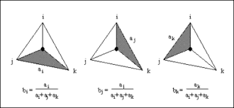
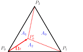
For many calculations, it is convenient to use barycentric coordinates to represent points in a triangle:
$$
\begin{aligned}
& \boldsymbol{x}=\lambda_1 \boldsymbol{v}_1+\lambda_2 \boldsymbol{v}_2+\lambda_3 \boldsymbol{v}_3 \quad \text { where } \
& 0 \leq \lambda_1, \lambda_2, \lambda_3 \text { and } \lambda_1+\lambda_2+\lambda_3=1,
\end{aligned}
$$
and $v_1, v_2, v_3$ are the vertices of the triangle. Note that the triangle $T$ with these vertices is the set of all convex combinations of $\boldsymbol{v}_1, \boldsymbol{v}_2, \boldsymbol{v}_3$; we write $T=\operatorname{co}\left{\boldsymbol{v}_1, \boldsymbol{v}_2, \boldsymbol{v}_3\right}$. Furthermore, each point in $T$ can be represented uniquely in the form of (4.3.1). The barycentric coordinates for a given point $\boldsymbol{x} \in T$ are written as $\lambda_1(\boldsymbol{x}), \lambda_2(\boldsymbol{x}), \lambda_3(\boldsymbol{x})$. Note that the vector of barycentric coordinates $\boldsymbol{\lambda}(\boldsymbol{x})$ is an affine function of $\boldsymbol{x}$ : $\boldsymbol{\lambda}(\boldsymbol{x})=A \boldsymbol{x}+\boldsymbol{b}$ for some matrix $A$ and vector $\boldsymbol{b}$.
Given a function $f: T \rightarrow \mathbb{R}$ we have the linear interpolant given by
$$
p(\boldsymbol{x})=f\left(\boldsymbol{v}_1\right) \lambda_1(\boldsymbol{x})+f\left(\boldsymbol{v}_2\right) \lambda_2(\boldsymbol{x})+f\left(\boldsymbol{v}_3\right) \lambda_3(\boldsymbol{x}) .
$$
Computing the barycentric coordinates can be done using some linear algebra: since $\boldsymbol{x}=\left[\boldsymbol{v}_1\left|\boldsymbol{v}_2\right| \boldsymbol{v}_3\right] \boldsymbol{\lambda}$ and $1=[1|1| 1] \boldsymbol{\lambda}$ we can combine them into
$$
\begin{aligned}
{\left[\begin{array}{c}
1 \
x
\end{array}\right] } & =\left[\begin{array}{ccc}
1 & 1 & 1 \
v_1 & v_2 & v_3
\end{array}\right] \lambda, \
\lambda & =\left[\begin{array}{ccc}
1 & 1 & 1 \
\boldsymbol{v}_1 & v_2 & v_3
\end{array}\right]^{-1}\left[\begin{array}{l}
1 \
\boldsymbol{x}
\end{array}\right] .
\end{aligned}
$$
数值分析代考
数学代写|数值分析代写numerical analysis代考|Higher Order Splines in One Variable
根据分段线性揷值的最小化原则 (4.2.1) 和三次样条的 (4.2.6),一个变量中的三次样条自然泛化。我们可 以要求找到
(4.2.10)min $s \int x_0^{x_n} s^{\prime \prime \prime}(x)^2 d x \quad$ 受制于 $s\left(x_i\right)=y_i, \quad i=0,1,2, \ldots, n$.
最小化器 $s(4.2 .10)$ 的 (4.2.10) 是具有连续四阶导数(不仅仅是三阶导数)的分段五次(五阶)多顶式。 将这些条件与揷值特性结合起来给出 $6 n-4$ 方程式 $6 n$ 的末知系数
$s(x)=a_i x^5+b_i x^4+c_i x^3+d_i x^2+e_i x+f_i$ 为了 $x_i \leq x \leq x_{i+1}$. 施加的四个额外条件给出了 不同类型的五次样条。自然五次样条具有以下特性 $s^{\prime}(x)=s^{\prime \prime}(x)=0$ 在 $x=x_0, x_n$; 钳位五次样条具 有以下属性 $s^{\prime}\left(x_0\right)=y_0^{\prime}, s^{\prime \prime}\left(x_0\right)=y_0^{\prime \prime}, s^{\prime}\left(x_n\right)=y_n^{\prime}$ ,和 $s^{\prime \prime}\left(x_n\right)=y_n^{\prime \prime}$ 都是指定的。在给定揷值 数据的情况下计算这些五次样条之一涉及求解五对角线 (5 对角线) 对称正定线性系统。
五次样条的优点是平滑度稍好,揷值振荡较少。它们的缺点是实施起来计算成本更高。 练习。
(1) 使用非结三次样条揷值 $f(x)=e^{-x} /(1+x)$ 超过 $[0,1]$ 使用 $n+1$ 等距揷值点
$n=5,10,20,40,100$. 估计之间的最大误差 $f$ 样条揷值使用 1001 个等距分布的点 $[0,1]$. 绘制最大误差 $n$. 估计指数 $\alpha$ 其中最大误差是渐近的 $C h^\alpha$. 这是否证实了理论误差估计 $\mathcal{O}\left(h^4\right)$ ?
(2) 计算非结样条揷值的勒贝格常数 $\max 0 \leq x \leq 1 \sum k=0^n\left|\ell_k(x)\right|$ 在哪里 $\ell_k$ 是非节点样条函数揷 值 $\ell_k\left(x_j\right)=1$ 如果 $j=k$ 如果为零 $j \neq k$. 使用等距揷值点 $x_j=j / n$ 为了 $j=0,1,2, \ldots, n$. 这样做是 为了 $n=5,10,20,40,100$.
(3) 要查看扰动的指数衰减,计算数据的非结样条揷值 $y_j=0$ 为了 $0 \leq j \leq N$ 除了那个 $y_{N / 2}=1$ 假设 $N$ 甚至; 还设置 $x_j=j, j=0,1,2, \ldots, N$. 这样做是为了 $N=100$. 估计样条揷值的指数衰减率 $s\left(x_j\right)$ 作 为 $|j-N / 2|$ 增加。重复这个 $x_j=j / N$.
数学代写|数值分析代写numerical analysis代考|Interpolation over Triangles
在一维空间中,基本形状通常非常简单:间隔。在二维中,有更多的选择,在三维中,基本形状的集合更 大。
在二维中,我们关注三角形。多边形可以分解成三角形。具有弯曲边界的域可以通过非重叒三角形的并集 来近似。联合中的三角形应该是“不重曡的”,至少在联合中不同三角形的交点是顶点或边的意义上。在三 个维度中,我们专注于四面体,以及四个和更高维度的单纯形,在这些维度中应用类似的方法和行为。
对于许多计算,使用重心坐标来表示三角形中的点会很方便:
$\boldsymbol{x}=\lambda_1 \boldsymbol{v}_1+\lambda_2 \boldsymbol{v}_2+\lambda_3 \boldsymbol{v}_3 \quad$ where $\quad 0 \leq \lambda_1, \lambda_2, \lambda_3$ and $\lambda_1+\lambda_2+\lambda_3=1$
和 $v_1, v_2, v_3$ 是三角形的顶点。注意三角形 $T$ 这些顶点是所有凸组合的集合 $\boldsymbol{v}_1, \boldsymbol{v}_2, \boldsymbol{v}_3$; 我们写 可以用 (4.3.1) 的形式唯一表示。给定点的重心坐标 $\boldsymbol{x} \in T$ 被写成 $\lambda_1(\boldsymbol{x}), \lambda_2(\boldsymbol{x}), \lambda_3(\boldsymbol{x})$. 请注意,重 心坐标的矢量 $\boldsymbol{\lambda}(\boldsymbol{x})$ 是仿射函数 $\boldsymbol{x}: \boldsymbol{\lambda}(\boldsymbol{x})=A \boldsymbol{x}+\boldsymbol{b}$ 对于一些矩阵 $A$ 和矢量 $\boldsymbol{b}$.
给定一个函数 $f: T \rightarrow \mathbb{R}$ 我们有线性揷值
$$
p(\boldsymbol{x})=f\left(\boldsymbol{v}_1\right) \lambda_1(\boldsymbol{x})+f\left(\boldsymbol{v}_2\right) \lambda_2(\boldsymbol{x})+f\left(\boldsymbol{v}_3\right) \lambda_3(\boldsymbol{x}) .
$$
计算重心坐标可以使用一些线性代数来完成: 因为 $\boldsymbol{x}=\left[\boldsymbol{v}_1\left|\boldsymbol{v}_2\right| \boldsymbol{v}_3\right] \boldsymbol{\lambda}$ 和 $1=[1|1| 1] \boldsymbol{\lambda}$ 我们可以将它们组合成

统计代写请认准statistics-lab™. statistics-lab™为您的留学生涯保驾护航。
金融工程代写
金融工程是使用数学技术来解决金融问题。金融工程使用计算机科学、统计学、经济学和应用数学领域的工具和知识来解决当前的金融问题,以及设计新的和创新的金融产品。
非参数统计代写
非参数统计指的是一种统计方法,其中不假设数据来自于由少数参数决定的规定模型;这种模型的例子包括正态分布模型和线性回归模型。
广义线性模型代考
广义线性模型(GLM)归属统计学领域,是一种应用灵活的线性回归模型。该模型允许因变量的偏差分布有除了正态分布之外的其它分布。
术语 广义线性模型(GLM)通常是指给定连续和/或分类预测因素的连续响应变量的常规线性回归模型。它包括多元线性回归,以及方差分析和方差分析(仅含固定效应)。
有限元方法代写
有限元方法(FEM)是一种流行的方法,用于数值解决工程和数学建模中出现的微分方程。典型的问题领域包括结构分析、传热、流体流动、质量运输和电磁势等传统领域。
有限元是一种通用的数值方法,用于解决两个或三个空间变量的偏微分方程(即一些边界值问题)。为了解决一个问题,有限元将一个大系统细分为更小、更简单的部分,称为有限元。这是通过在空间维度上的特定空间离散化来实现的,它是通过构建对象的网格来实现的:用于求解的数值域,它有有限数量的点。边界值问题的有限元方法表述最终导致一个代数方程组。该方法在域上对未知函数进行逼近。[1] 然后将模拟这些有限元的简单方程组合成一个更大的方程系统,以模拟整个问题。然后,有限元通过变化微积分使相关的误差函数最小化来逼近一个解决方案。
tatistics-lab作为专业的留学生服务机构,多年来已为美国、英国、加拿大、澳洲等留学热门地的学生提供专业的学术服务,包括但不限于Essay代写,Assignment代写,Dissertation代写,Report代写,小组作业代写,Proposal代写,Paper代写,Presentation代写,计算机作业代写,论文修改和润色,网课代做,exam代考等等。写作范围涵盖高中,本科,研究生等海外留学全阶段,辐射金融,经济学,会计学,审计学,管理学等全球99%专业科目。写作团队既有专业英语母语作者,也有海外名校硕博留学生,每位写作老师都拥有过硬的语言能力,专业的学科背景和学术写作经验。我们承诺100%原创,100%专业,100%准时,100%满意。
随机分析代写
随机微积分是数学的一个分支,对随机过程进行操作。它允许为随机过程的积分定义一个关于随机过程的一致的积分理论。这个领域是由日本数学家伊藤清在第二次世界大战期间创建并开始的。
时间序列分析代写
随机过程,是依赖于参数的一组随机变量的全体,参数通常是时间。 随机变量是随机现象的数量表现,其时间序列是一组按照时间发生先后顺序进行排列的数据点序列。通常一组时间序列的时间间隔为一恒定值(如1秒,5分钟,12小时,7天,1年),因此时间序列可以作为离散时间数据进行分析处理。研究时间序列数据的意义在于现实中,往往需要研究某个事物其随时间发展变化的规律。这就需要通过研究该事物过去发展的历史记录,以得到其自身发展的规律。
回归分析代写
多元回归分析渐进(Multiple Regression Analysis Asymptotics)属于计量经济学领域,主要是一种数学上的统计分析方法,可以分析复杂情况下各影响因素的数学关系,在自然科学、社会和经济学等多个领域内应用广泛。
MATLAB代写
MATLAB 是一种用于技术计算的高性能语言。它将计算、可视化和编程集成在一个易于使用的环境中,其中问题和解决方案以熟悉的数学符号表示。典型用途包括:数学和计算算法开发建模、仿真和原型制作数据分析、探索和可视化科学和工程图形应用程序开发,包括图形用户界面构建MATLAB 是一个交互式系统,其基本数据元素是一个不需要维度的数组。这使您可以解决许多技术计算问题,尤其是那些具有矩阵和向量公式的问题,而只需用 C 或 Fortran 等标量非交互式语言编写程序所需的时间的一小部分。MATLAB 名称代表矩阵实验室。MATLAB 最初的编写目的是提供对由 LINPACK 和 EISPACK 项目开发的矩阵软件的轻松访问,这两个项目共同代表了矩阵计算软件的最新技术。MATLAB 经过多年的发展,得到了许多用户的投入。在大学环境中,它是数学、工程和科学入门和高级课程的标准教学工具。在工业领域,MATLAB 是高效研究、开发和分析的首选工具。MATLAB 具有一系列称为工具箱的特定于应用程序的解决方案。对于大多数 MATLAB 用户来说非常重要,工具箱允许您学习和应用专业技术。工具箱是 MATLAB 函数(M 文件)的综合集合,可扩展 MATLAB 环境以解决特定类别的问题。可用工具箱的领域包括信号处理、控制系统、神经网络、模糊逻辑、小波、仿真等。