如果你也在 怎样代写常微分方程ordinary differential equation这个学科遇到相关的难题,请随时右上角联系我们的24/7代写客服。
常微分方程是为一个或多个独立变量的函数及其导数定义的方程。y’=x+1是一个常微分方程的例子。
statistics-lab™ 为您的留学生涯保驾护航 在代写常微分方程ordinary differential equation方面已经树立了自己的口碑, 保证靠谱, 高质且原创的统计Statistics代写服务。我们的专家在代写常微分方程ordinary differential equation代写方面经验极为丰富,各种代写常微分方程ordinary differential equation相关的作业也就用不着说。
我们提供的常微分方程ordinary differential equation及其相关学科的代写,服务范围广, 其中包括但不限于:
- Statistical Inference 统计推断
- Statistical Computing 统计计算
- Advanced Probability Theory 高等概率论
- Advanced Mathematical Statistics 高等数理统计学
- (Generalized) Linear Models 广义线性模型
- Statistical Machine Learning 统计机器学习
- Longitudinal Data Analysis 纵向数据分析
- Foundations of Data Science 数据科学基础
数学代写|常微分方程代写ordinary differential equation代考|Existence and Uniqueness
Let $J \subseteq \mathbb{R}, U \subseteq \mathbb{R}^n$, and $\Lambda \subseteq \mathbb{R}^k$ be open subsets, and suppose that $f: J \times U \times \Lambda \rightarrow \mathbb{R}^n$ is a smooth function. Here the term “smooth” means that the function $f$ is continuously differentiable. An ordinary differential equation (ODE) is an equation of the form
$$
\dot{x}=f(t, x, \lambda)
$$
where the dot denotes differentiation with respect to the independent variable $t$ (usually a measure of time), the dependent variable $x$ is a vector of state variables, and $\lambda$ is a vector of parameters. As convenient terminology, especially when we are concerned with the components of a vector differential equation, we will say that equation (1.1) is a system of differential equations. Also, if we are interested in changes with respect to parameters, then the differential equation is called a family of differential equations.
Example 1.1. The forced van der Pol oscillator
$$
\begin{aligned}
& \dot{x}_1=x_2, \
& \dot{x}_2=b\left(1-x_1^2\right) x_2-\omega^2 x_1+a \cos \Omega t
\end{aligned}
$$
is a differential equation with $J=\mathbb{R}, x=\left(x_1, x_2\right) \in U=\mathbb{R}^2$,
$$
\Lambda=\left{(a, b, \omega, \Omega):(a, b) \in \mathbb{R}^2, \omega>0, \Omega>0\right},
$$
and $f: \mathbb{R} \times \mathbb{R}^2 \times \Lambda \rightarrow \mathbb{R}^2$ defined in components by
$$
\left(t, x_1, x_2, a, b, \omega, \Omega\right) \mapsto\left(x_2, b\left(1-x_1^2\right) x_2-\omega^2 x_1+a \cos \Omega t\right) .
$$
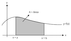
If $\lambda \in \Lambda$ is fixed, then a solution of the differential equation (1.1) is a function $\phi: J_0 \rightarrow U$ given by $t \mapsto \phi(t)$, where $J_0$ is an open subset of $J$, such that
$$
\frac{d \phi}{d t}(t)=f(t, \phi(t), \lambda)
$$
for all $t \in J_0$.
In this context, the words “trajectory,” “phase curve,” and “integral curve” are also used to refer to solutions of the differential equation (1.1). However, it is useful to have a term that refers to the image of the solution in $\mathbb{R}^n$. Thus, we define the orbit of the solution $\phi$ to be the set ${\phi(t) \in U$ : $\left.t \in J_0\right}$
数学代写|常微分方程代写ordinary differential equation代考|Types of Differential Equations
Differential equations may be classified in several different ways. In this section we note that the independent variable may be implicit or explicit, and that higher order derivatives may appear.
An autonomous differential equation is given by
$$
\dot{x}=f(x, \lambda), \quad x \in \mathbb{R}^n, \quad \lambda \in \mathbb{R}^k ;
$$
that is, the function $f$ does not depend explicitly on the independent variable. If the function $f$ does depend explicitly on $t$, then the corresponding differential equation is called nonautonomous.
In physical applications, we often encounter equations containing second, third, or higher order derivatives with respect to the independent variable. These are called second order differential equations, third order differential equations, and so on, where the the order of the equation refers to the order of the highest order derivative with respect to the independent variable that appears explicitly. In this hierarchy, a differential equation is called a first order differential equation.
Recall that Newton’s second law-the rate of change of the linear momentum acting on a body is equal to the sum of the forces acting on the body -involves the second derivative of the position of the body with respect to time. Thus, in many physical applications the most common differential equations used as mathematical models are second order differential equations. For example, the natural physical derivation of van der Pol’s equation leads to a second order differential equation of the form
$$
\ddot{u}+b\left(u^2-1\right) \dot{u}+\omega^2 u=a \cos \Omega t .
$$
An essential fact is that every differential equation is equivalent to a first order system. To illustrate, let us consider the conversion of van der Pol’s equation to a first order system. For this, we simply define a new variable $v:=\dot{u}$ so that we obtain the following system:
$$
\begin{aligned}
\dot{u} & =v \
\dot{v} & =-\omega^2 u+b\left(1-u^2\right) v+a \cos \Omega t .
\end{aligned}
$$
常微分方程代写
数学代写|常微分方程代写ordinary differential equation代考|Existence and Uniqueness
让 $J \subseteq \mathbb{R}, U \subseteq \mathbb{R}^n$ ,和 $\Lambda \subseteq \mathbb{R}^k$ 是开子集,并假设 $f: J \times U \times \Lambda \rightarrow \mathbb{R}^n$ 是平滑函数。这里术语 “平 滑”意味着函数 $f$ 是连续可微的。常微分方程 (ODE) 是以下形式的方程
$$
\dot{x}=f(t, x, \lambda)
$$
其中点表示相对于自变量的微分 $t$ (通常是时间的度量),因变量 $x$ 是状态变量的向量,并且 $\lambda$ 是一个参数 向量。作为方便的术语,特别是当我们关注向量微分方程的分量时,我们会说方程 (1.1) 是一个微分方程 组。此外,如果我们对参数的变化感兴趣,则微分方程称为微分方程族。
示例 1.1。强制范德波尔振荡器
$$
\dot{x}_1=x_2, \quad \dot{x}_2=b\left(1-x_1^2\right) x_2-\omega^2 x_1+a \cos \Omega t
$$
是一个微分方程 $J=\mathbb{R}, x=\left(x_1, x_2\right) \in U=\mathbb{R}^2$ ,
ILambda $=\backslash$ eft $\left{\left(a, b\right.\right.$, Iomega, \Omega):(a, b) \in $\backslash m a t h b b{R}^{\wedge} 2$, lomega $>0$, \Omega $>0$ \right } } \text { , }
和 $f: \mathbb{R} \times \mathbb{R}^2 \times \Lambda \rightarrow \mathbb{R}^2$ 在组件中定义
$$
\left(t, x_1, x_2, a, b, \omega, \Omega\right) \mapsto\left(x_2, b\left(1-x_1^2\right) x_2-\omega^2 x_1+a \cos \Omega t\right) .
$$
如果 $\lambda \in \Lambda$ 是固定的,则微分方程 (1.1) 的解是一个函数 $\phi: J_0 \rightarrow U$ 由 $t \mapsto \phi(t)$ ,在哪里 $J_0$ 是一个 开子集 $J$, 这样
$$
\frac{d \phi}{d t}(t)=f(t, \phi(t), \lambda)
$$
对所有人 $t \in J_0$.
在这种情况下,”轨迹”、“相位曲线”和”积分曲线”等词也用于指代微分方程 (1.1) 的解。但是,使用一个术 语来引用解决方案的图像是很有用的 $\mathbb{R}^n$. 因此,我们定义解的轨道 $\phi$ 成为集合
数学代写|常微分方程代写ordinary differential equation代考|Types of Differential Equations
微分方程可以用几种不同的方式分类。在本节中,我们注意到自变量可能是隐式的或显式的,并且可能出 现高阶导数。
自主微分方程由下式给出
$$
\dot{x}=f(x, \lambda), \quad x \in \mathbb{R}^n, \quad \lambda \in \mathbb{R}^k ;
$$
即函数 $f$ 不明确依赖于自变量。如果函数 $f$ 确实明确地依赖于 $t$ ,则相应的微分方程称为非自治微分方程。
在物理应用中,我们经常遇到包含关于自变量的二阶、三阶或更高阶导数的方程。这些被称为二阶微分方 程、三阶微分方程等,其中方程的阶数是指相对于显式出现的自变量的最高阶导数的阶数。在这个层次 中,微分方程称为一阶微分方程。
回想一下牛顿第二定律一一作用在物体上的线性动量的变化率等于作用在物体上的力的总和一一涉及物体 位置相对于时间的二阶导数。因此,在许多物理应用中,用作数学模型的最常见的微分方程是二阶微分方 程。例如,van der Pol 方程的自然物理推导导致二阶微分方程的形式
$$
\ddot{u}+b\left(u^2-1\right) \dot{u}+\omega^2 u=a \cos \Omega t .
$$
一个重要的事实是每个微分方程都等价于一阶系统。为了说明,让我们考虑将 van der Pol 方程转换为一 阶系统。为此,我们只需定义一个新变量 $v:=\dot{u}$ 从而得到如下系统:
$$
\dot{u}=v \dot{v} \quad=-\omega^2 u+b\left(1-u^2\right) v+a \cos \Omega t .
$$

统计代写请认准statistics-lab™. statistics-lab™为您的留学生涯保驾护航。
金融工程代写
金融工程是使用数学技术来解决金融问题。金融工程使用计算机科学、统计学、经济学和应用数学领域的工具和知识来解决当前的金融问题,以及设计新的和创新的金融产品。
非参数统计代写
非参数统计指的是一种统计方法,其中不假设数据来自于由少数参数决定的规定模型;这种模型的例子包括正态分布模型和线性回归模型。
广义线性模型代考
广义线性模型(GLM)归属统计学领域,是一种应用灵活的线性回归模型。该模型允许因变量的偏差分布有除了正态分布之外的其它分布。
术语 广义线性模型(GLM)通常是指给定连续和/或分类预测因素的连续响应变量的常规线性回归模型。它包括多元线性回归,以及方差分析和方差分析(仅含固定效应)。
有限元方法代写
有限元方法(FEM)是一种流行的方法,用于数值解决工程和数学建模中出现的微分方程。典型的问题领域包括结构分析、传热、流体流动、质量运输和电磁势等传统领域。
有限元是一种通用的数值方法,用于解决两个或三个空间变量的偏微分方程(即一些边界值问题)。为了解决一个问题,有限元将一个大系统细分为更小、更简单的部分,称为有限元。这是通过在空间维度上的特定空间离散化来实现的,它是通过构建对象的网格来实现的:用于求解的数值域,它有有限数量的点。边界值问题的有限元方法表述最终导致一个代数方程组。该方法在域上对未知函数进行逼近。[1] 然后将模拟这些有限元的简单方程组合成一个更大的方程系统,以模拟整个问题。然后,有限元通过变化微积分使相关的误差函数最小化来逼近一个解决方案。
tatistics-lab作为专业的留学生服务机构,多年来已为美国、英国、加拿大、澳洲等留学热门地的学生提供专业的学术服务,包括但不限于Essay代写,Assignment代写,Dissertation代写,Report代写,小组作业代写,Proposal代写,Paper代写,Presentation代写,计算机作业代写,论文修改和润色,网课代做,exam代考等等。写作范围涵盖高中,本科,研究生等海外留学全阶段,辐射金融,经济学,会计学,审计学,管理学等全球99%专业科目。写作团队既有专业英语母语作者,也有海外名校硕博留学生,每位写作老师都拥有过硬的语言能力,专业的学科背景和学术写作经验。我们承诺100%原创,100%专业,100%准时,100%满意。
随机分析代写
随机微积分是数学的一个分支,对随机过程进行操作。它允许为随机过程的积分定义一个关于随机过程的一致的积分理论。这个领域是由日本数学家伊藤清在第二次世界大战期间创建并开始的。
时间序列分析代写
随机过程,是依赖于参数的一组随机变量的全体,参数通常是时间。 随机变量是随机现象的数量表现,其时间序列是一组按照时间发生先后顺序进行排列的数据点序列。通常一组时间序列的时间间隔为一恒定值(如1秒,5分钟,12小时,7天,1年),因此时间序列可以作为离散时间数据进行分析处理。研究时间序列数据的意义在于现实中,往往需要研究某个事物其随时间发展变化的规律。这就需要通过研究该事物过去发展的历史记录,以得到其自身发展的规律。
回归分析代写
多元回归分析渐进(Multiple Regression Analysis Asymptotics)属于计量经济学领域,主要是一种数学上的统计分析方法,可以分析复杂情况下各影响因素的数学关系,在自然科学、社会和经济学等多个领域内应用广泛。
MATLAB代写
MATLAB 是一种用于技术计算的高性能语言。它将计算、可视化和编程集成在一个易于使用的环境中,其中问题和解决方案以熟悉的数学符号表示。典型用途包括:数学和计算算法开发建模、仿真和原型制作数据分析、探索和可视化科学和工程图形应用程序开发,包括图形用户界面构建MATLAB 是一个交互式系统,其基本数据元素是一个不需要维度的数组。这使您可以解决许多技术计算问题,尤其是那些具有矩阵和向量公式的问题,而只需用 C 或 Fortran 等标量非交互式语言编写程序所需的时间的一小部分。MATLAB 名称代表矩阵实验室。MATLAB 最初的编写目的是提供对由 LINPACK 和 EISPACK 项目开发的矩阵软件的轻松访问,这两个项目共同代表了矩阵计算软件的最新技术。MATLAB 经过多年的发展,得到了许多用户的投入。在大学环境中,它是数学、工程和科学入门和高级课程的标准教学工具。在工业领域,MATLAB 是高效研究、开发和分析的首选工具。MATLAB 具有一系列称为工具箱的特定于应用程序的解决方案。对于大多数 MATLAB 用户来说非常重要,工具箱允许您学习和应用专业技术。工具箱是 MATLAB 函数(M 文件)的综合集合,可扩展 MATLAB 环境以解决特定类别的问题。可用工具箱的领域包括信号处理、控制系统、神经网络、模糊逻辑、小波、仿真等。