标签: ACTL90003

金融代写|利率建模代写Interest Rate Modeling代考|MATH5985

如果你也在 怎样代写利率建模Interest Rate Modeling这个学科遇到相关的难题,请随时右上角联系我们的24/7代写客服。

利率模型是指一种对利率的运动和演变进行建模的数学方法。它是一种基于市场风险的单因素短利率模型。瓦西克利率模型常用于经济学中,以确定利率在未来的移动方向。

statistics-lab™ 为您的留学生涯保驾护航 在代写利率建模Interest Rate Modeling方面已经树立了自己的口碑, 保证靠谱, 高质且原创的统计Statistics代写服务。我们的专家在代写利率建模Interest Rate Modeling代写方面经验极为丰富,各种代写利率建模Interest Rate Modeling相关的作业也就用不着说。

我们提供的利率建模Interest Rate Modeling及其相关学科的代写,服务范围广, 其中包括但不限于:

  • Statistical Inference 统计推断
  • Statistical Computing 统计计算
  • Advanced Probability Theory 高等概率论
  • Advanced Mathematical Statistics 高等数理统计学
  • (Generalized) Linear Models 广义线性模型
  • Statistical Machine Learning 统计机器学习
  • Longitudinal Data Analysis 纵向数据分析
  • Foundations of Data Science 数据科学基础
金融代写|利率建模代写Interest Rate Modeling代考|MATH5985

金融代写|利率建模代写Interest Rate Modeling代考| A Binomial Tree for the Ho–Lee Model

The IIo-Lee model was first presented with a binomial tree. For a Gaussian short-rate model with mean and variance of change over $(t, t+\Delta t)$ given by
$$
\begin{aligned}
E^{\mathbb{Q}}\left[\Delta r_t\right] &=\theta_t \Delta t \
\operatorname{VaR}\left(\Delta r_t\right) &=\sigma^2 \Delta t
\end{aligned}
$$
we consider a rather natural binomial tree approximation as illustrated in Figure 5.1, where, without loss of generality, the branching probabilities are uniformly one half.
For notational efficiency, we let
$$
r_{i, n}=r_{0,0}+\Delta t \sum_{k=1}^{n-1} \theta_k+(2 i-n) \sigma \sqrt{\Delta t}, \quad i=0,1, \ldots, n
$$

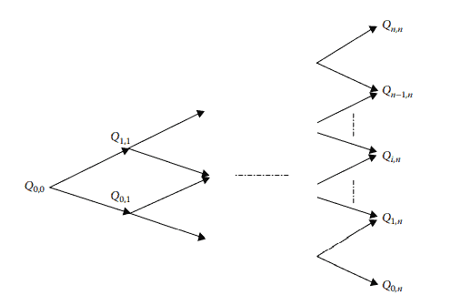
Then we have a multi-period tree as shown in Figure 5.2.
Before being applied to derivatives pricing, such a tree must first be calibrated to the current term structure of the interest rate. For the Ho-Lee model, we need to determine the drift, $\theta_t$, by reproducing the prices of zero-coupon bonds of all maturities. This task can be efficiently achieved with the help of the so-called Arrow-Debreu prices.

金融代写|利率建模代写Interest Rate Modeling代考|Arrow–Debreu Prices

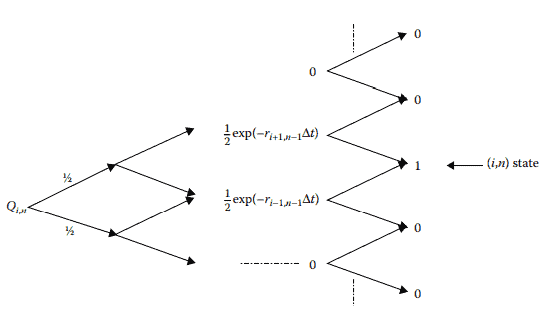
An Arrow-Debreu (1954) security is a canonical asset that has a cash flow of $\$ 1$ if a particular state (of interest rate) is realized, or nothing otherwise. The pattern of payment is shown in Figure $5.3$, where we let $Q_{i, j}$ denote the price of the security at time 0 that would pay $\$ 1$ at time $j$ if the state $i$ is realized, or nothing if otherwise.

Note that a zero-coupon bond can be regarded as a portfolio of ArrowDebreu securities. By linearity, the price of the zero-coupon bond maturing in time $j$ is equal to
$$
P(0, j)=\sum_{i=0}^j Q_{i, j} .
$$
Given an interest-rate tree as in Figure 5.2, we can construct the ArrowDebreu tree through a forward induction process. We begin with
$$
Q_{0,0}=1 .
$$
The calculations of $Q_{1,1}$ and $Q_{0,1}$ are done by “expectation pricing” using the trees in Figure $5.4$, where $r_{0,0}$ is the discount rate at node $(0,0)$. Intuitively, the prices of the two Arrow-Debreu securities are given by
$$
Q_{1,1}=Q_{0,1}=\frac{1}{2} \mathrm{e}^{-r_{0,0} \Delta t}
$$

金融代写|利率建模代写Interest Rate Modeling代考|MATH5985

利率建模代考

金融代写|利率建模代写利率建模代考| Ho-Lee模型的二叉树


IIo-Lee模型首先用二叉树表示。对于均值和方差大于$(t, t+\Delta t)$的高斯短期速率模型(
$$
\begin{aligned}
E^{\mathbb{Q}}\left[\Delta r_t\right] &=\theta_t \Delta t \
\operatorname{VaR}\left(\Delta r_t\right) &=\sigma^2 \Delta t
\end{aligned}
$$
),我们考虑一种相当自然的二叉树近似,如图5.1所示,在不丧失一般性的情况下,分支概率一致为1 / 2。
为了符号效率,我们让
$$
r_{i, n}=r_{0,0}+\Delta t \sum_{k=1}^{n-1} \theta_k+(2 i-n) \sigma \sqrt{\Delta t}, \quad i=0,1, \ldots, n
$$


然后我们就有了一个如图5.2所示的多周期树。在应用于衍生品定价之前,这种树必须首先根据当前利率的期限结构进行校准。对于Ho-Lee模型,我们需要通过再现所有期限的零息债券的价格来确定漂移$\theta_t$。在所谓的阿罗-德布鲁价格的帮助下,这一任务可以有效地完成

金融代写|利率建模代写Interest Rate Modeling代考| 阿罗-德布鲁·普莱斯


a Arrow-Debreu(1954)证券是一种典型资产,如果实现了特定的(利率)状态,或者其他什么都没有,那么它的现金流为$\$ 1$。支付模式如图$5.3$所示,其中我们让$Q_{i, j}$表示时间0时的证券价格,如果状态$i$实现,则在时间$j$时支付$\$ 1$,否则则不支付


请注意,零息债券可以被视为ArrowDebreu证券的投资组合。通过线性关系,及时$j$到期的零息债券价格等于
$$
P(0, j)=\sum_{i=0}^j Q_{i, j} .
$$
给定如图5.2所示的利率树,我们可以通过正向归纳过程构建ArrowDebreu树。我们从
$$
Q_{0,0}=1 .
$$
开始,$Q_{1,1}$和$Q_{0,1}$的计算通过使用图$5.4$中的树的“期望定价”来完成,其中$r_{0,0}$是节点$(0,0)$上的贴现率。直观地看,这两种Arrow-Debreu证券的价格由
$$
Q_{1,1}=Q_{0,1}=\frac{1}{2} \mathrm{e}^{-r_{0,0} \Delta t}
$$ 给出

金融代写|利率建模代写Interest Rate Modeling代考 请认准statistics-lab™

统计代写请认准statistics-lab™. statistics-lab™为您的留学生涯保驾护航。

金融工程代写

金融工程是使用数学技术来解决金融问题。金融工程使用计算机科学、统计学、经济学和应用数学领域的工具和知识来解决当前的金融问题,以及设计新的和创新的金融产品。

非参数统计代写

非参数统计指的是一种统计方法,其中不假设数据来自于由少数参数决定的规定模型;这种模型的例子包括正态分布模型和线性回归模型。

广义线性模型代考

广义线性模型(GLM)归属统计学领域,是一种应用灵活的线性回归模型。该模型允许因变量的偏差分布有除了正态分布之外的其它分布。

术语 广义线性模型(GLM)通常是指给定连续和/或分类预测因素的连续响应变量的常规线性回归模型。它包括多元线性回归,以及方差分析和方差分析(仅含固定效应)。

有限元方法代写

有限元方法(FEM)是一种流行的方法,用于数值解决工程和数学建模中出现的微分方程。典型的问题领域包括结构分析、传热、流体流动、质量运输和电磁势等传统领域。

有限元是一种通用的数值方法,用于解决两个或三个空间变量的偏微分方程(即一些边界值问题)。为了解决一个问题,有限元将一个大系统细分为更小、更简单的部分,称为有限元。这是通过在空间维度上的特定空间离散化来实现的,它是通过构建对象的网格来实现的:用于求解的数值域,它有有限数量的点。边界值问题的有限元方法表述最终导致一个代数方程组。该方法在域上对未知函数进行逼近。[1] 然后将模拟这些有限元的简单方程组合成一个更大的方程系统,以模拟整个问题。然后,有限元通过变化微积分使相关的误差函数最小化来逼近一个解决方案。

tatistics-lab作为专业的留学生服务机构,多年来已为美国、英国、加拿大、澳洲等留学热门地的学生提供专业的学术服务,包括但不限于Essay代写,Assignment代写,Dissertation代写,Report代写,小组作业代写,Proposal代写,Paper代写,Presentation代写,计算机作业代写,论文修改和润色,网课代做,exam代考等等。写作范围涵盖高中,本科,研究生等海外留学全阶段,辐射金融,经济学,会计学,审计学,管理学等全球99%专业科目。写作团队既有专业英语母语作者,也有海外名校硕博留学生,每位写作老师都拥有过硬的语言能力,专业的学科背景和学术写作经验。我们承诺100%原创,100%专业,100%准时,100%满意。

随机分析代写


随机微积分是数学的一个分支,对随机过程进行操作。它允许为随机过程的积分定义一个关于随机过程的一致的积分理论。这个领域是由日本数学家伊藤清在第二次世界大战期间创建并开始的。

时间序列分析代写

随机过程,是依赖于参数的一组随机变量的全体,参数通常是时间。 随机变量是随机现象的数量表现,其时间序列是一组按照时间发生先后顺序进行排列的数据点序列。通常一组时间序列的时间间隔为一恒定值(如1秒,5分钟,12小时,7天,1年),因此时间序列可以作为离散时间数据进行分析处理。研究时间序列数据的意义在于现实中,往往需要研究某个事物其随时间发展变化的规律。这就需要通过研究该事物过去发展的历史记录,以得到其自身发展的规律。

回归分析代写

多元回归分析渐进(Multiple Regression Analysis Asymptotics)属于计量经济学领域,主要是一种数学上的统计分析方法,可以分析复杂情况下各影响因素的数学关系,在自然科学、社会和经济学等多个领域内应用广泛。

MATLAB代写

MATLAB 是一种用于技术计算的高性能语言。它将计算、可视化和编程集成在一个易于使用的环境中,其中问题和解决方案以熟悉的数学符号表示。典型用途包括:数学和计算算法开发建模、仿真和原型制作数据分析、探索和可视化科学和工程图形应用程序开发,包括图形用户界面构建MATLAB 是一个交互式系统,其基本数据元素是一个不需要维度的数组。这使您可以解决许多技术计算问题,尤其是那些具有矩阵和向量公式的问题,而只需用 C 或 Fortran 等标量非交互式语言编写程序所需的时间的一小部分。MATLAB 名称代表矩阵实验室。MATLAB 最初的编写目的是提供对由 LINPACK 和 EISPACK 项目开发的矩阵软件的轻松访问,这两个项目共同代表了矩阵计算软件的最新技术。MATLAB 经过多年的发展,得到了许多用户的投入。在大学环境中,它是数学、工程和科学入门和高级课程的标准教学工具。在工业领域,MATLAB 是高效研究、开发和分析的首选工具。MATLAB 具有一系列称为工具箱的特定于应用程序的解决方案。对于大多数 MATLAB 用户来说非常重要,工具箱允许您学习应用专业技术。工具箱是 MATLAB 函数(M 文件)的综合集合,可扩展 MATLAB 环境以解决特定类别的问题。可用工具箱的领域包括信号处理、控制系统、神经网络、模糊逻辑、小波、仿真等。

R语言代写问卷设计与分析代写
PYTHON代写回归分析与线性模型代写
MATLAB代写方差分析与试验设计代写
STATA代写机器学习/统计学习代写
SPSS代写计量经济学代写
EVIEWS代写时间序列分析代写
EXCEL代写深度学习代写
SQL代写各种数据建模与可视化代写

金融代写|利率建模代写Interest Rate Modeling代考|ACTL40004

如果你也在 怎样代写利率建模Interest Rate Modeling这个学科遇到相关的难题,请随时右上角联系我们的24/7代写客服。

利率模型是指一种对利率的运动和演变进行建模的数学方法。它是一种基于市场风险的单因素短利率模型。瓦西克利率模型常用于经济学中,以确定利率在未来的移动方向。

statistics-lab™ 为您的留学生涯保驾护航 在代写利率建模Interest Rate Modeling方面已经树立了自己的口碑, 保证靠谱, 高质且原创的统计Statistics代写服务。我们的专家在代写利率建模Interest Rate Modeling代写方面经验极为丰富,各种代写利率建模Interest Rate Modeling相关的作业也就用不着说。

我们提供的利率建模Interest Rate Modeling及其相关学科的代写,服务范围广, 其中包括但不限于:

  • Statistical Inference 统计推断
  • Statistical Computing 统计计算
  • Advanced Probability Theory 高等概率论
  • Advanced Mathematical Statistics 高等数理统计学
  • (Generalized) Linear Models 广义线性模型
  • Statistical Machine Learning 统计机器学习
  • Longitudinal Data Analysis 纵向数据分析
  • Foundations of Data Science 数据科学基础
金融代写|利率建模代写Interest Rate Modeling代考|ACTL40004

金融代写|利率建模代写Interest Rate Modeling代考| GENERAL MARKOVIAN MODELS

Existing short-rate models are Markovian models. A no-arbitrage shortrate model should also be derived from the HJM framework. However, this can be quite difficult. In this section, we address the opposite question: under what kind of forward-rate volatility specifications should the resulting short-rate model be a Markovian random variable? Answering this question will help us to calibrate and implement a short-rate model more efficiently.
According to Equation 4.21, the short rate can be expressed as
$$
r_t=f(t, t)=f(0, t)+\int_0^t\left[-\boldsymbol{\sigma}^{\mathrm{T}}(s, t) \mathbf{\Sigma}(s, t) \mathrm{d} s+\boldsymbol{\sigma}^{\mathrm{T}}(s, t) \mathrm{d} \mathbf{W}_s\right]
$$

where $\mathbf{W}t$ is the $n$-dimensional Brownian motion under the risk-neutral measure, $\sigma(t, T)$ the forward-rate volatility, and $\boldsymbol{\Sigma}(t, T)$ the volatility of the $T$-maturity zero-coupon bond, given by $\boldsymbol{\Sigma}(t, T)=-\int_t^T \boldsymbol{\sigma}(t, u) \mathrm{d} u$. The stochastic differentiation of the short rate is $$ \begin{aligned} \mathrm{d} r_t=& {\left[f_t(0, t)+\int_0^t\left(-\frac{\partial}{\partial t}\left(\boldsymbol{\sigma}^{\mathrm{T}}(s, t) \boldsymbol{\Sigma}(s, t)\right) \mathrm{d} s+\frac{\partial \boldsymbol{\sigma}^{\mathrm{T}}(s, t)}{\partial t} \mathrm{~d} \mathbf{W}_s\right)\right] \mathrm{d} t } \ &+\boldsymbol{\sigma}^{\mathrm{T}}(t, t) \mathrm{d} \mathbf{W}_t \ =& {\left[f_t(t, T)\right]{T=t} \mathrm{~d} t+\boldsymbol{\sigma}^{\mathrm{T}}(t, t) \mathrm{d}t . } \end{aligned} $$ Based on Equation $5.17$ we can make the following judgment: for the shortrate model to be a Markovian process, we need the drift term, $\left[f_t(t, T)\right]{T=t}$, to be a function of a finite set of state variables that are jointly Markovian in their evolution.

To write the short rate as a function of several state variables, we introduce auxiliary functions
$$
b_i(t, T)=\sigma_i(t, T) \int_t^T \sigma_i(t, s) \mathrm{d} s, \quad i=1,2, \ldots, n .
$$

金融代写|利率建模代写Interest Rate Modeling代考|Monte Carlo Simulations for Options Pricing

Owing to the Markovian property of short-rate models, path simulations by Monte Carlo methods can be carried out efficiently, which is important for pricing exotic and path-dependent options. Take the pricing of the option on a zero-coupon for example. The value can be expressed as
$$
V_t=E_t^{\mathbb{Q}}\left[\mathrm{e}^{-\int_t^T r_s \mathrm{~d} s}(P(T, \tau)-K)^{+}\right], \quad t<T<\tau
$$
where $\mathbb{Q}$ stands for the risk-neutral measure, $r_t$ is given by Equation $5.20$, and the bond price is given by Equation 5.39. Both variables are expressed in terms of $\chi_i(t)$ and $\varphi_i(t), i=1, \ldots, n$, which evolve according to Equation 5.23. The corresponding simulation scheme for $\chi_i(t)$ and $\varphi_i(t)$ is
$$
\begin{aligned}
&\varphi_i(t+\Delta t)-\varphi_i(t)+\left(\sigma_i^2(t, t)-2 \kappa_i(t) \varphi_i(t)\right) \Delta t \
&\chi_i(t+\Delta t)=\chi_i(t)+\left(\varphi_i(t)-\kappa_i(t) \chi_i(t)\right) \mathrm{d} t+\sigma_i(t, t) \Delta W_i(t)
\end{aligned}
$$
which is simply the so-called Euler scheme. The bond option is priced by simulating many payoffs before taking an average.
In Inui and Kijima (1998), the following example is considered:
$$
\boldsymbol{\sigma}(t, T)=\left(\begin{array}{c}
c_1 r_t^\alpha \
c_2 r_t^\beta \mathrm{e}^{-\kappa(T-t)}
\end{array}\right)
$$
where $c_i, i=1,2, \alpha, \beta$, and $\kappa$ are non-negative constants. It can be verified that the components of the volatility vector satisfy
$$
\frac{\partial \sigma_1(t, T)}{\partial T}=0, \quad \frac{\partial \sigma_2(t, T)}{\partial T}=-\kappa \sigma_2(t, T) .
$$

金融代写|利率建模代写Interest Rate Modeling代考|ACTL40004

利率建模代考

金融代写|利率建模代写Interest Rate Modeling代考| 一般马尔可夫模型


现有的短期利率模型是马尔可夫模型。还应该从HJM框架推导出无套利的短期模型。然而,这是相当困难的。在本节中,我们将讨论相反的问题:在什么样的远期利率波动率规范下,所得到的短期利率模型应该是一个马尔可夫随机变量?回答这个问题将有助于我们更有效地校准和实施短期利率模型。根据公式4.21,短期汇率可表示为
$$
r_t=f(t, t)=f(0, t)+\int_0^t\left[-\boldsymbol{\sigma}^{\mathrm{T}}(s, t) \mathbf{\Sigma}(s, t) \mathrm{d} s+\boldsymbol{\sigma}^{\mathrm{T}}(s, t) \mathrm{d} \mathbf{W}_s\right]
$$

where $\mathbf{W}t$ 是 $n$风险中性测度下的-维布朗运动, $\sigma(t, T)$ 远期利率波动 $\boldsymbol{\Sigma}(t, T)$ 波动率 $T$到期零息债券,由 $\boldsymbol{\Sigma}(t, T)=-\int_t^T \boldsymbol{\sigma}(t, u) \mathrm{d} u$。短期汇率的随机微分是 $$ \begin{aligned} \mathrm{d} r_t=& {\left[f_t(0, t)+\int_0^t\left(-\frac{\partial}{\partial t}\left(\boldsymbol{\sigma}^{\mathrm{T}}(s, t) \boldsymbol{\Sigma}(s, t)\right) \mathrm{d} s+\frac{\partial \boldsymbol{\sigma}^{\mathrm{T}}(s, t)}{\partial t} \mathrm{~d} \mathbf{W}_s\right)\right] \mathrm{d} t } \ &+\boldsymbol{\sigma}^{\mathrm{T}}(t, t) \mathrm{d} \mathbf{W}_t \ =& {\left[f_t(t, T)\right]{T=t} \mathrm{~d} t+\boldsymbol{\sigma}^{\mathrm{T}}(t, t) \mathrm{d}t . } \end{aligned} $$ 基于方程 $5.17$ 我们可以做出以下判断:要使短期模型为马尔可夫过程,我们需要漂移项, $\left[f_t(t, T)\right]{T=t}$,是一组有限状态变量的函数,这些状态变量在演化过程中共同具有马尔可夫性 为了将短期汇率写成几个状态变量的函数,我们引入了辅助函数
$$
b_i(t, T)=\sigma_i(t, T) \int_t^T \sigma_i(t, s) \mathrm{d} s, \quad i=1,2, \ldots, n .
$$

金融代写|利率建模代写利率建模代考|期权定价的蒙特卡洛模拟


由于短期利率模型的马尔可夫性质,蒙特卡洛方法可以有效地进行路径模拟,这对奇异和路径相关期权的定价是重要的。以零息票的期权定价为例。取值可以表示为
$$
V_t=E_t^{\mathbb{Q}}\left[\mathrm{e}^{-\int_t^T r_s \mathrm{~d} s}(P(T, \tau)-K)^{+}\right], \quad t<T<\tau
$$
,其中$\mathbb{Q}$表示风险中性测度,$r_t$由式$5.20$给出,债券价格由式5.39给出。两个变量都用$\chi_i(t)$和$\varphi_i(t), i=1, \ldots, n$表示,根据公式5.23进行演化。$\chi_i(t)$和$\varphi_i(t)$对应的模拟方案是
$$
\begin{aligned}
&\varphi_i(t+\Delta t)-\varphi_i(t)+\left(\sigma_i^2(t, t)-2 \kappa_i(t) \varphi_i(t)\right) \Delta t \
&\chi_i(t+\Delta t)=\chi_i(t)+\left(\varphi_i(t)-\kappa_i(t) \chi_i(t)\right) \mathrm{d} t+\sigma_i(t, t) \Delta W_i(t)
\end{aligned}
$$
,这就是所谓的欧拉方案。债券期权的定价是通过在取平均值之前模拟许多支付进行的。在Inui和Kijima(1998)中,考虑以下例子:
$$
\boldsymbol{\sigma}(t, T)=\left(\begin{array}{c}
c_1 r_t^\alpha \
c_2 r_t^\beta \mathrm{e}^{-\kappa(T-t)}
\end{array}\right)
$$
其中$c_i, i=1,2, \alpha, \beta$和$\kappa$是非负常数。可以验证,波动率向量的分量满足
$$
\frac{\partial \sigma_1(t, T)}{\partial T}=0, \quad \frac{\partial \sigma_2(t, T)}{\partial T}=-\kappa \sigma_2(t, T) .
$$

金融代写|利率建模代写Interest Rate Modeling代考 请认准statistics-lab™

统计代写请认准statistics-lab™. statistics-lab™为您的留学生涯保驾护航。

金融工程代写

金融工程是使用数学技术来解决金融问题。金融工程使用计算机科学、统计学、经济学和应用数学领域的工具和知识来解决当前的金融问题,以及设计新的和创新的金融产品。

非参数统计代写

非参数统计指的是一种统计方法,其中不假设数据来自于由少数参数决定的规定模型;这种模型的例子包括正态分布模型和线性回归模型。

广义线性模型代考

广义线性模型(GLM)归属统计学领域,是一种应用灵活的线性回归模型。该模型允许因变量的偏差分布有除了正态分布之外的其它分布。

术语 广义线性模型(GLM)通常是指给定连续和/或分类预测因素的连续响应变量的常规线性回归模型。它包括多元线性回归,以及方差分析和方差分析(仅含固定效应)。

有限元方法代写

有限元方法(FEM)是一种流行的方法,用于数值解决工程和数学建模中出现的微分方程。典型的问题领域包括结构分析、传热、流体流动、质量运输和电磁势等传统领域。

有限元是一种通用的数值方法,用于解决两个或三个空间变量的偏微分方程(即一些边界值问题)。为了解决一个问题,有限元将一个大系统细分为更小、更简单的部分,称为有限元。这是通过在空间维度上的特定空间离散化来实现的,它是通过构建对象的网格来实现的:用于求解的数值域,它有有限数量的点。边界值问题的有限元方法表述最终导致一个代数方程组。该方法在域上对未知函数进行逼近。[1] 然后将模拟这些有限元的简单方程组合成一个更大的方程系统,以模拟整个问题。然后,有限元通过变化微积分使相关的误差函数最小化来逼近一个解决方案。

tatistics-lab作为专业的留学生服务机构,多年来已为美国、英国、加拿大、澳洲等留学热门地的学生提供专业的学术服务,包括但不限于Essay代写,Assignment代写,Dissertation代写,Report代写,小组作业代写,Proposal代写,Paper代写,Presentation代写,计算机作业代写,论文修改和润色,网课代做,exam代考等等。写作范围涵盖高中,本科,研究生等海外留学全阶段,辐射金融,经济学,会计学,审计学,管理学等全球99%专业科目。写作团队既有专业英语母语作者,也有海外名校硕博留学生,每位写作老师都拥有过硬的语言能力,专业的学科背景和学术写作经验。我们承诺100%原创,100%专业,100%准时,100%满意。

随机分析代写


随机微积分是数学的一个分支,对随机过程进行操作。它允许为随机过程的积分定义一个关于随机过程的一致的积分理论。这个领域是由日本数学家伊藤清在第二次世界大战期间创建并开始的。

时间序列分析代写

随机过程,是依赖于参数的一组随机变量的全体,参数通常是时间。 随机变量是随机现象的数量表现,其时间序列是一组按照时间发生先后顺序进行排列的数据点序列。通常一组时间序列的时间间隔为一恒定值(如1秒,5分钟,12小时,7天,1年),因此时间序列可以作为离散时间数据进行分析处理。研究时间序列数据的意义在于现实中,往往需要研究某个事物其随时间发展变化的规律。这就需要通过研究该事物过去发展的历史记录,以得到其自身发展的规律。

回归分析代写

多元回归分析渐进(Multiple Regression Analysis Asymptotics)属于计量经济学领域,主要是一种数学上的统计分析方法,可以分析复杂情况下各影响因素的数学关系,在自然科学、社会和经济学等多个领域内应用广泛。

MATLAB代写

MATLAB 是一种用于技术计算的高性能语言。它将计算、可视化和编程集成在一个易于使用的环境中,其中问题和解决方案以熟悉的数学符号表示。典型用途包括:数学和计算算法开发建模、仿真和原型制作数据分析、探索和可视化科学和工程图形应用程序开发,包括图形用户界面构建MATLAB 是一个交互式系统,其基本数据元素是一个不需要维度的数组。这使您可以解决许多技术计算问题,尤其是那些具有矩阵和向量公式的问题,而只需用 C 或 Fortran 等标量非交互式语言编写程序所需的时间的一小部分。MATLAB 名称代表矩阵实验室。MATLAB 最初的编写目的是提供对由 LINPACK 和 EISPACK 项目开发的矩阵软件的轻松访问,这两个项目共同代表了矩阵计算软件的最新技术。MATLAB 经过多年的发展,得到了许多用户的投入。在大学环境中,它是数学、工程和科学入门和高级课程的标准教学工具。在工业领域,MATLAB 是高效研究、开发和分析的首选工具。MATLAB 具有一系列称为工具箱的特定于应用程序的解决方案。对于大多数 MATLAB 用户来说非常重要,工具箱允许您学习应用专业技术。工具箱是 MATLAB 函数(M 文件)的综合集合,可扩展 MATLAB 环境以解决特定类别的问题。可用工具箱的领域包括信号处理、控制系统、神经网络、模糊逻辑、小波、仿真等。

R语言代写问卷设计与分析代写
PYTHON代写回归分析与线性模型代写
MATLAB代写方差分析与试验设计代写
STATA代写机器学习/统计学习代写
SPSS代写计量经济学代写
EVIEWS代写时间序列分析代写
EXCEL代写深度学习代写
SQL代写各种数据建模与可视化代写

金融代写|利率建模代写Interest Rate Modeling代考|ACTL90003

如果你也在 怎样代写利率建模Interest Rate Modeling这个学科遇到相关的难题,请随时右上角联系我们的24/7代写客服。

利率模型是指一种对利率的运动和演变进行建模的数学方法。它是一种基于市场风险的单因素短利率模型。瓦西克利率模型常用于经济学中,以确定利率在未来的移动方向。

statistics-lab™ 为您的留学生涯保驾护航 在代写利率建模Interest Rate Modeling方面已经树立了自己的口碑, 保证靠谱, 高质且原创的统计Statistics代写服务。我们的专家在代写利率建模Interest Rate Modeling代写方面经验极为丰富,各种代写利率建模Interest Rate Modeling相关的作业也就用不着说。

我们提供的利率建模Interest Rate Modeling及其相关学科的代写,服务范围广, 其中包括但不限于:

  • Statistical Inference 统计推断
  • Statistical Computing 统计计算
  • Advanced Probability Theory 高等概率论
  • Advanced Mathematical Statistics 高等数理统计学
  • (Generalized) Linear Models 广义线性模型
  • Statistical Machine Learning 统计机器学习
  • Longitudinal Data Analysis 纵向数据分析
  • Foundations of Data Science 数据科学基础
金融代写|利率建模代写Interest Rate Modeling代考|ACTL90003

金融代写|利率建模代写Interest Rate Modeling代考| ON THE LOGNORMAL SPECIFICATION OF FORWARD RATES

We now explore the possibility of using the state-dependent volatility function in the HJM model. Without loss of generality, we consider the forward-rate volatility function of the form
$$
\sigma(t, T)=\sigma_0(t, T) f^\alpha(t, T),
$$

where $\sigma_0(t, T)$ is a deterministic function and $\alpha$ a positive exponent. In the special case, $\alpha=0$, we obtain a Gaussian model.

Similar to Avellaneda and Laurence (1999), we show that the “lognormal” model, corresponding to $\alpha=1$, blows up in finite time in the sense that a forward rate reaches infinity. This result was first obtained by Morton (1988). One can imagine that similar results may apply to the case of $\alpha>0$. Hence, volatility specification in the form of Equation $4.136$ is denied.

It suffices to show the result with a one-factor model. The no-arbitrage condition dictates that the drift must be
$$
\mu(t, T)=f(t, T) \sigma_0(t, T) \int_t^T f(t, s) \sigma_0(t, s) \mathrm{d} s,
$$
which depends on the entire curve of $f(t, s), t \leq s \leq T$. Consider the simplest specification of $\sigma_0(t, T)$ : $\sigma_0(t, T)=\sigma_0=$ constant. The HJM equation then becomes
$$
\frac{\mathrm{d} f(t, T)}{f(t, T)}=\sigma_0 \mathrm{~d} \tilde{W}_t+\left(\sigma_0^2 \int_t^T f(t, s) \mathrm{d} s\right) \mathrm{d} t .
$$
The formal solution to the above equation is
$$
\begin{aligned}
f(t, T) &=f(0, T) \exp \left(\sigma_0 \tilde{W}_t-\frac{\sigma_0^2}{2} t+\sigma_0^2 \int_0^t\left(\int_s^T f(s, u) \mathrm{d} u\right) \mathrm{d} s\right) \
&=f(0, T) M(t) \exp \left(\sigma_0^2 \int_0^t\left(\int_s^T f(s, u) \mathrm{d} u\right) \mathrm{d} s\right)
\end{aligned}
$$ where $M(t)=\exp \left(\sigma_0 \tilde{W}_t-\left(\sigma_0^2 / 2\right) t\right)$. Assume for simplicity that the initial term structure is flat, that is, $f(0, T)=f_0=$ constant.

金融代写|利率建模代写Interest Rate Modeling代考|FROM SHORT-RATE MODELS TO FORWARD-RATE MODELS

Short-rate models dominated fixed-income modeling before the emergence of the no-arbitrage framework of Heath, Jarrow, and Morton (1992), which is based on forward rates. Short-rate models can be made arbitrage free by taking appropriate drift terms, such as the Ho-Lee model and the I Iull-White model. But this is not always easy. One way to derive the correct drift term is to identify the corresponding forward-rate volatility and then to solve for the expression of the forward rates, which include the short rate as an extreme case, from the HJM equation. The focus in this section is on how to derive the corresponding forward-rate volatility in order to identify the model as a special case of the HJM framework.

Consider in general an Ito’s process for the short rate under the riskneutral measure, $\mathbb{Q}$,
$$
\mathrm{d} r_t=v\left(r_t, t\right) \mathrm{d} t+\rho\left(r_t, t\right) \mathrm{d} W_t,
$$ where the drift, $v\left(r_t, t\right)$, and volatility, $\rho\left(r_t, t\right)$, are deterministic functions of their arguments. Note that, for notational simplicity, we hereafter drop ” $\sim$ ” over the $\mathbb{Q}$-Brownian motion, $W_t$. Define an auxiliary function
$$
g(x, t, T)=-\ln E^{\mathbb{Q}}\left[\exp \left(-\int_t^T r_s \mathrm{~d} s\right) \mid r_t=x\right]
$$
We have the following result (Baxter and Rennie, 1996).

金融代写|利率建模代写Interest Rate Modeling代考|ACTL90003

利率建模代考

金融代写|利率建模代写Interest Rate Modeling代考| 关于远期汇率的对数正规规范


我们现在探讨在HJM模型中使用状态相关波动函数的可能性。在不失一般性的前提下,我们考虑远期汇率波动函数的形式为
$$
\sigma(t, T)=\sigma_0(t, T) f^\alpha(t, T),
$$

其中$\sigma_0(t, T)$是一个确定性函数,$\alpha$是一个正指数。在特殊情况下,$\alpha=0$,我们得到一个高斯模型 与Avellaneda和Laurence(1999)类似,我们证明了对应于$\alpha=1$的“对数正态”模型,在正向速率达到无穷大的意义上,会在有限时间内崩溃。这个结果是由Morton(1988)首先得到的。可以想象,类似的结果可能适用于$\alpha>0$的情况。因此,公式$4.136$形式的波动率说明被否定。


用单因素模型显示结果就足够了。无套利条件规定漂移必须
$$
\mu(t, T)=f(t, T) \sigma_0(t, T) \int_t^T f(t, s) \sigma_0(t, s) \mathrm{d} s,
$$
,这取决于$f(t, s), t \leq s \leq T$的整条曲线。考虑$\sigma_0(t, T)$: $\sigma_0(t, T)=\sigma_0=$常量的最简单规范。HJM方程于是变成
$$
\frac{\mathrm{d} f(t, T)}{f(t, T)}=\sigma_0 \mathrm{~d} \tilde{W}_t+\left(\sigma_0^2 \int_t^T f(t, s) \mathrm{d} s\right) \mathrm{d} t .
$$
上面方程的形式解是
$$
\begin{aligned}
f(t, T) &=f(0, T) \exp \left(\sigma_0 \tilde{W}_t-\frac{\sigma_0^2}{2} t+\sigma_0^2 \int_0^t\left(\int_s^T f(s, u) \mathrm{d} u\right) \mathrm{d} s\right) \
&=f(0, T) M(t) \exp \left(\sigma_0^2 \int_0^t\left(\int_s^T f(s, u) \mathrm{d} u\right) \mathrm{d} s\right)
\end{aligned}
$$,其中$M(t)=\exp \left(\sigma_0 \tilde{W}_t-\left(\sigma_0^2 / 2\right) t\right)$。为简单起见,假设初始期限结构是平坦的,即$f(0, T)=f_0=$常数。

金融代写|利率建模代写Interest Rate Modeling代考|从短期利率模型到远期利率模型


在Heath、Jarrow和Morton(1992)提出基于远期利率的无套利框架之前,短期利率模型在固定收益模型中占主导地位。采用适当的漂移项可以使短期利率模型无套利,如Ho-Lee模型和I Iull-White模型。但这并不总是容易的。推导正确漂移项的一种方法是确定相应的远期汇率波动率,然后从HJM方程求解远期汇率的表达式,其中包括短期汇率作为一个极端情况。本节的重点是如何推导出相应的远期汇率波动率,以便将模型识别为HJM框架的特例

一般地考虑在风险中性度量下的短期汇率的伊藤过程$\mathbb{Q}$,
$$
\mathrm{d} r_t=v\left(r_t, t\right) \mathrm{d} t+\rho\left(r_t, t\right) \mathrm{d} W_t,
$$,其中漂移,$v\left(r_t, t\right)$和波动率,$\rho\left(r_t, t\right)$是其参数的确定性函数。注意,为了表示法的简单性,我们以后在$\mathbb{Q}$ -布朗运动$W_t$上省略“$\sim$”。定义一个辅助函数
$$
g(x, t, T)=-\ln E^{\mathbb{Q}}\left[\exp \left(-\int_t^T r_s \mathrm{~d} s\right) \mid r_t=x\right]
$$
我们得到以下结果(Baxter和Rennie, 1996)

金融代写|利率建模代写Interest Rate Modeling代考 请认准statistics-lab™

统计代写请认准statistics-lab™. statistics-lab™为您的留学生涯保驾护航。

金融工程代写

金融工程是使用数学技术来解决金融问题。金融工程使用计算机科学、统计学、经济学和应用数学领域的工具和知识来解决当前的金融问题,以及设计新的和创新的金融产品。

非参数统计代写

非参数统计指的是一种统计方法,其中不假设数据来自于由少数参数决定的规定模型;这种模型的例子包括正态分布模型和线性回归模型。

广义线性模型代考

广义线性模型(GLM)归属统计学领域,是一种应用灵活的线性回归模型。该模型允许因变量的偏差分布有除了正态分布之外的其它分布。

术语 广义线性模型(GLM)通常是指给定连续和/或分类预测因素的连续响应变量的常规线性回归模型。它包括多元线性回归,以及方差分析和方差分析(仅含固定效应)。

有限元方法代写

有限元方法(FEM)是一种流行的方法,用于数值解决工程和数学建模中出现的微分方程。典型的问题领域包括结构分析、传热、流体流动、质量运输和电磁势等传统领域。

有限元是一种通用的数值方法,用于解决两个或三个空间变量的偏微分方程(即一些边界值问题)。为了解决一个问题,有限元将一个大系统细分为更小、更简单的部分,称为有限元。这是通过在空间维度上的特定空间离散化来实现的,它是通过构建对象的网格来实现的:用于求解的数值域,它有有限数量的点。边界值问题的有限元方法表述最终导致一个代数方程组。该方法在域上对未知函数进行逼近。[1] 然后将模拟这些有限元的简单方程组合成一个更大的方程系统,以模拟整个问题。然后,有限元通过变化微积分使相关的误差函数最小化来逼近一个解决方案。

tatistics-lab作为专业的留学生服务机构,多年来已为美国、英国、加拿大、澳洲等留学热门地的学生提供专业的学术服务,包括但不限于Essay代写,Assignment代写,Dissertation代写,Report代写,小组作业代写,Proposal代写,Paper代写,Presentation代写,计算机作业代写,论文修改和润色,网课代做,exam代考等等。写作范围涵盖高中,本科,研究生等海外留学全阶段,辐射金融,经济学,会计学,审计学,管理学等全球99%专业科目。写作团队既有专业英语母语作者,也有海外名校硕博留学生,每位写作老师都拥有过硬的语言能力,专业的学科背景和学术写作经验。我们承诺100%原创,100%专业,100%准时,100%满意。

随机分析代写


随机微积分是数学的一个分支,对随机过程进行操作。它允许为随机过程的积分定义一个关于随机过程的一致的积分理论。这个领域是由日本数学家伊藤清在第二次世界大战期间创建并开始的。

时间序列分析代写

随机过程,是依赖于参数的一组随机变量的全体,参数通常是时间。 随机变量是随机现象的数量表现,其时间序列是一组按照时间发生先后顺序进行排列的数据点序列。通常一组时间序列的时间间隔为一恒定值(如1秒,5分钟,12小时,7天,1年),因此时间序列可以作为离散时间数据进行分析处理。研究时间序列数据的意义在于现实中,往往需要研究某个事物其随时间发展变化的规律。这就需要通过研究该事物过去发展的历史记录,以得到其自身发展的规律。

回归分析代写

多元回归分析渐进(Multiple Regression Analysis Asymptotics)属于计量经济学领域,主要是一种数学上的统计分析方法,可以分析复杂情况下各影响因素的数学关系,在自然科学、社会和经济学等多个领域内应用广泛。

MATLAB代写

MATLAB 是一种用于技术计算的高性能语言。它将计算、可视化和编程集成在一个易于使用的环境中,其中问题和解决方案以熟悉的数学符号表示。典型用途包括:数学和计算算法开发建模、仿真和原型制作数据分析、探索和可视化科学和工程图形应用程序开发,包括图形用户界面构建MATLAB 是一个交互式系统,其基本数据元素是一个不需要维度的数组。这使您可以解决许多技术计算问题,尤其是那些具有矩阵和向量公式的问题,而只需用 C 或 Fortran 等标量非交互式语言编写程序所需的时间的一小部分。MATLAB 名称代表矩阵实验室。MATLAB 最初的编写目的是提供对由 LINPACK 和 EISPACK 项目开发的矩阵软件的轻松访问,这两个项目共同代表了矩阵计算软件的最新技术。MATLAB 经过多年的发展,得到了许多用户的投入。在大学环境中,它是数学、工程和科学入门和高级课程的标准教学工具。在工业领域,MATLAB 是高效研究、开发和分析的首选工具。MATLAB 具有一系列称为工具箱的特定于应用程序的解决方案。对于大多数 MATLAB 用户来说非常重要,工具箱允许您学习应用专业技术。工具箱是 MATLAB 函数(M 文件)的综合集合,可扩展 MATLAB 环境以解决特定类别的问题。可用工具箱的领域包括信号处理、控制系统、神经网络、模糊逻辑、小波、仿真等。

R语言代写问卷设计与分析代写
PYTHON代写回归分析与线性模型代写
MATLAB代写方差分析与试验设计代写
STATA代写机器学习/统计学习代写
SPSS代写计量经济学代写
EVIEWS代写时间序列分析代写
EXCEL代写深度学习代写
SQL代写各种数据建模与可视化代写

金融代写|利率建模代写Interest Rate Modeling代考|MATH5985

如果你也在 怎样代写利率建模Interest Rate Modeling这个学科遇到相关的难题,请随时右上角联系我们的24/7代写客服。

利率模型是指一种对利率的运动和演变进行建模的数学方法。它是一种基于市场风险的单因素短利率模型。瓦西克利率模型常用于经济学中,以确定利率在未来的移动方向。

statistics-lab™ 为您的留学生涯保驾护航 在代写利率建模Interest Rate Modeling方面已经树立了自己的口碑, 保证靠谱, 高质且原创的统计Statistics代写服务。我们的专家在代写利率建模Interest Rate Modeling代写方面经验极为丰富,各种代写利率建模Interest Rate Modeling相关的作业也就用不着说。

我们提供的利率建模Interest Rate Modeling及其相关学科的代写,服务范围广, 其中包括但不限于:

  • Statistical Inference 统计推断
  • Statistical Computing 统计计算
  • Advanced Probability Theory 高等概率论
  • Advanced Mathematical Statistics 高等数理统计学
  • (Generalized) Linear Models 广义线性模型
  • Statistical Machine Learning 统计机器学习
  • Longitudinal Data Analysis 纵向数据分析
  • Foundations of Data Science 数据科学基础
金融代写|利率建模代写Interest Rate Modeling代考|MATH5985

金融代写|利率建模代写Interest Rate Modeling代考|CHANGE OF MEASURES UNDER BROWNIAN FILTRATION

2.2.1 The Radon-Nikodym Derivative of a Brownian Path
Consider a path of $\mathbb{P}$-Brownian motion over $(0, t)$ with discrete time stepping,
$$
{W(0)=0, W(\Delta t), W(2 \Delta t), \ldots, W(n \Delta t)}
$$
where $\Delta t=t / n$. With the probability ratio in mind, our immediate question is what the path probability is. The answer, unfortunately, is zero.

The implication that we cannot define the notion of the probability ratio given that the same path is realized under two different probability measures. To circumvent this problem, we first seek to calculate the probability for the Brownian motion to travel in a corridor (the so-called corridor probability), as is shown in Figure 2.5, and then we define the ratio of the corridor probabilities. The ratio of the path probabilities is finally defined through a limiting procedure. The corridor can be represented by the intervals $A_{i}=\left(x_{i}-(\Delta x / 2), x_{i}+(\Delta x / 2)\right), i=1,2, \ldots, n$, where $x_{i}=W(i \Delta t)$ and $\Delta x>0$ is a small number.

For a Brownian motion, the marginal distribution at $t_{i}=i \Delta t$ is known to be
$$
f_{\mathrm{P}}(x)=\frac{1}{\sqrt{2 \pi \Delta t}} \mathrm{e}^{-(1 / 2)\left[\left(x-x_{i}\right)^{2} / \Delta t\right]} \sim N\left(x_{i}, \Delta t\right) .
$$
Hence, the probability for the next step to fall in $A_{i+1}$ is
$$
\begin{aligned}
\operatorname{Prob}{\mathbb{P}}\left(A{i+1}\right) &=\int_{x_{i+1}-\Delta x / 2}^{x_{i+1}+\Delta x / 2} f_{\mathrm{P}}(x) \mathrm{d} x \
& \approx f_{\mathrm{P}}\left(x_{i+1}\right) \Delta x=\frac{\Delta x}{\sqrt{2 \pi \Delta t}} \mathrm{e}^{-(1 / 2)\left[\left(x_{i+1}-x_{i}\right)^{2} / \Delta t\right]} .
\end{aligned}
$$
Approximately, we can define the corridor probability to be
$$
\prod_{i=1}^{n} \operatorname{Prob}{\mathbb{P}}\left(A{i}\right)=\left(\frac{\Delta x}{\sqrt{2 \pi \Delta t}}\right)^{n} \mathrm{e}^{-(1 / 2 \Delta t) \sum_{i=0}^{n-1}\left(x_{i+1}-x_{i}\right)^{2}}
$$
Next, suppose that the same path is realized under a different marginal probability,
$$
f_{\mathbb{Q}}(x)=\frac{1}{\sqrt{2 \pi \Delta t}} \mathrm{e}^{-(1 / 2)\left[\left(x-x_{i}+\gamma \Delta t\right)^{2} / \Delta t\right]} \sim N\left(x_{i}-\gamma \Delta t, \Delta t\right), \quad \forall i
$$

where $\gamma$ is taken to be constant for simplicity. Then the corresponding corridor probability can be similarly obtained to be
$$
\prod_{i=1}^{n} \operatorname{Prob}{\mathrm{Q}}\left(A{i}\right)=\left(\frac{\Delta x}{\sqrt{2 \pi \Delta t}}\right)^{n} \mathrm{e}^{-(1 / 2 \Delta t) \sum_{i=0}^{n-1}\left(x_{i+1}-x_{i}+\gamma \Delta t\right)^{2}}
$$

金融代写|利率建模代写Interest Rate Modeling代考|THE MARTINGALE REPRESENTATION THEOREM

The martingale representation theorem plays a critical role in the socalled martingale approach to derivatives pricing. This theorem has two important consequences. First, it leads to a general principle for derivatives pricing. Second, it implies a replication or hedging strategy of a derivative using its underlying security. We first present a simple version of the theorem based on a single Brownian filtration, $\mathcal{F}{t}=\sigma\left(W{s}, 0 \leq s \leq t\right)$. We begin with a martingale process, $M_{t}$, such that
$$
\mathrm{d} M_{t}=\sigma_{t} \mathrm{~d} W_{t},
$$
and we call $\sigma_{t}$ the volatility of $M_{t}$.
Theorem 2.2 (The Martingale Representation Theorem) Suppose that $N_{t}$ is a $\mathbb{Q}$-martingale process that is adaptive to $\mathcal{F}{t}$ and satisfies $E^{\mathbb{Q}}\left[N{T}^{2}\right]<$ $\infty$ for some $T$. If the volatility of $M_{t}$ is non-zero almost surely, then there exists a unique $\mathcal{F}{t}$-adaptive process, $\varphi{t}$, such that $\int_{0}^{T} \varphi_{t}^{2} \sigma_{t}^{2} \mathrm{~d} t<\infty$ almost surely, and
$$
N_{t}=N_{0}+\int_{0}^{t} \varphi_{s} \mathrm{~d} M_{s}, \quad t \leq T
$$
or, in differential form,
$$
\mathrm{d} N_{t}=\varphi_{t} \mathrm{~d} M_{t} .
$$
A sketchy proof along the lines of Steele (2000) is provided at the end of this chapter. A different proof can be found in Korn and Korn (2000).

金融代写|利率建模代写Interest Rate Modeling代考|A COMPLETE MARKET WITH TWO SECURITIES

We consider the first “complete market” in continuous time, which consists of a money market account and a risky security. The price processes for the two securities, $B_{t}$ and $S_{t}$, are assumed to be
$$
\begin{aligned}
\mathrm{d} B_{t} &=r_{t} B_{t} \mathrm{~d} t, & B_{0} &=1, \
\mathrm{~d} S_{t} &=S_{t}\left(\mu_{t} \mathrm{~d} t+\sigma_{t} \mathrm{~d} W_{t}\right), & S_{0} &=S_{0} .
\end{aligned}
$$
Here, the volatility of the risky asset is $\sigma_{t} \neq 0$ almost surely, and the short rate, $r_{t}$, can be stochastic. Denote the discounted price of the risky asset as $Z_{t}=B_{t}^{-1} S_{t}$, which can be shown to follow the process
$$
\begin{aligned}
\mathrm{d} Z_{t} &=Z_{t}\left(\left(\mu_{t}-r_{t}\right) \mathrm{d} t+\sigma_{t} \mathrm{~d} W_{t}\right) \
&=Z_{t} \sigma_{t} \mathrm{~d}\left(W_{t}+\int_{0}^{t} \frac{\left(\mu_{s}-r_{s}\right)}{\sigma_{s}} \mathrm{~d} s\right)
\end{aligned}
$$
By introducing
$$
\gamma_{t}=\frac{\mu_{t}-r_{t}}{\sigma_{t}}
$$ which is $\mathcal{F}{t}$-adaptive, and by defining a new measure, $\mathbb{Q}$, according to Equation 2.36, we have $$ \tilde{W}{t}=W_{t}+\int_{0}^{t} \gamma_{s} \mathrm{~d} s
$$
which is a $\mathbb{Q}$-Brownian motion. In terms of $\tilde{W}{t}, Z{t}$ satisfies
$$
\mathrm{d} Z_{t}=\sigma_{t} Z_{t} \mathrm{~d} \tilde{W}_{t}
$$
which is a lognormal $\mathbb{Q}$-martingale. Recall that in the binomial model for option pricing, we also derived the martingale measure for the underlying security.

金融代写|利率建模代写Interest Rate Modeling代考|MATH5985

利率建模代考

金融代写|利率建模代写Interest Rate Modeling代考|CHANGE OF MEASURES UNDER BROWNIAN FILTRATION

$2.2 .1$ 布朗路径的 Radon-Nikodym 导数
考虑一条路径 – 布朗运动 $(0, t)$ 具有离散时间步长,
$$
W(0)=0, W(\Delta t), W(2 \Delta t), \ldots, W(n \Delta t)
$$
在喐里 $\Delta t=t / n$. 考虑到概率比,我们的直接问题是路径概率是多少。不幸的是,答室是零。
这意味看我们无法定义概率比的概念,因为相同的路径是在两种不同的概率度量下实现的。为了规避文个问题,我们首 先寻求计算布朗运动在走廊中传播的概率 (所谓走廊概率),如图 $2.5$ 所示,然后我们定义走廊概率的比率。路径概率 的比率最終通过一个限制过程来定义。走廊可以用区间来表示
$A_{i}=\left(x_{i}-(\Delta x / 2), x_{i}+(\Delta x / 2)\right), i=1,2, \ldots, n$ , 在哪里 $x_{i}=W(i \Delta t)$ 和 $\Delta x>0$ 是一个数字。
对于布朗运动,边际分布在 $t_{i}=i \Delta t$ 已知是
$$
f_{\mathrm{P}}(x)=\frac{1}{\sqrt{2 \pi \Delta t}} \mathrm{e}^{-(1 / 2)\left[\left(x-x_{i}\right)^{2} / \Delta t\right]} \sim N\left(x_{i}, \Delta t\right)
$$
因此,下一步落入的概率 $A_{i+1}$ 是
$$
\operatorname{Prob} \mathbb{P}(A i+1)=\int_{x_{i+1}-\Delta x / 2}^{x_{i+1}+\Delta x / 2} f_{\mathrm{P}}(x) \mathrm{d} x \quad \approx f_{\mathrm{P}}\left(x_{i+1}\right) \Delta x=\frac{\Delta x}{\sqrt{2 \pi \Delta t}} \mathrm{e}^{-(1 / 2)\left[\left(x_{i+1}-x_{i}\right)^{2} / \Delta t\right]} .
$$
近似地,我们可以定义走廊概率为
$$
\prod_{i=1}^{n} \operatorname{Prob} \mathbb{P}(A i)=\left(\frac{\Delta x}{\sqrt{2 \pi \Delta t}}\right)^{n} \mathrm{e}^{-(1 / 2 \Delta t) \sum_{i=0}^{n-1}\left(x_{i+1}-x_{i}\right)^{2}}
$$
接下来,假设在不同的边际概率下实现相同的路径,
$$
f_{\mathbb{Q}}(x)=\frac{1}{\sqrt{2 \pi \Delta t}} \mathrm{e}^{-(1 / 2)\left[\left(x-x_{i}+\gamma \Delta t\right)^{2} / \Delta t\right]} \sim N\left(x_{i}-\gamma \Delta t, \Delta t\right), \quad \forall i
$$
在哪里 $\gamma$ 为简单起见,取为常数。那么对应的走廊概率可以关似地得到为
$$
\prod_{i=1}^{n} \operatorname{Prob} \mathrm{Q}(A i)=\left(\frac{\Delta x}{\sqrt{2 \pi \Delta t}}\right)^{n} \mathrm{e}^{-(1 / 2 \Delta t) \sum_{i=0}^{n-1}\left(x_{i+1}-x_{i}+\gamma \Delta t\right)^{2}}
$$

金融代写|利率建模代写Interest Rate Modeling代考|THE MARTINGALE REPRESENTATION THEOREM

鞅表示定理在衍生品定价的所谓鞅方法中起着关键作用。这个定理有两个重要的结果。首先,它引出了衍生品定价的一 般原则。其次,它意味倉使用其基础证券的衍生品的复制或对冲策略。我们首先提出一个基于单个布朗过滤的简单版本 的定理, $\mathcal{F} t=\sigma(W s, 0 \leq s \leq t)$. 我们从鞋过程开始, $M_{t}$ ,这样
$$
\mathrm{d} M_{t}=\sigma_{t} \mathrm{~d} W_{t},
$$
我们打电话给 $\sigma_{t}$ 的波动性 $M_{t}$.
定理 $2.2$ (鞅表示定理) 假设 $N_{t}$ 是一个Q- 适应于鞅过程 $\mathcal{F} t$ 并满足 $E^{\mathbb{Q}}\left[N T^{2}\right]<\infty$ 对于一些 $T$. 如果波动率 $M_{t}$ 几乎肯 定是非零的,那么存在唯一的 $\mathcal{F} t$ – 自适应过程, $\varphi t$ ,这样 $\int_{0}^{T} \varphi_{t}^{2} \sigma_{t}^{2} \mathrm{~d} t<\infty$ 几乎可以肯定,并且
$$
N_{t}=N_{0}+\int_{0}^{t} \varphi_{s} \mathrm{~d} M_{s}, \quad t \leq T
$$
或者,以微分形式,
$$
\mathrm{d} N_{t}=\varphi_{t} \mathrm{~d} M_{t}
$$
本章末尾提供了斯蒂尔 (2000) 的粗略证明。在 Korn and Korn (2000) 中可以找到不同的证明。

金融代写|利率建模代写Interest Rate Modeling代考|A COMPLETE MARKET WITH TWO SECURITIES

我们考虑连续时间的第一个完整市场”,它由货币市场账户和风险证券组成。两种证券的价格过程, $B_{t}$ 和 $S_{t}$, 假设为
$$
\mathrm{d} B_{t}=r_{t} B_{t} \mathrm{~d} t, \quad B_{0}=1, \mathrm{~d} S_{t}=S_{t}\left(\mu_{t} \mathrm{~d} t+\sigma_{t} \mathrm{~d} W_{t}\right), S_{0}=S_{0}
$$
在这里,风险资产的波动率为 $\sigma_{t} \neq 0$ 几平可以肯定,短期利率, $r_{t}$ ,可以是随机的。将风险资产的折现价格表示为 $Z_{t}=B_{t}^{-1} S_{t}$, 可以显示僼㵌该过程
$$
\mathrm{d} Z_{t}=Z_{t}\left(\left(\mu_{t}-r_{t}\right) \mathrm{d} t+\sigma_{t} \mathrm{~d} W_{t}\right) \quad=Z_{t} \sigma_{t} \mathrm{~d}\left(W_{t}+\int_{0}^{t} \frac{\left(\mu_{s}-r_{s}\right)}{\sigma_{s}} \mathrm{~d} s\right)
$$
通过介绍
$$
\gamma_{t}=\frac{\mu_{t}-r_{t}}{\sigma_{t}}
$$
这是 $\mathcal{F} t$-自适应,并通过定义一个新的措施, $\mathbb{Q}$ ,根据公式 2.36,我们有
$$
\tilde{W} t=W_{t}+\int_{0}^{t} \gamma_{s} \mathrm{~d} s
$$
这是一个Q-布朗运动。按照 $\tilde{W} t, Z t$ 满足
$$
\mathrm{d} Z_{t}=\sigma_{t} Z_{t} \mathrm{~d} \tilde{W}_{t}
$$
这是一个对数正态Q-鞅。回想一下,在期权定价的二项式模型中,我们还推导出了其础证券的鞅测度。

金融代写|利率建模代写Interest Rate Modeling代考 请认准statistics-lab™

统计代写请认准statistics-lab™. statistics-lab™为您的留学生涯保驾护航。

金融工程代写

金融工程是使用数学技术来解决金融问题。金融工程使用计算机科学、统计学、经济学和应用数学领域的工具和知识来解决当前的金融问题,以及设计新的和创新的金融产品。

非参数统计代写

非参数统计指的是一种统计方法,其中不假设数据来自于由少数参数决定的规定模型;这种模型的例子包括正态分布模型和线性回归模型。

广义线性模型代考

广义线性模型(GLM)归属统计学领域,是一种应用灵活的线性回归模型。该模型允许因变量的偏差分布有除了正态分布之外的其它分布。

术语 广义线性模型(GLM)通常是指给定连续和/或分类预测因素的连续响应变量的常规线性回归模型。它包括多元线性回归,以及方差分析和方差分析(仅含固定效应)。

有限元方法代写

有限元方法(FEM)是一种流行的方法,用于数值解决工程和数学建模中出现的微分方程。典型的问题领域包括结构分析、传热、流体流动、质量运输和电磁势等传统领域。

有限元是一种通用的数值方法,用于解决两个或三个空间变量的偏微分方程(即一些边界值问题)。为了解决一个问题,有限元将一个大系统细分为更小、更简单的部分,称为有限元。这是通过在空间维度上的特定空间离散化来实现的,它是通过构建对象的网格来实现的:用于求解的数值域,它有有限数量的点。边界值问题的有限元方法表述最终导致一个代数方程组。该方法在域上对未知函数进行逼近。[1] 然后将模拟这些有限元的简单方程组合成一个更大的方程系统,以模拟整个问题。然后,有限元通过变化微积分使相关的误差函数最小化来逼近一个解决方案。

tatistics-lab作为专业的留学生服务机构,多年来已为美国、英国、加拿大、澳洲等留学热门地的学生提供专业的学术服务,包括但不限于Essay代写,Assignment代写,Dissertation代写,Report代写,小组作业代写,Proposal代写,Paper代写,Presentation代写,计算机作业代写,论文修改和润色,网课代做,exam代考等等。写作范围涵盖高中,本科,研究生等海外留学全阶段,辐射金融,经济学,会计学,审计学,管理学等全球99%专业科目。写作团队既有专业英语母语作者,也有海外名校硕博留学生,每位写作老师都拥有过硬的语言能力,专业的学科背景和学术写作经验。我们承诺100%原创,100%专业,100%准时,100%满意。

随机分析代写


随机微积分是数学的一个分支,对随机过程进行操作。它允许为随机过程的积分定义一个关于随机过程的一致的积分理论。这个领域是由日本数学家伊藤清在第二次世界大战期间创建并开始的。

时间序列分析代写

随机过程,是依赖于参数的一组随机变量的全体,参数通常是时间。 随机变量是随机现象的数量表现,其时间序列是一组按照时间发生先后顺序进行排列的数据点序列。通常一组时间序列的时间间隔为一恒定值(如1秒,5分钟,12小时,7天,1年),因此时间序列可以作为离散时间数据进行分析处理。研究时间序列数据的意义在于现实中,往往需要研究某个事物其随时间发展变化的规律。这就需要通过研究该事物过去发展的历史记录,以得到其自身发展的规律。

回归分析代写

多元回归分析渐进(Multiple Regression Analysis Asymptotics)属于计量经济学领域,主要是一种数学上的统计分析方法,可以分析复杂情况下各影响因素的数学关系,在自然科学、社会和经济学等多个领域内应用广泛。

MATLAB代写

MATLAB 是一种用于技术计算的高性能语言。它将计算、可视化和编程集成在一个易于使用的环境中,其中问题和解决方案以熟悉的数学符号表示。典型用途包括:数学和计算算法开发建模、仿真和原型制作数据分析、探索和可视化科学和工程图形应用程序开发,包括图形用户界面构建MATLAB 是一个交互式系统,其基本数据元素是一个不需要维度的数组。这使您可以解决许多技术计算问题,尤其是那些具有矩阵和向量公式的问题,而只需用 C 或 Fortran 等标量非交互式语言编写程序所需的时间的一小部分。MATLAB 名称代表矩阵实验室。MATLAB 最初的编写目的是提供对由 LINPACK 和 EISPACK 项目开发的矩阵软件的轻松访问,这两个项目共同代表了矩阵计算软件的最新技术。MATLAB 经过多年的发展,得到了许多用户的投入。在大学环境中,它是数学、工程和科学入门和高级课程的标准教学工具。在工业领域,MATLAB 是高效研究、开发和分析的首选工具。MATLAB 具有一系列称为工具箱的特定于应用程序的解决方案。对于大多数 MATLAB 用户来说非常重要,工具箱允许您学习应用专业技术。工具箱是 MATLAB 函数(M 文件)的综合集合,可扩展 MATLAB 环境以解决特定类别的问题。可用工具箱的领域包括信号处理、控制系统、神经网络、模糊逻辑、小波、仿真等。

R语言代写问卷设计与分析代写
PYTHON代写回归分析与线性模型代写
MATLAB代写方差分析与试验设计代写
STATA代写机器学习/统计学习代写
SPSS代写计量经济学代写
EVIEWS代写时间序列分析代写
EXCEL代写深度学习代写
SQL代写各种数据建模与可视化代写

金融代写|利率建模代写Interest Rate Modeling代考|ACTL40004

如果你也在 怎样代写利率建模Interest Rate Modeling这个学科遇到相关的难题,请随时右上角联系我们的24/7代写客服。

利率模型是指一种对利率的运动和演变进行建模的数学方法。它是一种基于市场风险的单因素短利率模型。瓦西克利率模型常用于经济学中,以确定利率在未来的移动方向。

statistics-lab™ 为您的留学生涯保驾护航 在代写利率建模Interest Rate Modeling方面已经树立了自己的口碑, 保证靠谱, 高质且原创的统计Statistics代写服务。我们的专家在代写利率建模Interest Rate Modeling代写方面经验极为丰富,各种代写利率建模Interest Rate Modeling相关的作业也就用不着说。

我们提供的利率建模Interest Rate Modeling及其相关学科的代写,服务范围广, 其中包括但不限于:

  • Statistical Inference 统计推断
  • Statistical Computing 统计计算
  • Advanced Probability Theory 高等概率论
  • Advanced Mathematical Statistics 高等数理统计学
  • (Generalized) Linear Models 广义线性模型
  • Statistical Machine Learning 统计机器学习
  • Longitudinal Data Analysis 纵向数据分析
  • Foundations of Data Science 数据科学基础
金融代写|利率建模代写Interest Rate Modeling代考|ACTL40004

金融代写|利率建模代写Interest Rate Modeling代考|MARTINGALES

We finish this chapter with the introduction of martingales, which is a key concept in derivatives modeling. The definition is given below.

Definition $1.5$ A stochastic process, $M_{t}$, is called a $\mathbb{P}$-martingale if and only if it has the following properties:

  1. $E^{\mathbb{P}}\left[\left|M_{t}\right|\right]<\infty, \quad \forall t$.
  2. $E^{\mathbb{P}}\left[M_{t} \mid \mathcal{F}{s}\right]=M{s}, \quad \forall s \leq t$.
    The martingale properties are associated with fair games in investments or speculations. Let us think of $M_{t}-M_{s}$ as the profit or loss (P\&L) of a gamble between two parties over the time period $(s, t)$. Then the game is considered fair if the expected P\&L is zero. Daily life examples of fair games include the coin tossing game and futures investments in financial markets. In mathematics, there are plenty of examples as well. In fact, we have already seen several of them so far, of which we remind readers below.
    Example $1.4$
  3. The simple random walk, $X_{n}$, is a martingale because $E\left[\left|X_{n}\right|\right]<$ $n \sqrt{\Delta t}$ and $E\left[X_{n} \mid \mathcal{F}{m}\right]=X{m}, m \leq n$
  1. A $\mathbb{P}$-Brownian motion, $W_{t}$, is a martingale by definition.
  2. The stochastic integral $X_{t}=\int_{0}^{t} f(u) \mathrm{d} W_{u}$ is a martingale, since
    $$
    \begin{aligned}
    E^{\mathbb{P}}\left[X_{t} \mid \mathcal{F}{s}\right] &=E^{\mathbb{P}}\left[\int{0}^{s}+\int_{s}^{t} f(u) \mathrm{d} W_{u} \mid \mathcal{F}{s}\right] \ &=\int{0}^{s} f(u) \mathrm{d} W_{u}=X_{s}, \quad \forall s \leq t
    \end{aligned}
    $$
    Here, we have applied the first property of stochastic integrals (see page 11).
  3. The process $M_{t}=\exp \left(\int_{0}^{t} \sigma_{s} \mathrm{~d} W_{s}-\frac{1}{2} \sigma_{s}^{2} \mathrm{~d} s\right)$ is an exponential martingale. In fact, using the Ito’s lemma, we can show that
    $$
    \mathrm{d} M_{t}=\sigma_{t} M_{t} \mathrm{~d} W_{t}
    $$
    which is an Ito’s process without drift. It follows that
    $$
    M_{t}=M_{s}+\int_{s}^{t} M_{u} \sigma_{u} \mathrm{~d} W_{u}
    $$
    Based on the conclusion of the last example, we know that $M_{t}$ is a martingale.

We emphasize here that an Ito’s process is a martingale process if and only if its drift term is zero. Finally, we present two additional examples.

金融代写|利率建模代写Interest Rate Modeling代考|A Motivating Example

Consider the simplest option-pricing model with an underlying asset following a one-period binomial process, as depicted in Figure 2.1. In Figure $2.1,0 \leq p \leq 1$ and $\bar{p}=1-p$. The option’s payoffs at time $1, f\left(S_{u}\right)$ and $f\left(S_{d}\right)$, are given explicitly, and we want to determine $f(S)$, the value of the option at time 0 . Without loss of generality, we assume that there is a zero interest rate in the model. To avoid arbitrage, we must impose the order $S_{d} \leq S \leq S_{u}$. We call $\mathbb{P}={p, \bar{p}}$ the objective measure of the underlying process.
It may be tempting to price the option by expectation under $\mathbb{P}$ :
$$
\begin{aligned}
f(S) &=E^{\mathbb{P}}\left[f\left(S_{1}\right)\right] \
&=p f\left(S_{u}\right)+\bar{p} f\left(S_{d}\right)
\end{aligned}
$$
However, except for a special $p$, the above price generates arbitrage and thus is wrong. To see that, we replicate the payoff of the option at time $l$ using a portfolio of the underlying asset and a cash bond, with respective numbers of units, $\alpha$ and $\beta$, such that, at time 1 ,
$$
\begin{aligned}
&\alpha S_{u}+\beta=f\left(S_{u}\right) \
&\alpha S_{d}+\beta=f\left(S_{d}\right)
\end{aligned}
$$

Solving for $\alpha$ and $\beta$, we obtain
$$
\begin{aligned}
\alpha &=\frac{f\left(S_{u}\right)-f\left(S_{d}\right)}{S_{u}-S_{d}}, \
\beta &=\frac{S_{u} f\left(S_{d}\right)-S_{d} f\left(S_{u}\right)}{S_{u}-S_{d}} .
\end{aligned}
$$
Equation $2.2$ implies that the time-1 values of the portfolio and option are identical. To avoid arbitrage, their values at time 0 must be identical as well, ${ }^{*}$ which yields the arbitrage price of the option at time 0 :
$$
\begin{aligned}
f(S) &=\alpha S+\beta \
&=q f\left(S_{u}\right)+\bar{q} f\left(S_{d}\right) \
&=E^{\mathbb{Q}}\left[f\left(S_{1}\right)\right],
\end{aligned}
$$
where $\mathbb{Q}={q, \bar{q}}$, and
$$
q=\frac{S-S_{d}}{S_{u}-S_{d}}, \quad \bar{q}=1-q
$$
is a different set of probabilities. Note that Equation $2.4$ gives the noarbitrage price of the option. Any other price will induce arbitrage to the market. Hence, the expectation price, in Equation 2.1, is correct only if $p=q$. In fact, ${q, \bar{q}}$ is the only set of probabilities that satisfies
$$
S=q S_{u}+\bar{q} S_{d}=E^{\mathbb{Q}}\left(S_{1}\right) .
$$

金融代写|利率建模代写Interest Rate Modeling代考|Binomial Trees and Path Probabilities

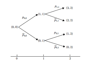
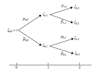
Let us move one step further and consider the binomial tree model up to two time steps, as shown in Figure 2.2, where each pair of numbers represents a state (which can be associated with the price of an asset if necessary). Out of each state at time $j$, two possible states are generated at time $j+1$. Hence, we have $2^{j}$ states at time $j$, starting with a single state at time 0 . The branching probabilities for reaching the next two states from one state, $(i, j)$, are $p_{i, j} \in[0,1]$ and $\bar{p}{i, j}=1-p{i, j}$, respectively. The collection of branching probabilities, $\mathbb{P}=\left{p_{i, j}, \bar{p}{i, j}\right}$, is again called a measure. As is shown in Figure 2.2, there are two paths over the time horizon from 0 to 1 , whereas there are four paths over the time horizon from 0 to 2 . The corresponding path probabilities for the horizon from 0 to 1 are $$ \pi{0,1}=\bar{p}{0,0} \quad \text { and } \quad \pi{1,1}=p_{0,0},
$$

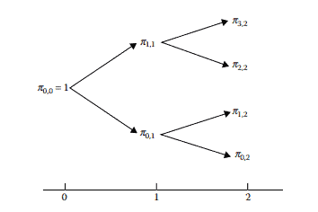
whereas for the horizon from 0 to 2 , they are
$$
\pi_{0,2}=\bar{p}{0,0} \bar{p}{0,1}, \pi_{1,2}=\bar{p}{0,0} p{0,1}, \pi_{2,2}=p_{0,0} \bar{p}{1,1} \text {, and } \pi{3,2}=p_{0,0} p_{1,1} \text {. }
$$
The path probabilities can also be marked in a binomial tree as is shown in Figure 2.3.

Consider now another set of branching probabilities, $\mathbb{Q}=\left{q_{i, j}, \bar{q}{i, j}=\right.$ $\left.1-q{i, j}\right}$, for the same tree. The corresponding path probabilities are
$$
\pi_{0,1}^{\prime}=\bar{q}{0,0} \quad \text { and } \quad \pi{1,1}^{\prime}=q_{0,0}
$$
up to time 1 , and
$$
\pi_{0,2}^{\prime}=\bar{q}{0,0} \bar{q}{0,1}, \pi_{1,2}^{\prime}=\bar{q}{0,0} q{0,1}, \pi_{2,2}^{\prime}=q_{0,0} \bar{q}{1,1} \text {, and } \pi{3,2}^{\prime}=q_{0,0} q_{1,1}
$$
up to time 2. Suppose that the $\mathbb{P}$-probability of paths $\pi_{i, j} \neq 0$ for all $i, j$. We then can define the ratio of path probabilities as follows:
$$
\zeta_{i, j}=\frac{\pi_{i, j}^{\prime}}{\pi_{i, j}} .
$$

金融代写|利率建模代写Interest Rate Modeling代考|ACTL40004

利率建模代考

金融代写|利率建模代写Interest Rate Modeling代考|MARTINGALES

本章最后介绍了鞅,这是导数建模中的一个关键概念。定义如下。
定义1.5一个随机过程, $M_{t}$ ,称为 $\mathbb{P}$-martingale 当且仅当它具有以下属性:

  1. $E^{\mathbb{P}}\left[\left|M_{t}\right|\right]<\infty, \quad \forall t$
  2. $E^{\mathbb{P}}\left[M_{t} \mid \mathcal{F}{s}\right]=M s, \quad \forall s \leq t$ 鞅属性与投资或投机中的公平游戏有关。让我们想想 $M{t}-M_{s}$ 作为两方在一段时间内赌博的损益 $(\mathrm{P} \backslash \& \mathrm{Q})(s, t)$. 如 果预期盈亏为零,则认为该游戏是公平的。日常生活中公平游戏的例子包括抛硬币游戏和金融市场的期货投傝。在 数学中,也有很茤例子。事实上,到目前为止,我们已经看到了其中的几个,我们在下面提酲读者。
    例子 $1.4$
  3. 简单的随机游走, $X_{n}$, 是鞅,因为 $E\left[\left|X_{n}\right|\right]<n \sqrt{\Delta t}$ 和 $E\left[X_{n} \mid \mathcal{F} m\right]=X m, m \leq n$
    $\mathrm{~ 2 . ~ 一 个 巴}$
  4. 随机积分 $X_{t}=\int_{0}^{t} f(u) \mathrm{d} W_{u}$ 是鞅,因为
    $$
    E^{P}\left[X_{t} \mid \mathcal{F} s\right]=E^{P}\left[\int 0^{s}+\int_{s}^{t} f(u) \mathrm{d} W_{u} \mid \mathcal{F}{s}\right] \quad=\int 0^{s} f(u) \mathrm{d} W{u}=X_{s}, \quad \forall s \leq t
    $$
    在这里,我们应用了随机积分的第一个性质(参见第 11 页)。
  5. 过程 $M_{t}=\exp \left(\int_{0}^{t} \sigma_{s} \mathrm{~d} W_{s}-\frac{1}{2} \sigma_{s}^{2} \mathrm{~d} s\right)$ 是指数鞅。事实上,使用伊藤引理,我们可以证明
    $$
    \mathrm{d} M_{t}=\sigma_{t} M_{t} \mathrm{~d} W_{t}
    $$
    这是一个没有漂移的伊藤工艺。它曎循
    $$
    M_{t}=M_{s}+\int_{s}^{t} M_{u} \sigma_{u} \mathrm{~d} W_{u}
    $$
    根据上一个例子的结论,我们知道 $M_{t}$ 是鞅。
    我们在此强调,Ito 过程是鞅过程当且仅当其漂移项为零。最后,我们提出两个额外的例子。

金融代写|利率建模代写Interest Rate Modeling代考|A Motivating Example

考虑最简单的期权定价模型,标的资产邅唕一个周期的二项式过程,如图 $2.1$ 所示。如图 $2.1,0 \leq p \leq 1$ 和 $\bar{p}=1-p$. 期权的时间收益 $1, f\left(S_{u}\right)$ 和 $f\left(S_{d}\right)$, 是明确给出的,我们想要确定 $f(S)$ ,期权在时间 0 的价值。不失一般性,我们假设 模型中的利率为零。为了避免套利,我们必须强加命令 $S_{d} \leq S \leq S_{u}$. 我们称之为 $\mathbb{P}=p, \bar{p}$ 底层过程的客观度量。 根据预期对期权定价可能很诱人 $\mathbb{P}$ :
$$
f(S)=E^{\mathbb{P}}\left[f\left(S_{1}\right)\right] \quad=p f\left(S_{u}\right)+\bar{p} f\left(S_{d}\right)
$$
但是,除了特殊的 $p$ ,上述价格产生套利,因此是错误的。为了看到这一点,我们在时间复制期权的收益 $l$ 使用标的资产 和现金债券的投资组合,以及相应的单位数量, $\alpha$ 和 $\beta$ ,这样,在时间 1 ,
$$
\alpha S_{u}+\beta=f\left(S_{u}\right) \quad \alpha S_{d}+\beta=f\left(S_{d}\right)
$$
解决 $\alpha$ 和 $\beta ,$ 我们获得
$$
\alpha=\frac{f\left(S_{u}\right)-f\left(S_{d}\right)}{S_{u}-S_{d}}, \beta=\frac{S_{u} f\left(S_{d}\right)-S_{d} f\left(S_{u}\right)}{S_{u}-S_{d}}
$$
方程 $2.2$ 意味着投资组合和期权的时间 1 值是相同的。为了避免套利,它们在时间 0 的值也必须相同, ${ }^{*}$ 在时间 0 产生期 权的套利价格:
$$
f(S)=\alpha S+\beta \quad=q f\left(S_{u}\right)+\bar{q} f\left(S_{d}\right)=E^{\mathbb{Q}}\left[f\left(S_{1}\right)\right]
$$
在哪里 $\mathbb{Q}=q, \bar{q}, \quad$ 和
$$
q=\frac{S-S_{d}}{S_{u}-S_{d}}, \quad \bar{q}=1-q
$$
是一组不同的概率。请注意,方程 $2.4$ 给出期权的无套利价格。任何其他价格都会引起市场套利。因此,方程 $2.1$ 中的期 望价格是正确的,仅当 $p=q .$ 实际上, $q, \bar{q}$ 是唯一满足的概率集
$$
S=q S_{u}+\bar{q} S_{d}=E^{\mathbb{Q}}\left(S_{1}\right)
$$

金融代写|利率建模代写Interest Rate Modeling代考|Binomial Trees and Path Probabilities

让我们进一步考虑二叉树模型最多两个时间步长,如图 $2.2$ 所示,其中每对数字代表一个状态(必要时可以与资产价格 相关联)。离开每个州的时间 $j$ ,在时间产生两种可能的状态 $j+1$. 因此,我们有 $2^{j}$ 当时的状态 $j$ ,从时间 0 的单个状态 开始。从一个状态到达下两个状态的分支概率, $(i, j)$ , 是 $p_{i, j} \in[0,1]$ 和 $\bar{p} i, j=1-p i, j$ ,分别。分支概率的集合,
Imathbb{P}=\left{p_{i, j}, Vbar{p}{,j}}rright} , 又称为测度。如图 $2.2$ 所示,在从 0 到 1 的时间范围内有两条路径,而在从 0 到 2 的时间范围内有四条路径。地平线从 0 到 1 的相应路径概率为
$$
\pi 0,1=\bar{p} 0,0 \quad \text { and } \quad \pi 1,1=p_{0,0},
$$
而对于从 0 到 2 的地平线,它们是
$$
\pi_{0,2}=\bar{p} 0,0 \bar{p} 0,1, \pi_{1,2}=\bar{p} 0,0 p 0,1, \pi_{2,2}=p_{0,0} \bar{p} 1,1, \text { and } \pi 3,2=p_{0,0} p_{1,1} .
$$
路径概率也可以在二叉树中标记,如图 $2.3$ 所示。
$\mathrm{~ 现 在 考 虑 另 一 组 分 支 概 率 , ~ I m a t h b b { Q } = \ l e f t { q _ { i , j } , \ b a r { q } { i , j } =}$ 概率是
$$
\pi_{0,1}^{\prime}=\bar{q} 0,0 \quad \text { and } \quad \pi 1,1^{\prime}=q_{0,0}
$$
直到时间 1 ,和
$$
\pi_{0,2}^{\prime}=\bar{q} 0,0 \bar{q} 0,1, \pi_{1,2}^{\prime}=\bar{q} 0,0 q 0,1, \pi_{2,2}^{\prime}=q_{0,0} \bar{q} 1,1, \text { and } \pi 3,2^{\prime}=q_{0,0} q_{1,1}
$$
到时间 2 . 假设 $\mathbb{P}$ – 路径概率 $\pi_{i, j} \neq 0$ 对所有人 $i, j$. 然后我们可以定义路径概率的比率如下:
$$
\zeta_{i, j}=\frac{\pi_{i, j}^{\prime}}{\pi_{i, j}} .
$$

金融代写|利率建模代写Interest Rate Modeling代考 请认准statistics-lab™

统计代写请认准statistics-lab™. statistics-lab™为您的留学生涯保驾护航。

金融工程代写

金融工程是使用数学技术来解决金融问题。金融工程使用计算机科学、统计学、经济学和应用数学领域的工具和知识来解决当前的金融问题,以及设计新的和创新的金融产品。

非参数统计代写

非参数统计指的是一种统计方法,其中不假设数据来自于由少数参数决定的规定模型;这种模型的例子包括正态分布模型和线性回归模型。

广义线性模型代考

广义线性模型(GLM)归属统计学领域,是一种应用灵活的线性回归模型。该模型允许因变量的偏差分布有除了正态分布之外的其它分布。

术语 广义线性模型(GLM)通常是指给定连续和/或分类预测因素的连续响应变量的常规线性回归模型。它包括多元线性回归,以及方差分析和方差分析(仅含固定效应)。

有限元方法代写

有限元方法(FEM)是一种流行的方法,用于数值解决工程和数学建模中出现的微分方程。典型的问题领域包括结构分析、传热、流体流动、质量运输和电磁势等传统领域。

有限元是一种通用的数值方法,用于解决两个或三个空间变量的偏微分方程(即一些边界值问题)。为了解决一个问题,有限元将一个大系统细分为更小、更简单的部分,称为有限元。这是通过在空间维度上的特定空间离散化来实现的,它是通过构建对象的网格来实现的:用于求解的数值域,它有有限数量的点。边界值问题的有限元方法表述最终导致一个代数方程组。该方法在域上对未知函数进行逼近。[1] 然后将模拟这些有限元的简单方程组合成一个更大的方程系统,以模拟整个问题。然后,有限元通过变化微积分使相关的误差函数最小化来逼近一个解决方案。

tatistics-lab作为专业的留学生服务机构,多年来已为美国、英国、加拿大、澳洲等留学热门地的学生提供专业的学术服务,包括但不限于Essay代写,Assignment代写,Dissertation代写,Report代写,小组作业代写,Proposal代写,Paper代写,Presentation代写,计算机作业代写,论文修改和润色,网课代做,exam代考等等。写作范围涵盖高中,本科,研究生等海外留学全阶段,辐射金融,经济学,会计学,审计学,管理学等全球99%专业科目。写作团队既有专业英语母语作者,也有海外名校硕博留学生,每位写作老师都拥有过硬的语言能力,专业的学科背景和学术写作经验。我们承诺100%原创,100%专业,100%准时,100%满意。

随机分析代写


随机微积分是数学的一个分支,对随机过程进行操作。它允许为随机过程的积分定义一个关于随机过程的一致的积分理论。这个领域是由日本数学家伊藤清在第二次世界大战期间创建并开始的。

时间序列分析代写

随机过程,是依赖于参数的一组随机变量的全体,参数通常是时间。 随机变量是随机现象的数量表现,其时间序列是一组按照时间发生先后顺序进行排列的数据点序列。通常一组时间序列的时间间隔为一恒定值(如1秒,5分钟,12小时,7天,1年),因此时间序列可以作为离散时间数据进行分析处理。研究时间序列数据的意义在于现实中,往往需要研究某个事物其随时间发展变化的规律。这就需要通过研究该事物过去发展的历史记录,以得到其自身发展的规律。

回归分析代写

多元回归分析渐进(Multiple Regression Analysis Asymptotics)属于计量经济学领域,主要是一种数学上的统计分析方法,可以分析复杂情况下各影响因素的数学关系,在自然科学、社会和经济学等多个领域内应用广泛。

MATLAB代写

MATLAB 是一种用于技术计算的高性能语言。它将计算、可视化和编程集成在一个易于使用的环境中,其中问题和解决方案以熟悉的数学符号表示。典型用途包括:数学和计算算法开发建模、仿真和原型制作数据分析、探索和可视化科学和工程图形应用程序开发,包括图形用户界面构建MATLAB 是一个交互式系统,其基本数据元素是一个不需要维度的数组。这使您可以解决许多技术计算问题,尤其是那些具有矩阵和向量公式的问题,而只需用 C 或 Fortran 等标量非交互式语言编写程序所需的时间的一小部分。MATLAB 名称代表矩阵实验室。MATLAB 最初的编写目的是提供对由 LINPACK 和 EISPACK 项目开发的矩阵软件的轻松访问,这两个项目共同代表了矩阵计算软件的最新技术。MATLAB 经过多年的发展,得到了许多用户的投入。在大学环境中,它是数学、工程和科学入门和高级课程的标准教学工具。在工业领域,MATLAB 是高效研究、开发和分析的首选工具。MATLAB 具有一系列称为工具箱的特定于应用程序的解决方案。对于大多数 MATLAB 用户来说非常重要,工具箱允许您学习应用专业技术。工具箱是 MATLAB 函数(M 文件)的综合集合,可扩展 MATLAB 环境以解决特定类别的问题。可用工具箱的领域包括信号处理、控制系统、神经网络、模糊逻辑、小波、仿真等。

R语言代写问卷设计与分析代写
PYTHON代写回归分析与线性模型代写
MATLAB代写方差分析与试验设计代写
STATA代写机器学习/统计学习代写
SPSS代写计量经济学代写
EVIEWS代写时间序列分析代写
EXCEL代写深度学习代写
SQL代写各种数据建模与可视化代写

金融代写|利率建模代写Interest Rate Modeling代考|ACTL90003

如果你也在 怎样代写利率建模Interest Rate Modeling这个学科遇到相关的难题,请随时右上角联系我们的24/7代写客服。

利率模型是指一种对利率的运动和演变进行建模的数学方法。它是一种基于市场风险的单因素短利率模型。瓦西克利率模型常用于经济学中,以确定利率在未来的移动方向。

statistics-lab™ 为您的留学生涯保驾护航 在代写利率建模Interest Rate Modeling方面已经树立了自己的口碑, 保证靠谱, 高质且原创的统计Statistics代写服务。我们的专家在代写利率建模Interest Rate Modeling代写方面经验极为丰富,各种代写利率建模Interest Rate Modeling相关的作业也就用不着说。

我们提供的利率建模Interest Rate Modeling及其相关学科的代写,服务范围广, 其中包括但不限于:

  • Statistical Inference 统计推断
  • Statistical Computing 统计计算
  • Advanced Probability Theory 高等概率论
  • Advanced Mathematical Statistics 高等数理统计学
  • (Generalized) Linear Models 广义线性模型
  • Statistical Machine Learning 统计机器学习
  • Longitudinal Data Analysis 纵向数据分析
  • Foundations of Data Science 数据科学基础
金融代写|利率建模代写Interest Rate Modeling代考|ACTL90003

金融代写|利率建模代写Interest Rate Modeling代考|Simple Random Walks

Simple random walks are discrete time series, $\left{X_{i}\right}$, defined as
$$
\begin{aligned}
X_{0} &=0, \
X_{n+1} &= \begin{cases}X_{n}-\sqrt{\Delta t}, & p=\frac{1}{2} \
X_{n}+\sqrt{\Delta t}, & 1-p=\frac{1}{2}\end{cases}
\end{aligned}
$$
where $\Delta t>0$ stands for the interval of time for stepping forward. One can verify that $\left{X_{i}\right}$ have the following properties:

  1. The increment of $X_{n+1}-X_{n}$ is independent of $\left{X_{i}\right}, \forall i \leq n$.
  2. $E\left[X_{n} \mid X_{m}\right]=X_{m}, m \leq n$.
  3. $\operatorname{Var}\left[X_{n} \mid X_{m}\right]=(n-m) \Delta t, m \leq n$.
    An interesting feature of the simple random walk is the linearity of $X_{i}$ ‘s variance in time: given $X_{0}$, the variance of $X_{i}$ is equal to $i \Delta t$, the time it takes the time series to evolve from $X_{0}$ to $X_{i}$.

Out of the simple Brownian random walk, we can construct a continuous-time process through linear interpolation:
$$
\bar{X}(t)=X_{i}+\frac{t-i \Delta t}{\Delta t}\left(X_{i+1}-X_{i}\right), \quad t \in[i \Delta t,(i+1) \Delta t]
$$
We are interested in the limiting process of $\bar{X}(t)$ as $\Delta t \rightarrow 0$, in the hope that the limit remains a meaningful stochastic process. The next theorem confirms just that.

金融代写|利率建模代写Interest Rate Modeling代考|Brownian Motion

A continuous stochastic process is a collection of real-valued random variables, ${X(t, \omega), 0 \leq t \leq T}$ or $\left{X_{t}(\omega), 0 \leq t \leq T\right}$, that are defined on a probability space $(\Omega, \mathcal{F}, \mathbb{P})$. Here $\Omega$ is the collection of all $\omega$ s, which are so-called sample points, $\mathcal{F}$ the smallest $\sigma$-algebra that contains $\Omega$, and $\mathbb{P}$ a probability measure on $\Omega$. Each random outcome, $\omega \in \Omega$, corresponds to an entire time series
$$
t \rightarrow X_{t}(\omega), \quad t \in T
$$
which is called a path of $X_{t}$. In view of Equation 1.7, we can regard $X_{t}(\omega)$ as a function of two variables, $\omega$ and $t$. For notational simplicity, however, we often suppress the $\omega$ variable when its explicit appearance is not necessary.

In the context of financial modeling, we are particularly interested in the Brownian motion introduced earlier. Its formal definition is given below.

Definition 1.1 A Brownian motion or a Wiener process is a realvalued stochastic process, $W_{t}$ or $W(t), 0 \leq t \leq \infty$, that has the following properties:

  1. $W(0)=0$.
  2. $W(t+s)-W(t)$ is independent of ${W(u), 0 \leq u \leq t}$.
  3. For $t \geq 0$ and $s>0$, the increment $W(t+s)-W(t) \sim N(0, s)$.
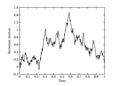
  4. $W(t)$ is continuous almost surely (a.s.).
    Here $N(0, s)$ stands for a normal distribution with mean zero and variance s. Note that in some literature, property 4 is not part of the definition, as it can be proved to be implied by the first three properties (Varadhan, $1980 \mathrm{a}$ or Ikeda and Watanabe, 1989). A sample path of $W(t)$ is shown in Figure $1.1$, which is generated with a step size of $\Delta t=2^{-10}$.

Brownian motion plays a major role in continuous time stochastic modeling in physics, engineering and finance. In finance, it has been used to model the random behavior of asset returns. Several major properties of Brownian motion are listed below.

金融代写|利率建模代写Interest Rate Modeling代考|STOCHASTIC INTEGRALS

Stochastic calculus considers the integration and differentiation of general $\mathcal{F}{t}$-adaptive functions. The purpose of developing such a stochastic calculus is to model financial time series (with random dynamics) with either integral or differential equations. According to Lemma 1.1, a Brownian motion, $W(t)$, is nowhere differentiable in the usual sense of differentiation for deterministic functions. To define differentials of stochastic processes in a proper sense, we must first study the notion of stochastic integrals. Stochastic integrals can be defined for functions in the square-integrable space, $H^{2}[0, T]=L^{2}(\Omega \times[0, T], \mathrm{d} \mathbb{P} \times \mathrm{d} t)$, which is defined to be the collection of functions satisfying $$ E\left[\int{0}^{T}|f(t, \omega)|^{2} \mathrm{~d} t\right]<\infty
$$
Note that, without indicated otherwise, $E[\cdot]$ means $E^{\mathbb{P}}[\cdot]$, the unconditional expectation under $\mathbb{P}$. The definition consists of a three-step procedure. First, we make the definition for elementary or piecewise constant functions in an intuitive way. Second, we define the integrals of a bounded continuous function as a limit of integrals of elementary functions. Finally, we define the integral of a general square-integrable function as a limit of integrals of bounded continuous functions. The key in this three-step procedure is of course to ensure the convergence of the limits in $L^{2}(\Omega, \mathcal{F}, \mathbb{P})$, the Hilbert space of random variables satisfying
$$
E\left[X^{2}(\omega)\right]<\infty
$$
This definition approach is taken by Oksendal (1992). Alternative treatments of course also exist; see, for example, Mikosch (1998).

金融代写|利率建模代写Interest Rate Modeling代考|ACTL90003

利率建模代考

金融代写|利率建模代写Interest Rate Modeling代考|Simple Random Walks

简单的随机游走是离散的时间序列, left{X_{i}}right }, 定义为
$$
X_{0}=0, X_{n+1} \quad=\left{X_{n}-\sqrt{\Delta t}, \quad p=\frac{1}{2} X_{n}+\sqrt{\Delta t}, \quad 1-p=\frac{1}{2}\right.
$$
在哪里 $\Delta t>0$ 代表前进的时间间隔。可以验证 lleft{X_{i}}right} $}$ 具有以下属性:

  1. 的增量 $X_{n+1}-X_{n}$ 独立于⿴left $\left{X_{-}{i} \backslash\right.$ Iight}, Iforall i leq n.
  2. $E\left[X_{n} \mid X_{m}\right]=X_{m}, m \leq n$.
  3. $\operatorname{Var}\left[X_{n} \mid X_{m}\right]=(n-m) \Delta t, m \leq n$.
    简单随机游走的一个有趣特征是 $X_{i}$ 的时间变化: 给定 $X_{0}$, 的方差 $X_{i}$ 等于 $i \Delta t$, 时间序列从 $X_{0}$ 至 $X_{i}$.
    从简单的布朗随机游走中,我们可以通过线性揷值构造一个连续时间的过程:
    $$
    \bar{X}(t)=X_{i}+\frac{t-i \Delta t}{\Delta t}\left(X_{i+1}-X_{i}\right), \quad t \in[i \Delta t,(i+1) \Delta t]
    $$
    我们对限制过程感兴趣 $\bar{X}(t)$ 作为 $\Delta t \rightarrow 0$ ,希望极限仍然是一个有意义的随机过程。下一个定理证实了这一点。

金融代写|利率建模代写Interest Rate Modeling代考|Brownian Motion

连续随机过程是实值随机变量的集合, $X(t, \omega), 0 \leq t \leq T$ 或者 Ueft $\left{X_{-} \mathrm{~ { t } (}\right.$ 间上定义 $(\Omega, \mathcal{F}, \mathbb{P})$. 这里 $\Omega$ 是所有的集合 $\omega \mathrm{s}$ ,即所谓的样本点, $\mathcal{F}$ 最小的 $\sigma$-代数包含 $\Omega$ ,和 $\mathbb{P}$ 概率测度 $\Omega$. 每个随 机结果, $\omega \in \Omega$ ,对应于整个时间序列
$$
t \rightarrow X_{t}(\omega), \quad t \in T
$$
这被称为路径 $X_{t}$. 鉴于公式 1.7,我们可以认为 $X_{t}(\omega)$ 作为两个变量的函数, $\omega$ 和 $t$. 然而,为了符号的简单性,我 们经常抑制 $\omega$ 不需要显式外观时的变量。
在金融建模的背景下,我们对前面介绍的布朗运动特别感兴趣。其正式定义如下。
定义 $1.1$ 布朗运动或维纳过程是实值随机过程, $W_{t}$ 或者 $W(t), 0 \leq t \leq \infty$ ,具有以下性质:

  1. $W(0)=0$.
  2. $W(t+s)-W(t)$ 独立于 $W(u), 0 \leq u \leq t$.
  3. 为了 $t \geq 0$ 和 $s>0$, 增量 $W(t+s)-W(t) \sim N(0, s)$.
  4. $W(t)$ 几平肯定是连续的 (as)。
    这里 $N(0, s)$ 代表均值为零且方差为 $\mathrm{s}$ 的正态分布。请注意,在某些文献中,属性 4 不是定义的一部分,因 为可以证明前三个属性暗示了它 (Varadhan,1980a或池田和渡边,1989) 。一个示例路径 $W(t)$ 如图1.1 ,它的生成步长为 $\Delta t=2^{-10}$.
    布朗运动在物理学、工程和金融领域的连续时间随机建模中发挥着重要作用。在金融领域,它已被用于模拟资产回 报的随机行为。下面列出了布朗运动的几个主要性质。

金融代写|利率建模代写Interest Rate Modeling代考|STOCHASTIC INTEGRALS

随机微积分考虑一般的积分和微分 $\mathcal{F} t$ – 自适应功能。开发这种随机微积分的目的是用积分或微分方程对金融时间序 列 (具有随机动力学) 进行建模。根据引理 1.1,布朗运动, $W(t)$ ,在确定性函数的通常微分意义上是不可微的。 为了正确定义随机过程的微分,我们必须首先研究随机积分的概念。可以为平方可积空间中的函数定义随机积分, $H^{2}[0, T]=L^{2}(\Omega \times[0, T], \mathrm{d} \mathbb{P} \times \mathrm{d} t)$ ,它被定义为满足的函数的集合
$$
E\left[\int 0^{T}|f(t, \omega)|^{2} \mathrm{~d} t\right]<\infty
$$
请注意,在没有另外说明的情况下, $E[\cdot]$ 方法 $E^{\mathbb{P}}[\cdot]$, 下的无条件期望 $\mathbb{P}$. 该定义包括一个三步程序。首先,我们以 直观的方式定义基本或分段常数函数。其次,我们将有界连续函数的积分定义为初等函数积分的极限。最后,我们 将一般平方可积函数的积分定义为有界连续函数积分的极限。这个三步程序的关键当然是确保在 $L^{2}(\Omega, \mathcal{F}, \mathbb{P})$ ,随 机变量的希尔伯特空间满足
$$
E\left[X^{2}(\omega)\right]<\infty
$$
Oksendal (1992) 采用了这种定义方法。当然也存在替代疗法;例如,参见 Mikosch (1998)。

金融代写|利率建模代写Interest Rate Modeling代考 请认准statistics-lab™

统计代写请认准statistics-lab™. statistics-lab™为您的留学生涯保驾护航。

金融工程代写

金融工程是使用数学技术来解决金融问题。金融工程使用计算机科学、统计学、经济学和应用数学领域的工具和知识来解决当前的金融问题,以及设计新的和创新的金融产品。

非参数统计代写

非参数统计指的是一种统计方法,其中不假设数据来自于由少数参数决定的规定模型;这种模型的例子包括正态分布模型和线性回归模型。

广义线性模型代考

广义线性模型(GLM)归属统计学领域,是一种应用灵活的线性回归模型。该模型允许因变量的偏差分布有除了正态分布之外的其它分布。

术语 广义线性模型(GLM)通常是指给定连续和/或分类预测因素的连续响应变量的常规线性回归模型。它包括多元线性回归,以及方差分析和方差分析(仅含固定效应)。

有限元方法代写

有限元方法(FEM)是一种流行的方法,用于数值解决工程和数学建模中出现的微分方程。典型的问题领域包括结构分析、传热、流体流动、质量运输和电磁势等传统领域。

有限元是一种通用的数值方法,用于解决两个或三个空间变量的偏微分方程(即一些边界值问题)。为了解决一个问题,有限元将一个大系统细分为更小、更简单的部分,称为有限元。这是通过在空间维度上的特定空间离散化来实现的,它是通过构建对象的网格来实现的:用于求解的数值域,它有有限数量的点。边界值问题的有限元方法表述最终导致一个代数方程组。该方法在域上对未知函数进行逼近。[1] 然后将模拟这些有限元的简单方程组合成一个更大的方程系统,以模拟整个问题。然后,有限元通过变化微积分使相关的误差函数最小化来逼近一个解决方案。

tatistics-lab作为专业的留学生服务机构,多年来已为美国、英国、加拿大、澳洲等留学热门地的学生提供专业的学术服务,包括但不限于Essay代写,Assignment代写,Dissertation代写,Report代写,小组作业代写,Proposal代写,Paper代写,Presentation代写,计算机作业代写,论文修改和润色,网课代做,exam代考等等。写作范围涵盖高中,本科,研究生等海外留学全阶段,辐射金融,经济学,会计学,审计学,管理学等全球99%专业科目。写作团队既有专业英语母语作者,也有海外名校硕博留学生,每位写作老师都拥有过硬的语言能力,专业的学科背景和学术写作经验。我们承诺100%原创,100%专业,100%准时,100%满意。

随机分析代写


随机微积分是数学的一个分支,对随机过程进行操作。它允许为随机过程的积分定义一个关于随机过程的一致的积分理论。这个领域是由日本数学家伊藤清在第二次世界大战期间创建并开始的。

时间序列分析代写

随机过程,是依赖于参数的一组随机变量的全体,参数通常是时间。 随机变量是随机现象的数量表现,其时间序列是一组按照时间发生先后顺序进行排列的数据点序列。通常一组时间序列的时间间隔为一恒定值(如1秒,5分钟,12小时,7天,1年),因此时间序列可以作为离散时间数据进行分析处理。研究时间序列数据的意义在于现实中,往往需要研究某个事物其随时间发展变化的规律。这就需要通过研究该事物过去发展的历史记录,以得到其自身发展的规律。

回归分析代写

多元回归分析渐进(Multiple Regression Analysis Asymptotics)属于计量经济学领域,主要是一种数学上的统计分析方法,可以分析复杂情况下各影响因素的数学关系,在自然科学、社会和经济学等多个领域内应用广泛。

MATLAB代写

MATLAB 是一种用于技术计算的高性能语言。它将计算、可视化和编程集成在一个易于使用的环境中,其中问题和解决方案以熟悉的数学符号表示。典型用途包括:数学和计算算法开发建模、仿真和原型制作数据分析、探索和可视化科学和工程图形应用程序开发,包括图形用户界面构建MATLAB 是一个交互式系统,其基本数据元素是一个不需要维度的数组。这使您可以解决许多技术计算问题,尤其是那些具有矩阵和向量公式的问题,而只需用 C 或 Fortran 等标量非交互式语言编写程序所需的时间的一小部分。MATLAB 名称代表矩阵实验室。MATLAB 最初的编写目的是提供对由 LINPACK 和 EISPACK 项目开发的矩阵软件的轻松访问,这两个项目共同代表了矩阵计算软件的最新技术。MATLAB 经过多年的发展,得到了许多用户的投入。在大学环境中,它是数学、工程和科学入门和高级课程的标准教学工具。在工业领域,MATLAB 是高效研究、开发和分析的首选工具。MATLAB 具有一系列称为工具箱的特定于应用程序的解决方案。对于大多数 MATLAB 用户来说非常重要,工具箱允许您学习应用专业技术。工具箱是 MATLAB 函数(M 文件)的综合集合,可扩展 MATLAB 环境以解决特定类别的问题。可用工具箱的领域包括信号处理、控制系统、神经网络、模糊逻辑、小波、仿真等。

R语言代写问卷设计与分析代写
PYTHON代写回归分析与线性模型代写
MATLAB代写方差分析与试验设计代写
STATA代写机器学习/统计学习代写
SPSS代写计量经济学代写
EVIEWS代写时间序列分析代写
EXCEL代写深度学习代写
SQL代写各种数据建模与可视化代写

金融代写|利率建模代写Interest Rate Modeling代考|MATH4513

如果你也在 怎样代写利率建模Interest Rate Modeling这个学科遇到相关的难题,请随时右上角联系我们的24/7代写客服。

利率模型是指一种对利率的运动和演变进行建模的数学方法。它是一种基于市场风险的单因素短利率模型。瓦西克利率模型常用于经济学中,以确定利率在未来的移动方向。

statistics-lab™ 为您的留学生涯保驾护航 在代写利率建模Interest Rate Modeling方面已经树立了自己的口碑, 保证靠谱, 高质且原创的统计Statistics代写服务。我们的专家在代写利率建模Interest Rate Modeling代写方面经验极为丰富,各种代写利率建模Interest Rate Modeling相关的作业也就用不着说。

我们提供的利率建模Interest Rate Modeling及其相关学科的代写,服务范围广, 其中包括但不限于:

  • Statistical Inference 统计推断
  • Statistical Computing 统计计算
  • Advanced Probability Theory 高等概率论
  • Advanced Mathematical Statistics 高等数理统计学
  • (Generalized) Linear Models 广义线性模型
  • Statistical Machine Learning 统计机器学习
  • Longitudinal Data Analysis 纵向数据分析
  • Foundations of Data Science 数据科学基础
金融代写|利率建模代写Interest Rate Modeling代考|MATH4513

金融代写|利率建模代写Interest Rate Modeling代考|Discretization of Forward Rate Process

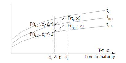
We recall the forward rate process in the H.JM model as
$$
\begin{aligned}
f(t, T)=& f(0, T)+\int_{0}^{t}\left{-\sigma(s, T) v(s, T)+\sigma(s, T) \varphi_{s}\right} d s \
&+\int_{0}^{t} \sigma(s, T) d W_{s}
\end{aligned}
$$
where $W_{t}$ is a $d$-dimensional P-Brownian motion. The HJM model is called Gaussian if $\sigma(t, T)$ is a deterministic function of $t$ and $T$. In this book, we always assume that volatility $\sigma(t, T)$ is deterministic and continuous with respect to $t$ and $T$. Then, $v(t, T)$ is also deterministic and continuous. In the following, the market price of risk is assumed to be constant. The validity of the constancy assumption will be examined in the context of risk management in Chapter $7 .$
Data observation
Denoting the market price of risk as a constant $\varphi$, the above forward rate process is expressed by
$$
\begin{aligned}
f(t, T)=& f(0, T)+\int_{0}^{t}{-\sigma(s, T) v(s, T)+\sigma(s, T) \varphi} d s \
&+\int_{0}^{t} \sigma(s, T) d W_{s} .
\end{aligned}
$$
Next, we specify a historical dataset as follows. Let a time interval $\Delta t>0$ be fixed, and $\left{t_{k}\right}_{k=1, \cdots, J+1}$ be a sequence of observation dates such that $t_{1}=0$ and $t_{k+1}-t_{k}=\Delta t$, where $J+1$ is the number of observation times. We denote the time length to a maturity $T$ from $t$ by $x=T-t$. For an integer $n \geq d$, $x_{1}, \cdots, x_{n}$ denotes a sequence of time lengths to maturity.

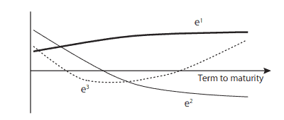
Typically, we observe the instantaneous forward rate $F\left(t_{k}, x_{i}\right)$ with respect to fixed $x_{i}$. Fig. $6.1$ illustrates an example of forward rate curves observed at $t_{k}, t_{k+1}$, and $t_{k+2}$, showing $F\left(t_{k}, x_{i}\right), F\left(t_{k+1}, x_{i}-\Delta t\right)$, and so on. We assume that the dynamics of these observations follow equation (6.2).

金融代写|利率建模代写Interest Rate Modeling代考|Estimation of Market Price of Risk

We recall the volatility structure associated with PCA in Section 4.3. A sample covariance matrix $V$ is defined by
$$
\begin{aligned}
V_{i j}=& \frac{1}{\Delta t} \operatorname{Cov}\left(F\left(t_{k}+\Delta t, x_{i}-\Delta t\right)-F\left(t_{k}, x_{i}\right)\right.\
&\left.F\left(t_{k}+\Delta t, x_{j}-\Delta t\right)-F\left(t_{k}, x_{j}\right)\right) ; \quad i, j=1, \cdots, n .
\end{aligned}
$$
We assume that $V$ has rank $d \leq n$. By the argument in Appendix $\mathrm{B}$, the covariance matrix is decomposed into $V_{i j}=\sum_{l=1}^{d} e_{i}^{l} \rho_{l}^{2} e_{j}^{l}$ for $i, j \leq n$, where $\rho_{l}^{2}$ is the lth eigenvalue, and $e^{l}=\left(e_{1}^{l}, \cdots, e_{n}^{l}\right)^{T}$ is the $l$ th principal component of the covariance for $l=1, \cdots, d$.
We always assume that
$$
e_{1}^{l}>0, \quad \rho_{l}>0 ; \quad l=1, \cdots, d
$$
This assumption is significant in the interpretation of the meaning of the market price of risk in Sections $6.4$ and 6.5. Recall the equation (B.4), that is, that the principal components $e^{1}, \cdots, e^{d}$ form an orthonormal set. Thus,
$$
\sum_{i=1}^{n} e_{i}^{l} e_{i}^{h}=\delta_{l h} \quad ; \quad l, h=1, \cdots, d
$$

金融代写|利率建模代写Interest Rate Modeling代考|Market Price of Risk: State Space Setup

This section introduces another method to estimate the market price of risk: working in a state space.

Denoting the market price of risk by $\varphi^{\prime}=\left(\varphi_{1}^{\prime}, \cdots, \varphi_{d}^{\prime}\right)^{T}$, we return to the discretization as equation (6.13), which we reproduce below:
$$
\Delta F_{i}\left(t_{k}\right)=-\sigma_{0 i} v_{0 i} \Delta t+\sigma_{0 i} \varphi^{\prime} \Delta t+\sqrt{\Delta t} \sigma_{0 i} W_{1} ; i=1, \cdots, n, k=1, \cdots, J
$$
We remark that the volatility is assumed to be determined by a principal component. Our objective here is to directly obtain $\varphi^{\prime}$ from the above equations.
We denote by $\epsilon\left(\varphi^{\prime}\right)$ the sum of the squared difference between each side of equation $(6.26)$ in the time series and cross sections, neglecting the random part, such that
$$
\epsilon\left(\varphi^{\prime}\right)=\frac{1}{J} \sum_{k=1}^{J} \sum_{i=1}^{n}\left{\Delta F_{i}\left(t_{k}\right)+\left(\sigma_{0 i} v_{0 i}-\sigma_{0 i} \varphi^{\prime}\right) \Delta t\right}^{2}
$$
Let $\varphi^{\prime}$ be the solution that minimizes $\epsilon\left(\varphi^{\prime}\right)$. We call this setting a state space setup, and call that used in the previous section a $P C A$ setup to distinguish between the two approaches. We note the implications of both definitions below.

  • $\varphi$ is the solution that minimizes $\theta_{l}\left(\varphi_{l}\right)$ in equation $(6.19)$ in the principal component space, and also is the maximum likelihood estimate.
  • $\varphi^{\prime}$ is the solution that minimizes $\epsilon\left(\varphi^{\prime}\right)$ of equation $(6.27)$ in the state space.
金融代写|利率建模代写Interest Rate Modeling代考|MATH4513

利率建模代考

金融代写|利率建模代写Interest Rate Modeling代考|Discretization of Forward Rate Process

我们将 H.JM 模型中的远期利率过程回忆为

\begin{对齐} f(t, T)=& f(0, T)+\int_{0}^{t}\left{-\sigma(s, T) v(s, T)+\sigma( s, T) \varphi_{s}\right} d s \ &+\int_{0}^{t} \sigma(s, T) d W_{s} \end{aligned}\begin{对齐} f(t, T)=& f(0, T)+\int_{0}^{t}\left{-\sigma(s, T) v(s, T)+\sigma( s, T) \varphi_{s}\right} d s \ &+\int_{0}^{t} \sigma(s, T) d W_{s} \end{aligned}
在哪里在吨是一个d维 P-布朗运动。如果 HJM 模型称为高斯模型σ(吨,吨)是一个确定性函数吨和吨. 在本书中,我们总是假设波动性σ(吨,吨)是确定的和连续的吨和吨. 然后,在(吨,吨)也是确定性和连续性的。在下文中,假设风险的市场价格是恒定的。恒常假设的有效性将在本章的风险管理背景下进行检验7.
数据观察
将风险的市场价格表示为常数披,上述远期汇率过程表示为

F(吨,吨)=F(0,吨)+∫0吨−σ(s,吨)在(s,吨)+σ(s,吨)披ds +∫0吨σ(s,吨)d在s.
接下来,我们指定一个历史数据集,如下所示。设一个时间间隔Δ吨>0被固定,并且\left{t_{k}\right}_{k=1, \cdots, J+1}\left{t_{k}\right}_{k=1, \cdots, J+1}是一系列观察日期,使得吨1=0和吨ķ+1−吨ķ=Δ吨, 在哪里Ĵ+1是观察次数。我们表示到成熟的时间长度吨从吨经过X=吨−吨. 对于整数n≥d, X1,⋯,Xn表示到期的时间长度序列。

通常,我们观察瞬时远期汇率F(吨ķ,X一世)相对于固定X一世. 如图。6.1举例说明观察到的远期利率曲线吨ķ,吨ķ+1, 和吨ķ+2, 显示F(吨ķ,X一世),F(吨ķ+1,X一世−Δ吨), 等等。我们假设这些观察的动力学遵循方程(6.2)。

金融代写|利率建模代写Interest Rate Modeling代考|Estimation of Market Price of Risk

我们回顾了第 4.3 节中与 PCA 相关的波动率结构。样本协方差矩阵在定义为

在一世j=1Δ吨这⁡(F(吨ķ+Δ吨,X一世−Δ吨)−F(吨ķ,X一世) F(吨ķ+Δ吨,Xj−Δ吨)−F(吨ķ,Xj));一世,j=1,⋯,n.
我们假设在有等级d≤n. 根据附录中的论点乙,协方差矩阵分解为在一世j=∑l=1d和一世lρl2和jl为了一世,j≤n, 在哪里ρl2是第 l 个特征值,并且和l=(和1l,⋯,和nl)吨是个l协方差的第 th 个主成分l=1,⋯,d.
我们总是假设

和1l>0,ρl>0;l=1,⋯,d
这一假设对解释风险市场价格的含义具有重要意义。6.4和 6.5。回想方程(B.4),即主成分和1,⋯,和d形成一个正交集。因此,

∑一世=1n和一世l和一世H=dlH;l,H=1,⋯,d

金融代写|利率建模代写Interest Rate Modeling代考|Market Price of Risk: State Space Setup

本节介绍另一种估计风险市场价格的方法:在状态空间中工作。

表示风险的市场价格披′=(披1′,⋯,披d′)吨,我们回到方程(6.13)的离散化,我们在下面重现:

ΔF一世(吨ķ)=−σ0一世在0一世Δ吨+σ0一世披′Δ吨+Δ吨σ0一世在1;一世=1,⋯,n,ķ=1,⋯,Ĵ
我们注意到,假设波动率由主成分决定。我们的目标是直接获得披′从上面的方程。
我们表示ε(披′)方程两边的平方差之和(6.26)在时间序列和横截面中,忽略随机部分,使得

\epsilon\left(\varphi^{\prime}\right)=\frac{1}{J} \sum_{k=1}^{J} \sum_{i=1}^{n}\left{\ Delta F_{i}\left(t_{k}\right)+\left(\sigma_{0 i} v_{0 i}-\sigma_{0 i} \varphi^{\prime}\right) \Delta t \对}^{2}\epsilon\left(\varphi^{\prime}\right)=\frac{1}{J} \sum_{k=1}^{J} \sum_{i=1}^{n}\left{\ Delta F_{i}\left(t_{k}\right)+\left(\sigma_{0 i} v_{0 i}-\sigma_{0 i} \varphi^{\prime}\right) \Delta t \对}^{2}
让披′是最小化的解决方案ε(披′). 我们将此设置称为状态空间设置,并将上一节中使用的称为 a磷C一个设置来区分这两种方法。我们注意到以下两个定义的含义。

  • 披是最小化的解决方案θl(披l)在等式中(6.19)在主成分空间中,也是最大似然估计。
  • 披′是最小化的解决方案ε(披′)方程的(6.27)在状态空间。
金融代写|利率建模代写Interest Rate Modeling代考 请认准statistics-lab™

统计代写请认准statistics-lab™. statistics-lab™为您的留学生涯保驾护航。

金融工程代写

金融工程是使用数学技术来解决金融问题。金融工程使用计算机科学、统计学、经济学和应用数学领域的工具和知识来解决当前的金融问题,以及设计新的和创新的金融产品。

非参数统计代写

非参数统计指的是一种统计方法,其中不假设数据来自于由少数参数决定的规定模型;这种模型的例子包括正态分布模型和线性回归模型。

广义线性模型代考

广义线性模型(GLM)归属统计学领域,是一种应用灵活的线性回归模型。该模型允许因变量的偏差分布有除了正态分布之外的其它分布。

术语 广义线性模型(GLM)通常是指给定连续和/或分类预测因素的连续响应变量的常规线性回归模型。它包括多元线性回归,以及方差分析和方差分析(仅含固定效应)。

有限元方法代写

有限元方法(FEM)是一种流行的方法,用于数值解决工程和数学建模中出现的微分方程。典型的问题领域包括结构分析、传热、流体流动、质量运输和电磁势等传统领域。

有限元是一种通用的数值方法,用于解决两个或三个空间变量的偏微分方程(即一些边界值问题)。为了解决一个问题,有限元将一个大系统细分为更小、更简单的部分,称为有限元。这是通过在空间维度上的特定空间离散化来实现的,它是通过构建对象的网格来实现的:用于求解的数值域,它有有限数量的点。边界值问题的有限元方法表述最终导致一个代数方程组。该方法在域上对未知函数进行逼近。[1] 然后将模拟这些有限元的简单方程组合成一个更大的方程系统,以模拟整个问题。然后,有限元通过变化微积分使相关的误差函数最小化来逼近一个解决方案。

tatistics-lab作为专业的留学生服务机构,多年来已为美国、英国、加拿大、澳洲等留学热门地的学生提供专业的学术服务,包括但不限于Essay代写,Assignment代写,Dissertation代写,Report代写,小组作业代写,Proposal代写,Paper代写,Presentation代写,计算机作业代写,论文修改和润色,网课代做,exam代考等等。写作范围涵盖高中,本科,研究生等海外留学全阶段,辐射金融,经济学,会计学,审计学,管理学等全球99%专业科目。写作团队既有专业英语母语作者,也有海外名校硕博留学生,每位写作老师都拥有过硬的语言能力,专业的学科背景和学术写作经验。我们承诺100%原创,100%专业,100%准时,100%满意。

随机分析代写


随机微积分是数学的一个分支,对随机过程进行操作。它允许为随机过程的积分定义一个关于随机过程的一致的积分理论。这个领域是由日本数学家伊藤清在第二次世界大战期间创建并开始的。

时间序列分析代写

随机过程,是依赖于参数的一组随机变量的全体,参数通常是时间。 随机变量是随机现象的数量表现,其时间序列是一组按照时间发生先后顺序进行排列的数据点序列。通常一组时间序列的时间间隔为一恒定值(如1秒,5分钟,12小时,7天,1年),因此时间序列可以作为离散时间数据进行分析处理。研究时间序列数据的意义在于现实中,往往需要研究某个事物其随时间发展变化的规律。这就需要通过研究该事物过去发展的历史记录,以得到其自身发展的规律。

回归分析代写

多元回归分析渐进(Multiple Regression Analysis Asymptotics)属于计量经济学领域,主要是一种数学上的统计分析方法,可以分析复杂情况下各影响因素的数学关系,在自然科学、社会和经济学等多个领域内应用广泛。

MATLAB代写

MATLAB 是一种用于技术计算的高性能语言。它将计算、可视化和编程集成在一个易于使用的环境中,其中问题和解决方案以熟悉的数学符号表示。典型用途包括:数学和计算算法开发建模、仿真和原型制作数据分析、探索和可视化科学和工程图形应用程序开发,包括图形用户界面构建MATLAB 是一个交互式系统,其基本数据元素是一个不需要维度的数组。这使您可以解决许多技术计算问题,尤其是那些具有矩阵和向量公式的问题,而只需用 C 或 Fortran 等标量非交互式语言编写程序所需的时间的一小部分。MATLAB 名称代表矩阵实验室。MATLAB 最初的编写目的是提供对由 LINPACK 和 EISPACK 项目开发的矩阵软件的轻松访问,这两个项目共同代表了矩阵计算软件的最新技术。MATLAB 经过多年的发展,得到了许多用户的投入。在大学环境中,它是数学、工程和科学入门和高级课程的标准教学工具。在工业领域,MATLAB 是高效研究、开发和分析的首选工具。MATLAB 具有一系列称为工具箱的特定于应用程序的解决方案。对于大多数 MATLAB 用户来说非常重要,工具箱允许您学习应用专业技术。工具箱是 MATLAB 函数(M 文件)的综合集合,可扩展 MATLAB 环境以解决特定类别的问题。可用工具箱的领域包括信号处理、控制系统、神经网络、模糊逻辑、小波、仿真等。

R语言代写问卷设计与分析代写
PYTHON代写回归分析与线性模型代写
MATLAB代写方差分析与试验设计代写
STATA代写机器学习/统计学习代写
SPSS代写计量经济学代写
EVIEWS代写时间序列分析代写
EXCEL代写深度学习代写
SQL代写各种数据建模与可视化代写

金融代写|利率建模代写Interest Rate Modeling代考|MATH3075

如果你也在 怎样代写利率建模Interest Rate Modeling这个学科遇到相关的难题,请随时右上角联系我们的24/7代写客服。

利率模型是指一种对利率的运动和演变进行建模的数学方法。它是一种基于市场风险的单因素短利率模型。瓦西克利率模型常用于经济学中,以确定利率在未来的移动方向。

statistics-lab™ 为您的留学生涯保驾护航 在代写利率建模Interest Rate Modeling方面已经树立了自己的口碑, 保证靠谱, 高质且原创的统计Statistics代写服务。我们的专家在代写利率建模Interest Rate Modeling代写方面经验极为丰富,各种代写利率建模Interest Rate Modeling相关的作业也就用不着说。

我们提供的利率建模Interest Rate Modeling及其相关学科的代写,服务范围广, 其中包括但不限于:

  • Statistical Inference 统计推断
  • Statistical Computing 统计计算
  • Advanced Probability Theory 高等概率论
  • Advanced Mathematical Statistics 高等数理统计学
  • (Generalized) Linear Models 广义线性模型
  • Statistical Machine Learning 统计机器学习
  • Longitudinal Data Analysis 纵向数据分析
  • Foundations of Data Science 数据科学基础
金融代写|利率建模代写Interest Rate Modeling代考|MATH3075

金融代写|利率建模代写Interest Rate Modeling代考|LIBOR Market Model

The LIBOR market model was introduced by Miltersen et al. (1997), Brace et al. (1997; hereinafter, BGM), Musiela and Rutkowski (1997), and Jamshidian $(1997)$. The notable points of this model are listed here:

  • The model has positive LIBOR.
  • The model admits an arbitrary deterministic volatility structure.
  • The price formulae of a caplet and a floorlet are derived so as to be consistent with the corresponding Black’s price.
  • An approximated price formula for a swaption is derived.
    From these, the LIBOR market model has a usability advantage in calibration, and so it is widely applied as a standard model for derivatives pricing. As a particular example, the BGM model is the most well-known type of LIBOR market model, and is built in the HJM framework. The BGM approach requires a kind of differentiability for LIBOR volatility. It is impossible to satisfy this smoothness in practice because the volatility cannot be constructed except as a piecewise continuous, but not necessarily smooth, function. Because of this, the BGM model is not strictly supported in the HJM framework. For more advanced study of this problem, see Yasuoka (2001, 2013b).

At one end of the spectrum of models, the approaches by Musiela and Rutkowski (1997) and Jamshidian (1997) stand on a martingale pricing theory, with no theoretical imperfections. However, their models are constructed under a risk-neutral measure without referring to the real-world measure.

In this section and the next, we introduce the LIBOR market model as described by Jamshidian (1997). Because the topic of this book is risk management, pricing of derivatives is not addressed here at length. For a more advanced treatment of pricing, readers are recommended to consult Brigo and Mercurio (2007) or Gatarek et al. (2007).

Similarly to the argument for the HJM model, when the LIBOR and bond prices are represented under a risk-neutral measure, we call the resulting system a risk-neutral model. When, instead, they are represented under $\mathbf{P}$, the resulting system is referred to as a real-world model. Strict definitions of these terms will be given later.

金融代写|利率建模代写Interest Rate Modeling代考|Existence of LIBOR Market Model

The existence of the LIBOR model is shown in the following theorem.
Theorem 5.2.1 For arbitrary deterministic volatility $\lambda_{i}(t), i=1, \cdots, n-1$, the LIBOR market model exists.

The LIBOR model can be constructed under any of several risk-neutral measures. Applying this, we will show the existence of the LIBOR model under the real-world measure in the next section, and show how the models are implied under other measures in Sections $5.4$ and $5.5$ of this chapter. It is thought that this approach is the simplest method of constructing the LIBOR market model for practical use. Therefore, we here only sketch Jamshidian’s LIBOR market model under a forward measure, omitting the proof.

Let each of $\lambda_{i}(t)$ be an arbitrary deterministic function in $t$ for $i=1, \cdots, n-$

  1. Consider the following equation:
    $$
    \frac{d L_{i}(t)}{L_{i}(t)}=\sum_{j=i+1}^{n-1} \frac{\delta_{j} L_{j}(t) \lambda_{i}(t) \lambda_{j}(t)}{1+\delta_{j} L_{j}} d t+\lambda_{i}(t) d Z_{t}
    $$
    Here, $Z_{t}$ is a $d$-dimensional Brownian motion with respect to a measure $\mathbf{Q}(\sim$ $\mathbf{P})$. With this setup, the following proposition is given in Jamshidian ( 1997 , Corollary 2.1).

Proposition 5.2.2 The equation (5.4) admits a unique positive solution for an arbitrary initial condition $L_{i}(0)>0$ for all i. Further, $Y_{i}(t)=(1+$ $\left.\delta_{i} L_{i}(t)\right) \cdots\left(1+\delta_{i} L_{n-1}(t)\right)$ is a $\mathbf{Q}$-martingale.
Let $B_{n}(t)$ be an arbitrary bond price process such that $B_{n}\left(T_{n}\right)=1$ and
$$
B_{n}\left(T_{i}\right)=\frac{1}{\prod_{j=i}^{n-1}\left(1+\delta_{j} L_{j}\left(T_{j}\right)\right)}
$$ at each $T_{i}$. Accordingly, we define $B_{i}(t)$ for $i<n$ by
$$
\frac{B_{i}(t)}{B_{n}(t)}=\prod_{j=i}^{n-1}\left(1+\delta_{j} L_{j}(t)\right)
$$
From these, we see that $B_{i}\left(T_{i}\right)=1$ and the relation (5.2) is satisfied for all $i$. By Proposition 5.2.2, $\prod_{j=i}^{n-1}\left(1+\delta_{j} L_{j}(t)\right)$ is a Q-martingale for every $i$. Hence $B_{i}(t) / B_{n}(t)$ is a Q-martingale for all $i$.

Along these lines, $\mathbf{Q}$ is a $B_{n}$ numéraire measure and is referred to as a forward measure. As a result, the bond market $\mathcal{B}$ is arbitrage-free from Theorem $3.2 .2$

金融代写|利率建模代写Interest Rate Modeling代考|LIBOR Market Model under a Real-world Measure

Within the same setting as in Sections $5.1$ and 5.2, we give a definition of the LMRW and show the existence of the model, following Yasuoka (2013a).

Definition 5.3 The bond market $\mathcal{B}$ is called the $L M R W$ when the following conditions are satisfied.

  1. The LIBOR processes $L_{i}, i=1, \cdots, n$, with $L_{i}(t)>0$, are represented under the real-world measure $\mathbf{P}$ such that each volatility $\lambda_{i}(t)$ and the market price of risk $\varphi_{t}$ are deterministic in $t$.
  1. The bond market $\mathcal{B}$ is arbitrage-free; here this means that $B_{i}(t) \in \mathcal{B}, i=$ $1, \cdots, n$ and the state price deflator $\xi_{t}$ are positive Ito processes represented under $\mathbf{P}$.

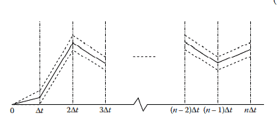
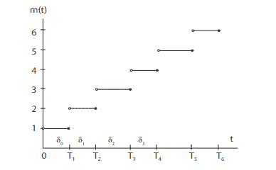
For this, we define a left-continuous function $m(t)$ by $m(t)=j$, while $t \in$ $\left(T_{j-1}, T_{j}\right]$. Succinctly, $m(t)$ represents the index of the next maturity date $.$ Examination of Fig. $5.1$ may help to see the features of $m(t)$.

To show the existence of the LMRW, it is sufficient to give the simplest example for arbitrarily given volatility $\lambda$ and market price of risk $\varphi$. For this, we define a process $\bar{\mu}(t)$ by $\bar{\mu}(t)=\bar{\mu}\left(T_{m(t)}\right)$ such that
$$
\bar{\mu}\left(T_{i}\right)=\frac{1}{\delta_{i-1}} \log \left{1+\delta_{i-1} L_{i-1}\left(T_{i-1}\right)\right}
$$
at each time $T_{i}$. Specifically, $\bar{\mu}(t)$ represents the yield for the shortest maturity bond, with the next maturity $T_{m(t)}$. As a consequence, $\bar{\mu}(t)$ is constant on each period $\left(T_{i-1}, T_{i}\right], i=1, \cdots, n$.

Let $\varphi_{t}$ be an arbitrarily given market price of risk such that $\varphi_{l}$ is an $\mathbf{R}^{d}-$ valued deterministic function with
$$
\int_{0}^{T}\left|\varphi_{t}\right|^{2} d s<\infty $$ Let $\lambda_{i}(t), i=1, \cdots, n$ be deterministic volatilities. We set $\chi_{i}(t)$ as $$ \chi_{i}(t)=\frac{\lambda_{i}(t) \delta_{i} L_{i}(t)}{1+\delta_{i} L_{i}(t)} ; i=1, \cdots, n . $$ Consider the following equation with the initial LIBOR $L_{i}(0)>0$,
$$
\frac{d L_{i}(t)}{L_{i}(t)}=\left{\lambda_{i}(t) \sum_{j=m(t)}^{i} \chi_{j}(t)+\lambda_{i}(t) \varphi_{t}\right} d t+\lambda_{i}(t) d W_{t}
$$
for $i=1, \cdots, n$. It is known that the solution $L_{i}(t)$ exists uniquely and $L_{i}(t)>$ 0 . We assume that bond price processes $B_{i}(t), i=1, \cdots, n$ are Ito processes with initial values $B_{0}(0)=1$ and
$$
B_{i}(0)=\prod_{j=0}^{i-1}\left(1+\delta_{j} L_{j}(0)\right)^{-1}
$$ such that
$$
\frac{d B_{i}(t)}{B_{i}(t)}=\left{\bar{\mu}(t)-\sum_{j=m(t)}^{i-1} \chi_{j}(t) \varphi_{t}\right} d t-\sum_{j=m(t)}^{i-1} \chi_{j}(t) d W_{t} .
$$
Under this setup, we give the following theorem, which shows the existence of the LMRW.

金融代写|利率建模代写Interest Rate Modeling代考|MATH3075

利率建模代考

金融代写|利率建模代写Interest Rate Modeling代考|LIBOR Market Model

LIBOR 市场模型由 Miltersen 等人引入。(1997 年),布雷斯等人。(1997 年;以下称为 BGM)、Musiela 和 Rutkowski(1997 年)和 Jamshidian(1997). 此处列出了此模型的值得注意的点:

  • 该模型具有正 LIBOR。
  • 该模型允许任意确定的波动率结构。
  • 导出caplet和floorlet的价格公式以与对应的布莱克价格一致。
  • 导出了互换期权的近似价格公式。
    由此可见,LIBOR 市场模型在校准方面具有可用性优势,因此被广泛用作衍生品定价的标准模型。作为一个具体的例子,BGM 模型是最知名的 LIBOR 市场模型类型,并且构建在 HJM 框架中。BGM 方法需要一种 LIBOR 波动性的可微性。在实践中不可能满足这种平滑性,因为波动率只能构建为分段连续但不一定平滑的函数。因此,HJM 框架并不严格支持 BGM 模型。有关此问题的更高级研究,请参阅 Yasuoka (2001, 2013b)。

在模型范围的一端,Musiela 和 Rutkowski (1997) 和 Jamshidian (1997) 的方法基于鞅定价理论,没有理论缺陷。然而,他们的模型是在风险中性的衡量标准下构建的,没有参考现实世界的衡量标准。

在本节和下一节中,我们将介绍 Jamshidian (1997) 所描述的 LIBOR 市场模型。因为本书的主题是风险管理,衍生品的定价在这里没有详细讨论。对于更高级的定价处理,建议读者参考 Brigo 和 Mercurio (2007) 或 Gatarek 等人。(2007 年)。

与 HJM 模型的论点类似,当 LIBOR 和债券价格在风险中性度量下表示时,我们称所得系统为风险中性模型。相反,当它们被表示为磷,得到的系统被称为真实世界模型。这些术语的严格定义将在后面给出。

金融代写|利率建模代写Interest Rate Modeling代考|Existence of LIBOR Market Model

LIBOR 模型的存在如下定理所示。
定理 5.2.1 对于任意确定性波动率λ一世(吨),一世=1,⋯,n−1, LIBOR 市场模型存在。

LIBOR 模型可以在多种风险中性措施中的任何一种下构建。应用这一点,我们将在下一节中展示 LIBOR 模型在真实世界度量下的存在,并展示模型在其他度量下的隐含部分5.4和5.5本章的。这种方法被认为是构建 LIBOR 市场模型以供实际使用的最简单方法。因此,我们这里只勾勒出Jamshidian 的LIBOR 市场模型在前向测度下,省略了证明。

让每一个λ一世(吨)是任意确定性函数吨为了一世=1,⋯,n−

  1. 考虑以下等式:
    d大号一世(吨)大号一世(吨)=∑j=一世+1n−1dj大号j(吨)λ一世(吨)λj(吨)1+dj大号jd吨+λ一世(吨)d从吨
    这里,从吨是一个d关于测度的一维布朗运动问(∼ 磷). 通过这种设置,Jamshidian (1997, Corollary 2.1) 给出了以下命题。

命题 5.2.2 方程 (5.4) 承认任意初始条件的唯一正解大号一世(0)>0对于所有我。更远,是一世(吨)=(1+ d一世大号一世(吨))⋯(1+d一世大号n−1(吨))是一个问-鞅。
让乙n(吨)是一个任意的债券价格过程,使得乙n(吨n)=1和

乙n(吨一世)=1∏j=一世n−1(1+dj大号j(吨j))在每一个吨一世. 因此,我们定义乙一世(吨)为了一世<n经过

乙一世(吨)乙n(吨)=∏j=一世n−1(1+dj大号j(吨))
从这些我们可以看出乙一世(吨一世)=1并且关系(5.2)满足所有一世. 根据提案 5.2.2,∏j=一世n−1(1+dj大号j(吨))是每一个 Q-鞅一世. 因此乙一世(吨)/乙n(吨)是所有人的 Q-鞅一世.

沿着这些思路,问是一个乙nnuméraire measure,被称为远期测量。因此,债券市场乙从定理无套利3.2.2

金融代写|利率建模代写Interest Rate Modeling代考|LIBOR Market Model under a Real-world Measure

在与部分相同的设置中5.1和 5.2,我们给出了 LMRW 的定义,并表明模型的存在,遵循 Yasuoka (2013a)。

定义 5.3 债券市场乙被称为大号米R在当满足以下条件时。

  1. LIBOR 流程大号一世,一世=1,⋯,n, 和大号一世(吨)>0, 在真实世界的度量下表示磷这样每个波动率λ一世(吨)和风险的市场价格披吨是确定性的吨.
  2. 债券市场乙无套利;这意味着乙一世(吨)∈乙,一世= 1,⋯,n和国家价格平减指数X吨是正 Ito 过程表示下磷.

为此,我们定义了一个左连续函数米(吨)经过米(吨)=j, 尽管吨∈ (吨j−1,吨j]. 简而言之,米(吨)代表下一个到期日的指数.图的检查5.1可能有助于了解米(吨).

为了证明 LMRW 的存在,给出任意给定波动率的最简单的例子就足够了λ和市场风险价格披. 为此,我们定义了一个流程μ¯(吨)经过μ¯(吨)=μ¯(吨米(吨))这样

\bar{\mu}\left(T_{i}\right)=\frac{1}{\delta_{i-1}} \log \left{1+\delta_{i-1} L_{i-1 }\left(T_{i-1}\right)\right}\bar{\mu}\left(T_{i}\right)=\frac{1}{\delta_{i-1}} \log \left{1+\delta_{i-1} L_{i-1 }\left(T_{i-1}\right)\right}
每次吨一世. 具体来说,μ¯(吨)代表最短期限债券的收益率,下一个到期日吨米(吨). 作为结果,μ¯(吨)在每个时期都是恒定的(吨一世−1,吨一世],一世=1,⋯,n.

让披吨是任意给定的市场风险价格,使得披l是一个Rd−有值的确定性函数

∫0吨|披吨|2ds<∞让λ一世(吨),一世=1,⋯,n是确定性的波动率。我们设置χ一世(吨)作为

χ一世(吨)=λ一世(吨)d一世大号一世(吨)1+d一世大号一世(吨);一世=1,⋯,n.考虑以下具有初始 LIBOR 的等式大号一世(0)>0,

\frac{d L_{i}(t)}{L_{i}(t)}=\left{\lambda_{i}(t) \sum_{j=m(t)}^{i} \chi_{ j}(t)+\lambda_{i}(t) \varphi_{t}\right} d t+\lambda_{i}(t) d W_{t}\frac{d L_{i}(t)}{L_{i}(t)}=\left{\lambda_{i}(t) \sum_{j=m(t)}^{i} \chi_{ j}(t)+\lambda_{i}(t) \varphi_{t}\right} d t+\lambda_{i}(t) d W_{t}
为了一世=1,⋯,n. 据了解,解决方案大号一世(吨)唯一存在并且大号一世(吨)>0 . 我们假设债券价格过程乙一世(吨),一世=1,⋯,n是具有初始值的 Ito 过程乙0(0)=1和

乙一世(0)=∏j=0一世−1(1+dj大号j(0))−1这样

\frac{d B_{i}(t)}{B_{i}(t)}=\left{\bar{\mu}(t)-\sum_{j=m(t)}^{i-1 } \chi_{j}(t) \varphi_{t}\right} d t-\sum_{j=m(t)}^{i-1} \chi_{j}(t) d W_{t} 。\frac{d B_{i}(t)}{B_{i}(t)}=\left{\bar{\mu}(t)-\sum_{j=m(t)}^{i-1 } \chi_{j}(t) \varphi_{t}\right} d t-\sum_{j=m(t)}^{i-1} \chi_{j}(t) d W_{t} 。
在这种设置下,我们给出了以下定理,它表明了 LMRW 的存在。

金融代写|利率建模代写Interest Rate Modeling代考 请认准statistics-lab™

统计代写请认准statistics-lab™. statistics-lab™为您的留学生涯保驾护航。

金融工程代写

金融工程是使用数学技术来解决金融问题。金融工程使用计算机科学、统计学、经济学和应用数学领域的工具和知识来解决当前的金融问题,以及设计新的和创新的金融产品。

非参数统计代写

非参数统计指的是一种统计方法,其中不假设数据来自于由少数参数决定的规定模型;这种模型的例子包括正态分布模型和线性回归模型。

广义线性模型代考

广义线性模型(GLM)归属统计学领域,是一种应用灵活的线性回归模型。该模型允许因变量的偏差分布有除了正态分布之外的其它分布。

术语 广义线性模型(GLM)通常是指给定连续和/或分类预测因素的连续响应变量的常规线性回归模型。它包括多元线性回归,以及方差分析和方差分析(仅含固定效应)。

有限元方法代写

有限元方法(FEM)是一种流行的方法,用于数值解决工程和数学建模中出现的微分方程。典型的问题领域包括结构分析、传热、流体流动、质量运输和电磁势等传统领域。

有限元是一种通用的数值方法,用于解决两个或三个空间变量的偏微分方程(即一些边界值问题)。为了解决一个问题,有限元将一个大系统细分为更小、更简单的部分,称为有限元。这是通过在空间维度上的特定空间离散化来实现的,它是通过构建对象的网格来实现的:用于求解的数值域,它有有限数量的点。边界值问题的有限元方法表述最终导致一个代数方程组。该方法在域上对未知函数进行逼近。[1] 然后将模拟这些有限元的简单方程组合成一个更大的方程系统,以模拟整个问题。然后,有限元通过变化微积分使相关的误差函数最小化来逼近一个解决方案。

tatistics-lab作为专业的留学生服务机构,多年来已为美国、英国、加拿大、澳洲等留学热门地的学生提供专业的学术服务,包括但不限于Essay代写,Assignment代写,Dissertation代写,Report代写,小组作业代写,Proposal代写,Paper代写,Presentation代写,计算机作业代写,论文修改和润色,网课代做,exam代考等等。写作范围涵盖高中,本科,研究生等海外留学全阶段,辐射金融,经济学,会计学,审计学,管理学等全球99%专业科目。写作团队既有专业英语母语作者,也有海外名校硕博留学生,每位写作老师都拥有过硬的语言能力,专业的学科背景和学术写作经验。我们承诺100%原创,100%专业,100%准时,100%满意。

随机分析代写


随机微积分是数学的一个分支,对随机过程进行操作。它允许为随机过程的积分定义一个关于随机过程的一致的积分理论。这个领域是由日本数学家伊藤清在第二次世界大战期间创建并开始的。

时间序列分析代写

随机过程,是依赖于参数的一组随机变量的全体,参数通常是时间。 随机变量是随机现象的数量表现,其时间序列是一组按照时间发生先后顺序进行排列的数据点序列。通常一组时间序列的时间间隔为一恒定值(如1秒,5分钟,12小时,7天,1年),因此时间序列可以作为离散时间数据进行分析处理。研究时间序列数据的意义在于现实中,往往需要研究某个事物其随时间发展变化的规律。这就需要通过研究该事物过去发展的历史记录,以得到其自身发展的规律。

回归分析代写

多元回归分析渐进(Multiple Regression Analysis Asymptotics)属于计量经济学领域,主要是一种数学上的统计分析方法,可以分析复杂情况下各影响因素的数学关系,在自然科学、社会和经济学等多个领域内应用广泛。

MATLAB代写

MATLAB 是一种用于技术计算的高性能语言。它将计算、可视化和编程集成在一个易于使用的环境中,其中问题和解决方案以熟悉的数学符号表示。典型用途包括:数学和计算算法开发建模、仿真和原型制作数据分析、探索和可视化科学和工程图形应用程序开发,包括图形用户界面构建MATLAB 是一个交互式系统,其基本数据元素是一个不需要维度的数组。这使您可以解决许多技术计算问题,尤其是那些具有矩阵和向量公式的问题,而只需用 C 或 Fortran 等标量非交互式语言编写程序所需的时间的一小部分。MATLAB 名称代表矩阵实验室。MATLAB 最初的编写目的是提供对由 LINPACK 和 EISPACK 项目开发的矩阵软件的轻松访问,这两个项目共同代表了矩阵计算软件的最新技术。MATLAB 经过多年的发展,得到了许多用户的投入。在大学环境中,它是数学、工程和科学入门和高级课程的标准教学工具。在工业领域,MATLAB 是高效研究、开发和分析的首选工具。MATLAB 具有一系列称为工具箱的特定于应用程序的解决方案。对于大多数 MATLAB 用户来说非常重要,工具箱允许您学习应用专业技术。工具箱是 MATLAB 函数(M 文件)的综合集合,可扩展 MATLAB 环境以解决特定类别的问题。可用工具箱的领域包括信号处理、控制系统、神经网络、模糊逻辑、小波、仿真等。

R语言代写问卷设计与分析代写
PYTHON代写回归分析与线性模型代写
MATLAB代写方差分析与试验设计代写
STATA代写机器学习/统计学习代写
SPSS代写计量经济学代写
EVIEWS代写时间序列分析代写
EXCEL代写深度学习代写
SQL代写各种数据建模与可视化代写

金融代写|利率建模代写Interest Rate Modeling代考|MTH5520

如果你也在 怎样代写利率建模Interest Rate Modeling这个学科遇到相关的难题,请随时右上角联系我们的24/7代写客服。

利率模型是指一种对利率的运动和演变进行建模的数学方法。它是一种基于市场风险的单因素短利率模型。瓦西克利率模型常用于经济学中,以确定利率在未来的移动方向。

statistics-lab™ 为您的留学生涯保驾护航 在代写利率建模Interest Rate Modeling方面已经树立了自己的口碑, 保证靠谱, 高质且原创的统计Statistics代写服务。我们的专家在代写利率建模Interest Rate Modeling代写方面经验极为丰富,各种代写利率建模Interest Rate Modeling相关的作业也就用不着说。

我们提供的利率建模Interest Rate Modeling及其相关学科的代写,服务范围广, 其中包括但不限于:

  • Statistical Inference 统计推断
  • Statistical Computing 统计计算
  • Advanced Probability Theory 高等概率论
  • Advanced Mathematical Statistics 高等数理统计学
  • (Generalized) Linear Models 广义线性模型
  • Statistical Machine Learning 统计机器学习
  • Longitudinal Data Analysis 纵向数据分析
  • Foundations of Data Science 数据科学基础
金融代写|利率建模代写Interest Rate Modeling代考|MTH5520

金融代写|利率建模代写Interest Rate Modeling代考|The Hull–White Model

In the early days, many stochastic models were introduced to describe the dynamics of the short rate. As examples, see Cox et al. (1985; hereinafter,CIR), Ho and Lee (1986), Hull and White (1990), and Vasicek (1977), among others. A strong point of these models is their parsimoniousness. Additionally, these models are described by affine term structures. For details of affine models, readers are recommended to consult Duffie and Kan (1996), Björk $(2004)$, or Munk (2011).

It is known that the Ho-Lee model and the Hull-White model are special cases of the Gaussian HJM model. The Hull-White model, in particular, is one of the most popular models in many financial institutions. Following along these lines, this section introduces the Hull-White model as a special case of the HJM model.
Short rate process
Let us consider a one-dimensional process of the short rate $r(t)$ represented by
$$
d r(t)=\kappa\left{\theta(t)-r(t)+\frac{\sigma}{\kappa} \varphi_{t}\right} d t+\sigma d W_{t}
$$
where $W_{t}$ is a one-dimensional Brownian motion under the real-world measure $\mathbf{P} ; \kappa$ and $\sigma$ are positive constants; $\theta(t)$ is a positive process; and $\varphi_{t}$ denotes the market price of risk.

It is empirically observed that the volatility of long-term interest rates is less than that of short term rates, reflecting a general phenomenon referred to as mean reversion. To model this feature, the rate at which $r(t)$ reverts to $\theta(t)$ is the speed $\kappa$, called the mean reversion rate.

The savings account $B_{t}=\exp \left{\int_{0}^{t} r(s) d s\right}$ is taken as a numéraire. We set $Z_{t}=\int_{0}^{t} \varphi_{s} d s+W_{t}$. By the Girsanov theorem, there exists a risk-neutral measure $\mathbf{Q}$ equivalent to $\mathbf{P}$ such that $Z_{t}$ is a Brownian motion under $\mathbf{Q}$. From these, the short rate $r(t)$ is represented under $\mathbf{Q}$ as
$$
d r(t)=\kappa(\theta(t)-r(t)) d t+\sigma d Z_{t}
$$
It is known that the price of a zero-coupon bond with maturity $T$ is given by
$$
B(t, T)=\exp {-a(t, T)-b(T-t) r(t)}
$$

金融代写|利率建模代写Interest Rate Modeling代考|VaR Computed in the Real-world

This section studies the reason that the VaR should be computed using a real-world model. For this purpose, the valuation of the VaR depends on the choice of measure. We use the following simple example to illustrate this. For simplicity, we assume a null discount rate in the following argument (i.e. the forward price is equal to the present price).

Suppose a binary bond with expiry at time $T$ and with payoff $X$ at $T$ is given as follows.
$$
\left{\begin{array}{l}
\text { If } L>5 \% \text { at } T, \text { then } X=0 \
\text { If } L \leq 5 \% \text { at } T, \text { then } X=1.01,
\end{array}\right.
$$
where $L$ indicates the 6 -month LIBOR at $T$. Succinctly, the payoff is determined by the level of the 6 -month LIBOR at the expiry date.

The price of this security is computed by using some interest rate model under some risk-neutral measure $\mathbf{Q}$. For the model, we assume the probability distribution of $L$ as
$$
\left{\begin{array}{r}
\mathrm{Q}(L>5 \%)=0.09 \% \
\mathbf{Q}(L \leq 5 \%)=99.01 \%
\end{array}\right.
$$
With this distribution, the arbitrage price of this bond at $t=0$ is calculated by
$$
(1.01 \times 0.9901+0 \times 0.0009) \times 1=1.00
$$ because of the assumption of a null discount rate.
We buy this bond at price $1.00$. Let us valuate the $99 \% \mathrm{VaR}$ of this bond for holding period $T$. We can sell this for the price $1.01$ at time $T$ at a probability of more than $99 \%$. The $99 \% \mathrm{VaR}$ is valuated as the profit of $-0.01(=1.00-1.01)$ under Q.

Next, we assume that historical observation estimates for the 6-month LIBOR are
$$
\left{\begin{array}{l}
\mathbf{P}(L>5 \%)=2 \% \
\mathbf{P}(L \leq 5 \%)=98 \%
\end{array}\right.
$$

金融代写|利率建模代写Interest Rate Modeling代考|Estimation of the Market Price of Risk

In empirical analysis concerning the term structure of interest rates, we are observing historical data under the real-world measure. To give an example, when we use the Hull-White model, the dynamics of the short rate is described from equation $(4.41)$ as
$$
d r(t)=\kappa\left{\theta(t)-r(t)+\frac{\sigma}{\kappa} \varphi_{t}\right} d t+\sigma d W_{t}
$$
To calibrate this model such that this equation explains the historical dynamics of the short rate, we must estimate the parameters $\sigma$ and $\kappa$ and the market price of risk $\varphi_{t}$. In this way, we inevitably estimate $\varphi_{t}$ as part of fitting any interest rate model with the historical dynamics of the interest rates.

Along these lines, there are many studies on estimating the market price of risk in the field of economics. Some papers in this vein are Ahn and Gao (1999), Cheridito et al. (2007), Cochrane and Piazzesi (2010), De Jong (2000), and Duffee (2002). However, there are few papers that explicitly describe the method used in estimating the market price of risk in short rate models. It is even more difficult to find such papers that work with forward rate models.
In this section, we briefly describe three approaches to estimating the market price of risk in short rate models. For a more advanced treatment of this subject, we study theoretical methods for estimating the market price of risk in the forward rate model from Chapter $6 .$

金融代写|利率建模代写Interest Rate Modeling代考|MTH5520

利率建模代考

金融代写|利率建模代写Interest Rate Modeling代考|The Hull–White Model

早期,引入了许多随机模型来描述短期利率的动态。例如,参见 Cox 等人。(1985 年;以下简称 CIR)、Ho 和 Lee(1986 年)、Hull 和 White(1990 年)和 Vasicek(1977 年)等。这些模型的一个优点是它们的简约性。此外,这些模型由仿射术语结构描述。关于仿射模型的详细信息,建议读者参考 Duffie and Kan (1996), Björk(2004),或蒙克(2011 年)。

众所周知,Ho-Lee 模型和 Hull-White 模型是高斯 HJM 模型的特例。赫尔-怀特模型尤其是许多金融机构中最流行的模型之一。沿着这些思路,本节介绍 Hull-White 模型作为 HJM 模型的一个特例。
短利率过程
让我们考虑一个短利率的一维过程r(吨)代表为

d r(t)=\kappa\left{\theta(t)-r(t)+\frac{\sigma}{\kappa} \varphi_{t}\right} d t+\sigma d W_{t}d r(t)=\kappa\left{\theta(t)-r(t)+\frac{\sigma}{\kappa} \varphi_{t}\right} d t+\sigma d W_{t}
在哪里在吨是真实世界测量下的一维布朗运动磷;ķ和σ是正常数;θ(吨)是一个积极的过程;和披吨表示风险的市场价格。

根据经验观察,长期利率的波动性小于短期利率的波动性,反映了一种被称为均值回归的普遍现象。为了对该特征进行建模,速率r(吨)恢复到θ(吨)是速度ķ,称为平均回复率。

储蓄账户B_{t}=\exp \left{\int_{0}^{t} r(s) d s\right}B_{t}=\exp \left{\int_{0}^{t} r(s) d s\right}被视为一个numéraire。我们设置从吨=∫0吨披sds+在吨. 根据 Girsanov 定理,存在风险中性测度问相当于磷这样从吨是下的布朗运动问. 从这些来看,短期利率r(吨)表示在问作为

dr(吨)=ķ(θ(吨)−r(吨))d吨+σd从吨
众所周知,到期零息债券的价格吨是(谁)给的

乙(吨,吨)=经验⁡−一个(吨,吨)−b(吨−吨)r(吨)

金融代写|利率建模代写Interest Rate Modeling代考|VaR Computed in the Real-world

本节研究应使用真实世界模型计算 VaR 的原因。为此,VaR 的估值取决于度量的选择。我们使用下面的简单示例来说明这一点。为简单起见,我们在以下论点中假设折现率为零(即远期价格等于当前价格)。

假设一个二元债券在某个时间到期吨并有回报X在吨给出如下。
$$
\左{

 如果 大号>5% 在 吨, 然后 X=0  如果 大号≤5% 在 吨, 然后 X=1.01,\正确的。
$$
在哪里大号表示 6 个月 LIBOR 在吨. 简而言之,收益取决于到期日的 6 个月 LIBOR 水平。

该证券的价格是通过在某种风险中性措施下使用某种利率模型来计算的问. 对于模型,我们假设概率分布为大号作为
$$
\left{

问(大号>5%)=0.09% 问(大号≤5%)=99.01%\正确的。

在一世吨H吨H一世sd一世s吨r一世b在吨一世○n,吨H和一个rb一世吨r一个G和pr一世C和○F吨H一世sb○nd一个吨$吨=0$一世sC一个lC在l一个吨和db是
(1.01 \times 0.9901+0 \times 0.0009) \times 1=1.00
$$ 因为假设零贴现率。
我们以价格购买该债券1.00. 让我们评估一下99%在一个R本期债券持有期吨. 我们可以卖这个价格1.01有时吨概率大于99%. 这99%在一个R被评估为利润−0.01(=1.00−1.01)Q下。

接下来,我们假设 6 个月 LIBOR 的历史观测估计值为
$$
\left{

磷(大号>5%)=2% 磷(大号≤5%)=98%\正确的。
$$

金融代写|利率建模代写Interest Rate Modeling代考|Estimation of the Market Price of Risk

在利率期限结构的实证分析中,我们是在现实世界的衡量标准下观察历史数据。举个例子,当我们使用 Hull-White 模型时,短期利率的动力学由方程描述(4.41)作为

d r(t)=\kappa\left{\theta(t)-r(t)+\frac{\sigma}{\kappa} \varphi_{t}\right} d t+\sigma d W_{t}d r(t)=\kappa\left{\theta(t)-r(t)+\frac{\sigma}{\kappa} \varphi_{t}\right} d t+\sigma d W_{t}
为了校准这个模型,使这个方程能够解释短期利率的历史动态,我们必须估计参数σ和ķ和风险的市场价格披吨. 这样,我们不可避免地估计披吨作为拟合任何利率模型与利率历史动态的一部分。

沿着这些思路,在经济学领域有许多关于估计风险市场价格的研究。这方面的一些论文是 Ahn 和 Gao (1999),Cheridito 等人。(2007)、Cochrane 和 Piazzesi (2010)、De Jong (2000) 和 Duffee (2002)。然而,很少有论文明确描述在短期利率模型中估计风险市场价格所使用的方法。更难找到适用于远期利率模型的此类论文。
在本节中,我们将简要描述在短期利率模型中估计风险市场价格的三种方法。为了对该主题进行更深入的处理,我们研究了在第 1 章的远期利率模型中估计风险市场价格的理论方法。6.

金融代写|利率建模代写Interest Rate Modeling代考 请认准statistics-lab™

统计代写请认准statistics-lab™. statistics-lab™为您的留学生涯保驾护航。

金融工程代写

金融工程是使用数学技术来解决金融问题。金融工程使用计算机科学、统计学、经济学和应用数学领域的工具和知识来解决当前的金融问题,以及设计新的和创新的金融产品。

非参数统计代写

非参数统计指的是一种统计方法,其中不假设数据来自于由少数参数决定的规定模型;这种模型的例子包括正态分布模型和线性回归模型。

广义线性模型代考

广义线性模型(GLM)归属统计学领域,是一种应用灵活的线性回归模型。该模型允许因变量的偏差分布有除了正态分布之外的其它分布。

术语 广义线性模型(GLM)通常是指给定连续和/或分类预测因素的连续响应变量的常规线性回归模型。它包括多元线性回归,以及方差分析和方差分析(仅含固定效应)。

有限元方法代写

有限元方法(FEM)是一种流行的方法,用于数值解决工程和数学建模中出现的微分方程。典型的问题领域包括结构分析、传热、流体流动、质量运输和电磁势等传统领域。

有限元是一种通用的数值方法,用于解决两个或三个空间变量的偏微分方程(即一些边界值问题)。为了解决一个问题,有限元将一个大系统细分为更小、更简单的部分,称为有限元。这是通过在空间维度上的特定空间离散化来实现的,它是通过构建对象的网格来实现的:用于求解的数值域,它有有限数量的点。边界值问题的有限元方法表述最终导致一个代数方程组。该方法在域上对未知函数进行逼近。[1] 然后将模拟这些有限元的简单方程组合成一个更大的方程系统,以模拟整个问题。然后,有限元通过变化微积分使相关的误差函数最小化来逼近一个解决方案。

tatistics-lab作为专业的留学生服务机构,多年来已为美国、英国、加拿大、澳洲等留学热门地的学生提供专业的学术服务,包括但不限于Essay代写,Assignment代写,Dissertation代写,Report代写,小组作业代写,Proposal代写,Paper代写,Presentation代写,计算机作业代写,论文修改和润色,网课代做,exam代考等等。写作范围涵盖高中,本科,研究生等海外留学全阶段,辐射金融,经济学,会计学,审计学,管理学等全球99%专业科目。写作团队既有专业英语母语作者,也有海外名校硕博留学生,每位写作老师都拥有过硬的语言能力,专业的学科背景和学术写作经验。我们承诺100%原创,100%专业,100%准时,100%满意。

随机分析代写


随机微积分是数学的一个分支,对随机过程进行操作。它允许为随机过程的积分定义一个关于随机过程的一致的积分理论。这个领域是由日本数学家伊藤清在第二次世界大战期间创建并开始的。

时间序列分析代写

随机过程,是依赖于参数的一组随机变量的全体,参数通常是时间。 随机变量是随机现象的数量表现,其时间序列是一组按照时间发生先后顺序进行排列的数据点序列。通常一组时间序列的时间间隔为一恒定值(如1秒,5分钟,12小时,7天,1年),因此时间序列可以作为离散时间数据进行分析处理。研究时间序列数据的意义在于现实中,往往需要研究某个事物其随时间发展变化的规律。这就需要通过研究该事物过去发展的历史记录,以得到其自身发展的规律。

回归分析代写

多元回归分析渐进(Multiple Regression Analysis Asymptotics)属于计量经济学领域,主要是一种数学上的统计分析方法,可以分析复杂情况下各影响因素的数学关系,在自然科学、社会和经济学等多个领域内应用广泛。

MATLAB代写

MATLAB 是一种用于技术计算的高性能语言。它将计算、可视化和编程集成在一个易于使用的环境中,其中问题和解决方案以熟悉的数学符号表示。典型用途包括:数学和计算算法开发建模、仿真和原型制作数据分析、探索和可视化科学和工程图形应用程序开发,包括图形用户界面构建MATLAB 是一个交互式系统,其基本数据元素是一个不需要维度的数组。这使您可以解决许多技术计算问题,尤其是那些具有矩阵和向量公式的问题,而只需用 C 或 Fortran 等标量非交互式语言编写程序所需的时间的一小部分。MATLAB 名称代表矩阵实验室。MATLAB 最初的编写目的是提供对由 LINPACK 和 EISPACK 项目开发的矩阵软件的轻松访问,这两个项目共同代表了矩阵计算软件的最新技术。MATLAB 经过多年的发展,得到了许多用户的投入。在大学环境中,它是数学、工程和科学入门和高级课程的标准教学工具。在工业领域,MATLAB 是高效研究、开发和分析的首选工具。MATLAB 具有一系列称为工具箱的特定于应用程序的解决方案。对于大多数 MATLAB 用户来说非常重要,工具箱允许您学习应用专业技术。工具箱是 MATLAB 函数(M 文件)的综合集合,可扩展 MATLAB 环境以解决特定类别的问题。可用工具箱的领域包括信号处理、控制系统、神经网络、模糊逻辑、小波、仿真等。

R语言代写问卷设计与分析代写
PYTHON代写回归分析与线性模型代写
MATLAB代写方差分析与试验设计代写
STATA代写机器学习/统计学习代写
SPSS代写计量经济学代写
EVIEWS代写时间序列分析代写
EXCEL代写深度学习代写
SQL代写各种数据建模与可视化代写

金融代写|利率建模代写Interest Rate Modeling代考|MATH5985

如果你也在 怎样代写利率建模Interest Rate Modeling这个学科遇到相关的难题,请随时右上角联系我们的24/7代写客服。

利率模型是指一种对利率的运动和演变进行建模的数学方法。它是一种基于市场风险的单因素短利率模型。瓦西克利率模型常用于经济学中,以确定利率在未来的移动方向。

statistics-lab™ 为您的留学生涯保驾护航 在代写利率建模Interest Rate Modeling方面已经树立了自己的口碑, 保证靠谱, 高质且原创的统计Statistics代写服务。我们的专家在代写利率建模Interest Rate Modeling代写方面经验极为丰富,各种代写利率建模Interest Rate Modeling相关的作业也就用不着说。

我们提供的利率建模Interest Rate Modeling及其相关学科的代写,服务范围广, 其中包括但不限于:

  • Statistical Inference 统计推断
  • Statistical Computing 统计计算
  • Advanced Probability Theory 高等概率论
  • Advanced Mathematical Statistics 高等数理统计学
  • (Generalized) Linear Models 广义线性模型
  • Statistical Machine Learning 统计机器学习
  • Longitudinal Data Analysis 纵向数据分析
  • Foundations of Data Science 数据科学基础
金融代写|利率建模代写Interest Rate Modeling代考|MATH5985

金融代写|利率建模代写Interest Rate Modeling代考|Heath-Jarrow-Morton Framework

We introduced a bond market $\mathcal{B}$ in Chapter 3 that did not admit a term structure of interest rates. If, instead, we assume a term structure in the bond market, it becomes possible to relate the bond price to the interest rate. We represent the dynamics of bond price by a stochastic process and use this to specify the corresponding interest rates. Such a system is referred to as a term structure model of interest rates (or put simply, an interest rate model).
A model specified by the dynamics of a short rate is referred to as a short rate model. A model specified by the dynamics of forward rates is referred to as a forward rate model. For management of interest rate risk, it is better to suppose various types of changes in the yield curve, and specifically to suppose changes in the forward rates. Because of this, the forward rate model is more useful in risk management than the short rate model is.

This section briefly introduces the HJM model, which is the most general forward rate model. For additional details, readers are recommended to consult Cairns (2004), Munk (2011), or Shreve (2004), among others. For details on calibration, readers are recommended to consult Wu (2009).
Forward rate process
Let $\left(\Omega, \mathcal{F}{t \in[0, \tau]}, \mathbf{P}\right)$ be a filtered probability space, where $\mathcal{F}{t \in[0, \tau]}$ is the augmented filtration and $\mathbf{P}$ denotes the real-world measure. The instantaneous forward rate with maturity $T$ observed at time $t$ is denoted by $f(t, T)$. When the usage is unambiguous, $f(t, T)$ will be called the forward rate. Typically $f(0, T)$ represents an initial forward rate.

We assume that the dynamics of $f(t, T)$ on $\left(\Omega, \mathcal{F}{t \in[0, \tau]}, \mathbf{P}\right)$ is represented by $$ d f(t, T)=\alpha(t, T) d t+\sigma(t, T) d W{t},
$$
where $W_{t}=\left(W_{t}^{1}, \cdots, W_{t}^{d}\right)^{T}$ is a $d$-dimensional P-Brownian motion, and $\alpha(t, T)$ and $\sigma(t, T)$ are predictable processes satisfying some technical conditions. Here, $\sigma(t, T)=\left(\sigma^{1}(t, T), \cdots, \sigma^{d}(t, T)\right)^{T}$ is a $d$-dimensional process. The second term, $\sigma(t, T) d W_{t}$ denotes the inner product of $\sigma(t, T)$ and $d W_{t}$ in $\mathbf{R}^{d}$, specifically
$$
\sigma(t, T) d W_{t}=\sum_{l=1}^{d} \sigma^{l}(t, T) d W_{t}^{l} .
$$

金融代写|利率建模代写Interest Rate Modeling代考|Arbitrage Pricing and Market Price of Risk

This section briefly studies some fundamental subjects in the HJM model, specifically, forward rate process, arbitrage pricing, the market price of risk, and state price deflator.
Forward rate process
Here let us represent the forward rate process under the risk-neutral measure Q. Differentiating equation (4.9) with respect to $T$, we have
$$
-\alpha(s, T)-\sigma(s, T) \int_{s}^{T} \sigma(s, u) d u=\frac{\partial b(s, T)}{\partial T} .
$$
From equations (4.10) and (4.12), it follows that
$$
\begin{aligned}
-\alpha(s, T)-\sigma(s, T) \int_{s}^{T} \sigma(s, u) d u &=\frac{\partial v(s, T)}{\partial T} \varphi_{t} \
&=-\sigma(s, T) \varphi_{t}
\end{aligned}
$$
Substituting the above into equation (4.1), we obtain
$$
d f(t, T)={-\sigma(t, T) v(t, T)+\sigma(t, T) \varphi(t)} d t+\sigma(t, T) d W_{t}
$$
Recall the Q-Brownian motion $Z_{t}=\int_{0}^{t} \varphi_{s} d s+W_{t}$. Substituting this into the above, we have
$$
d f(t, T)=-\sigma(t, T) v(t, T) d t+\sigma(t, T) d Z_{t}
$$
where the drift under $\mathbf{Q}$ is completely determined by the volatility $\sigma(t, T)$. This form is the well-known forward rate process in the HJM model. For pricing interest rate derivatives, the dynamics of the forward rates are typically simulated by equation (4.18), and the bond pricing is performed by using this form. This method is essentially the same as used with short rate models.

金融代写|利率建模代写Interest Rate Modeling代考|Volatility and Principal Components

This section introduces a method for constructing the volatility in the H.JM model. There are two major approaches to do so. One is a market approach; the other is a historical approach.

In the market approach, the volatility is estimated such that the model implies option prices consistent with their market prices. In the historical approach, the volatility is constructed to represent a historical dynamics of an interest rate, for example, the short rate or the forward rate. Experimentally, these two approaches result in quite different volatility structures.

When we calibrate the model for derivatives pricing, the market approach should be employed. In this, it is understood that historical volatility cannot explain market prices because the option prices are determined mostly by traders’ forecasts for the future market rather than by historical volatility. Therefore, adopting a historical approach will result in a model that misprices major derivatives. Such a model is not valid for derivatives trading.

However, when we intend to calibrate a model for interest-risk-management, the historical approach is recommended, rather than the market approach. In the historical approach, principal component analysis (PCA) is a standard technique for reducing the dimensionality of the model. PCA will be repeatedly used in this book, and we introduce the construction of volatility by applying PCA. The fundamentals of PCA and the relevant linear algebra are given in Appendix B.

金融代写|利率建模代写Interest Rate Modeling代考|MATH5985

利率建模代考

金融代写|利率建模代写Interest Rate Modeling代考|Heath-Jarrow-Morton Framework

我们引入了债券市场乙在第 3 章中没有承认利率的期限结构。相反,如果我们假设债券市场的期限结构,则可以将债券价格与利率联系起来。我们用随机过程来表示债券价格的动态,并用它来指定相应的利率。这样的系统被称为利率期限结构模型(或简单地说,利率模型)。
由短期利率动态指定的模型称为短期利率模型。由远期利率动态指定的模型称为远期利率模型。对于利率风险的管理,最好假设收益率曲线的各种变化,特别是假设远期利率的变化。因此,远期利率模型在风险管理中比短期利率模型更有用。

本节简单介绍 HJM 模型,它是最通用的远期利率模型。有关更多详细信息,建议读者查阅 Cairns (2004)、Munk (2011) 或 Shreve (2004) 等。有关校准的详细信息,建议读者参考 Wu (2009)。
远期汇率过程
Let(Ω,F吨∈[0,τ],磷)是一个过滤的概率空间,其中F吨∈[0,τ]是增强过滤和磷表示真实世界的度量。到期的瞬时远期利率吨当时观察到吨表示为F(吨,吨). 用法明确时,F(吨,吨)将被称为远期利率。通常F(0,吨)表示初始远期利率。

我们假设动态F(吨,吨)上(Ω,F吨∈[0,τ],磷)表示为

dF(吨,吨)=一个(吨,吨)d吨+σ(吨,吨)d在吨,
在哪里在吨=(在吨1,⋯,在吨d)吨是一个d维P-布朗运动,和一个(吨,吨)和σ(吨,吨)是满足某些技术条件的可预测过程。这里,σ(吨,吨)=(σ1(吨,吨),⋯,σd(吨,吨))吨是一个d维过程。第二学期,σ(吨,吨)d在吨表示的内积σ(吨,吨)和d在吨在Rd, 具体来说

σ(吨,吨)d在吨=∑l=1dσl(吨,吨)d在吨l.

金融代写|利率建模代写Interest Rate Modeling代考|Arbitrage Pricing and Market Price of Risk

本节简要研究 HJM 模型中的一些基本主题,特别是远期利率过程、套利定价、风险的市场价格和国家价格平减指数。
远期利率过程
这里让我们表示在风险中性度量 Q 下的远期利率过程。微分方程(4.9)关于吨, 我们有

−一个(s,吨)−σ(s,吨)∫s吨σ(s,在)d在=∂b(s,吨)∂吨.
从方程 (4.10) 和 (4.12) 可以得出

−一个(s,吨)−σ(s,吨)∫s吨σ(s,在)d在=∂在(s,吨)∂吨披吨 =−σ(s,吨)披吨
将上述代入方程(4.1),我们得到

dF(吨,吨)=−σ(吨,吨)在(吨,吨)+σ(吨,吨)披(吨)d吨+σ(吨,吨)d在吨
回想一下 Q-布朗运动从吨=∫0吨披sds+在吨. 将其代入上述,我们有

dF(吨,吨)=−σ(吨,吨)在(吨,吨)d吨+σ(吨,吨)d从吨
漂流在哪里问完全由波动率决定σ(吨,吨). 这种形式是 HJM 模型中众所周知的远期利率过程。对于利率衍生品的定价,远期利率的动态通常由方程(4.18)模拟,债券定价采用这种形式。这种方法本质上与用于短期模型的方法相同。

金融代写|利率建模代写Interest Rate Modeling代考|Volatility and Principal Components

本节介绍一种在 H.JM 模型中构建波动率的方法。有两种主要方法可以做到这一点。一是市场方法;另一种是历史方法。

在市场方法中,对波动率的估计使得模型暗示期权价格与其市场价格一致。在历史方法中,波动率被构建为代表利率的历史动态,例如短期利率或远期利率。在实验上,这两种方法导致了完全不同的波动率结构。

当我们校准衍生品定价模型时,应采用市场方法。在此,可以理解的是,历史波动率并不能解释市场价格,因为期权价格主要取决于交易者对未来市场的预测,而不是历史波动率。因此,采用历史方法将导致模型对主要衍生品进行错误定价。这种模型不适用于衍生品交易。

然而,当我们打算校准一个利率风险管理模型时,建议使用历史方法,而不是市场方法。在历史方法中,主成分分析 (PCA) 是降低模型维数的标准技术。本书将重复使用 PCA,我们将通过应用 PCA 来介绍波动率的构建。PCA 的基础知识和相关的线性代数在附录 B 中给出。

金融代写|利率建模代写Interest Rate Modeling代考 请认准statistics-lab™

统计代写请认准statistics-lab™. statistics-lab™为您的留学生涯保驾护航。

金融工程代写

金融工程是使用数学技术来解决金融问题。金融工程使用计算机科学、统计学、经济学和应用数学领域的工具和知识来解决当前的金融问题,以及设计新的和创新的金融产品。

非参数统计代写

非参数统计指的是一种统计方法,其中不假设数据来自于由少数参数决定的规定模型;这种模型的例子包括正态分布模型和线性回归模型。

广义线性模型代考

广义线性模型(GLM)归属统计学领域,是一种应用灵活的线性回归模型。该模型允许因变量的偏差分布有除了正态分布之外的其它分布。

术语 广义线性模型(GLM)通常是指给定连续和/或分类预测因素的连续响应变量的常规线性回归模型。它包括多元线性回归,以及方差分析和方差分析(仅含固定效应)。

有限元方法代写

有限元方法(FEM)是一种流行的方法,用于数值解决工程和数学建模中出现的微分方程。典型的问题领域包括结构分析、传热、流体流动、质量运输和电磁势等传统领域。

有限元是一种通用的数值方法,用于解决两个或三个空间变量的偏微分方程(即一些边界值问题)。为了解决一个问题,有限元将一个大系统细分为更小、更简单的部分,称为有限元。这是通过在空间维度上的特定空间离散化来实现的,它是通过构建对象的网格来实现的:用于求解的数值域,它有有限数量的点。边界值问题的有限元方法表述最终导致一个代数方程组。该方法在域上对未知函数进行逼近。[1] 然后将模拟这些有限元的简单方程组合成一个更大的方程系统,以模拟整个问题。然后,有限元通过变化微积分使相关的误差函数最小化来逼近一个解决方案。

tatistics-lab作为专业的留学生服务机构,多年来已为美国、英国、加拿大、澳洲等留学热门地的学生提供专业的学术服务,包括但不限于Essay代写,Assignment代写,Dissertation代写,Report代写,小组作业代写,Proposal代写,Paper代写,Presentation代写,计算机作业代写,论文修改和润色,网课代做,exam代考等等。写作范围涵盖高中,本科,研究生等海外留学全阶段,辐射金融,经济学,会计学,审计学,管理学等全球99%专业科目。写作团队既有专业英语母语作者,也有海外名校硕博留学生,每位写作老师都拥有过硬的语言能力,专业的学科背景和学术写作经验。我们承诺100%原创,100%专业,100%准时,100%满意。

随机分析代写


随机微积分是数学的一个分支,对随机过程进行操作。它允许为随机过程的积分定义一个关于随机过程的一致的积分理论。这个领域是由日本数学家伊藤清在第二次世界大战期间创建并开始的。

时间序列分析代写

随机过程,是依赖于参数的一组随机变量的全体,参数通常是时间。 随机变量是随机现象的数量表现,其时间序列是一组按照时间发生先后顺序进行排列的数据点序列。通常一组时间序列的时间间隔为一恒定值(如1秒,5分钟,12小时,7天,1年),因此时间序列可以作为离散时间数据进行分析处理。研究时间序列数据的意义在于现实中,往往需要研究某个事物其随时间发展变化的规律。这就需要通过研究该事物过去发展的历史记录,以得到其自身发展的规律。

回归分析代写

多元回归分析渐进(Multiple Regression Analysis Asymptotics)属于计量经济学领域,主要是一种数学上的统计分析方法,可以分析复杂情况下各影响因素的数学关系,在自然科学、社会和经济学等多个领域内应用广泛。

MATLAB代写

MATLAB 是一种用于技术计算的高性能语言。它将计算、可视化和编程集成在一个易于使用的环境中,其中问题和解决方案以熟悉的数学符号表示。典型用途包括:数学和计算算法开发建模、仿真和原型制作数据分析、探索和可视化科学和工程图形应用程序开发,包括图形用户界面构建MATLAB 是一个交互式系统,其基本数据元素是一个不需要维度的数组。这使您可以解决许多技术计算问题,尤其是那些具有矩阵和向量公式的问题,而只需用 C 或 Fortran 等标量非交互式语言编写程序所需的时间的一小部分。MATLAB 名称代表矩阵实验室。MATLAB 最初的编写目的是提供对由 LINPACK 和 EISPACK 项目开发的矩阵软件的轻松访问,这两个项目共同代表了矩阵计算软件的最新技术。MATLAB 经过多年的发展,得到了许多用户的投入。在大学环境中,它是数学、工程和科学入门和高级课程的标准教学工具。在工业领域,MATLAB 是高效研究、开发和分析的首选工具。MATLAB 具有一系列称为工具箱的特定于应用程序的解决方案。对于大多数 MATLAB 用户来说非常重要,工具箱允许您学习应用专业技术。工具箱是 MATLAB 函数(M 文件)的综合集合,可扩展 MATLAB 环境以解决特定类别的问题。可用工具箱的领域包括信号处理、控制系统、神经网络、模糊逻辑、小波、仿真等。

R语言代写问卷设计与分析代写
PYTHON代写回归分析与线性模型代写
MATLAB代写方差分析与试验设计代写
STATA代写机器学习/统计学习代写
SPSS代写计量经济学代写
EVIEWS代写时间序列分析代写
EXCEL代写深度学习代写
SQL代写各种数据建模与可视化代写