如果你也在 怎样代写数值方法numerical methods这个学科遇到相关的难题，请随时右上角联系我们的24/7代写客服。

如果所有导数的近似值（有限差分、有限元、有限体积等）在步长（Δt、Δx等）趋于零时都趋于精确值，则称该数值方法为一致的。如果误差不随时间（或迭代）增长，则表示数值方法是稳定的（如IVPs）。

statistics-lab™ 为您的留学生涯保驾护航 在代写数值方法numerical methods方面已经树立了自己的口碑, 保证靠谱, 高质且原创的统计Statistics代写服务。我们的专家在代写数值方法numerical methods代写方面经验极为丰富，各种代写数值方法numerical methods相关的作业也就用不着说。

我们提供的数值方法numerical methods及其相关学科的代写，服务范围广, 其中包括但不限于:

• Statistical Inference 统计推断
• Statistical Computing 统计计算
• Advanced Probability Theory 高等概率论
• Advanced Mathematical Statistics 高等数理统计学
• (Generalized) Linear Models 广义线性模型
• Statistical Machine Learning 统计机器学习
• Longitudinal Data Analysis 纵向数据分析
• Foundations of Data Science 数据科学基础

数学代写|数值方法作业代写numerical methods代考|Qualitative Properties of the Solution and Maximum Principle

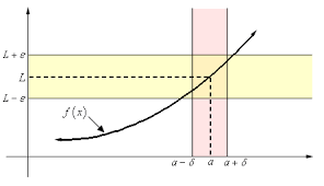
Before we introduce difference schemes for (2.1), we discuss a number of results that allow us to describe how the solution $u$ behaves. First, we wish to conclude that if the initial value $A$ and inhomogeneous term $f(t)$ are positive, then the solution $u(t)$ should also be positive for any value $t$ in $[0, T]$. This so-called positivity or monotonicity result should be reflected in our difference schemes (not all schemes possess this property). Second, we wish to know how the solution $u(t)$ grows or decreases as a function of time. The following two results deal with these issues.

Lemma 2.1 (Positivity). Let the operator $L$ be defined in Equation (2.1), and let $w$ be a well-behaved function satisfying the inequalities:
$$
\begin{aligned}
&L w(t) \geq 0 \forall t \in[0, T] \
&w(0) \geq 0
\end{aligned}
$$

Then the following result holds true:
$$
w(t) \geq 0 \forall t \in[0, T] .
$$
Roughly speaking, this lemma states that you cannot get a negative solution from positive input.
You can verify it by examining Equation (2.2) because all terms are positive. The following result gives bounds on the growth of $u(t)$.
Theorem 2.1 Let $u(t)$ be the solution of Equation (2.1). Then:
$$
|u(t)| \leq \frac{N}{\alpha}+|A| \forall t \in[0, T]
$$
where
$$
|f(t)| \leq N \forall t \in[0, T] .
$$
This result states that the value of the solution is bounded by the input data. In other words, it is a well-posed problem.

We wish to replicate these properties in our difference schemes for Equation (2.1). For completeness, we show the steps to be executed in order to produce the result in Equation (2.2).
$$
\text { Let } I(t)=\exp \left(\int_{0}^{t} a(s) d s\right), \quad I^{-1}(t)=\exp \left(-\int_{0}^{t} a(s) d s\right) \text {. }
$$
Then from Equation (2.1) we see:
$$
I(t)\left(\frac{d u}{d t}+a u\right)=I(t) f(t)
$$
or:
$$
\frac{d}{d t}(I(t) u)=I(t) f(t) .
$$
Integrating this equation between $t=0$ and $t=\xi$ gives:
$$
\begin{aligned}
&\left.\int_{0}^{\xi} \frac{d}{d t}(I(t) u) d t=\int_{0}^{\xi} I(t) f(t) d t \text { (and using the fact that } I(0)=1\right) \
&I(\xi) u(\xi)=u(0)+\int_{0}^{\xi} I(t) f(t) d t \
&u(\xi)=u(0) I^{-1}(\xi)+I^{-1}(\xi) \int_{0}^{\xi} I(t) f(t) d t \
&=\exp \left(-\int_{0}^{\xi} a(s) d s\right) u(0)+\exp \left(-\int_{0}^{\xi} a(s) d s\right) \int_{0}^{\xi} I(t) f(t) d t
\end{aligned}
$$

数学代写|数值方法作业代写numerical methods代考|Rationale and Generalisations

The IVP Equation (2.1) is a model for all the linear time-dependent differential equations that we encounter in this book. We no longer think in terms of scalar problems in which the functions in Equation (2.1) are scalar-valued, but we can view an ODE at different levels of abstraction. To this end, we focus on the generic homogeneous $O D E$ with solution $u(t)$ :
$$
\frac{d u}{d t}=A u, t>0 .
$$
This equation subsumes several special cases:

1. The variable $A$ is a square matrix, and then Equation (2.4) represents a system of ODEs. This is a very important area of research having many applications in science, engineering, and finance.
2. The variable $A$ is an ordinary or partial differential operator, and then Equation (2.4) represents an ODE in a Hilbert or Banach space.
3. The variable $A$ is a tridiagonal or block tridiagonal matrix that originates from a semi-discretisation in space of a time-dependent partial differential equation (PDE) using the Method of Lines (MOL) as discussed in Chapter $20 .$
4. The formal solution of $(2.4)$ is:
   $$
   u(t)=u(0) e^{A t}, \quad t>0
   $$
   In other words, we express the solution in terms of the exponential function of a matrix or of a differential operator. In the former case, there are many ways to compute the exponential of a matrix (see Moler and Van Loan (2003)).
5. The solution of Equation (2.4) can be simplified by matrix or operator splitting of the operator $A$ :
   $$
   \begin{aligned}
   &A=A_{1}+A_{2} \
   &\frac{d u}{d t}=A_{1} u \
   &\frac{d u}{d t}=A_{2} u .
   \end{aligned}
   $$
   For example, we can split a matrix $A$ into two simpler matrices, or we can split an operator $A$ into its convection and diffusion components. In other words, we solve Equation (2.4) as a sequence of simpler problems in (2.6). These topics will be discussed in Chapters 18,22 , and 23 .
6. The initial value problem (2.1) was originally used as a model test of finite difference methods in (Dahlquist (1956)). The resulting results and insights are helpful when dealing more complex IVPs.

数学代写|数值方法作业代写numerical methods代考|DISCRETISATION OF INITIAL VALUE PROBLEMS: FUNDAMENTALS

We now discuss finding an approximate solution to Equation (2.1) using the finite difference method. We introduce several popular schemes as well as defining standardised notation.

The interval or range where the solution of Equation $(2.1)$ is defined is $[0, T]$. When approximating the solution using finite difference equations, we use a discrete set of points in $[0, T]$ where the discrete solution will be calculated. To this end, we divide $[0, T]$ into $N$ equal intervals of length $k$, where $k$ is a positive number called the step size. (We also use the symbol $\Delta t$ to denote the step size in many cases.) We number these discrete points as shown in Figure 2.1. In general all coefficients and discrete functions will be defined at these mesh points only. We adopt the following notation:
$$
\begin{aligned}
&a^{n}=a\left(t_{n}\right), f^{n}=f\left(t_{n}\right) \
&a^{n, \theta}=a\left(\theta t_{n}+(1-\theta) t_{n+1}\right), 0 \leq \theta \leq 1,0 \leq n \leq N-1 \
&u^{n, \theta}=\theta u^{n}+(1-\theta) u^{n+1}, 0 \leq n \leq N-1 \text { (function to be calculated). }
\end{aligned}
$$
Not only do we have to approximate functions at mesh points, but we also have to come up with a scheme to approximate the derivative appearing in Equation (2.1). There are several possibilities, and they are based on divided differences. For example, the following divided differences approximate the first derivative of $u$ at the mesh point $t_{n}=n * k$;
$$
\left.\begin{array}{l}
D_{+} u^{n} \equiv \frac{u^{n+1}-u^{n}}{k} \
D_{-} u^{n} \equiv \frac{u^{n}-u^{n-1}}{k} \
D_{0} u^{n} \equiv \frac{u^{n+1}-u^{n-1}}{2 k}
\end{array}\right}
$$
The first two divided differences are called one-sided differences and give first-order accuracy to the derivative, while the last divided difference is called a centred approximation to the derivative. In fact, by using a Taylor’s expansion (assuming sufficient

smoothness of $u$ ), we can prove the following:
$$
\left{\begin{array}{l}
\left|D_{\pm} u\left(t_{n}\right)-u^{\prime}\left(t_{n}\right)\right| \leq M k, n=0,1, \ldots \
\left|D_{0} u\left(t_{n}\right)-u^{\prime}\left(t_{n}\right)\right| \leq M k^{2}, n=0,1, \ldots
\end{array}\right.
$$
Note that the first two approximations use two consecutive mesh points while the last formula uses three consecutive mesh points.

We now decide on how to approximate Equation (2.1) using finite differences. To this end, we need to introduce two new concepts:

• One-step and multistep methods
• Explicit and implicit schemes.
  A one-step method is a finite difference scheme that calculates the solution at time-level $n+1$ in terms of the solution at time-level $n$. No information at levels $n-1$, $n-2$, or previous levels is needed in order to calculate the solution at level $n+1$. A multistep method, on the other hand, is a difference scheme where the solution at level $n+1$ is determined by values at levels $n, n-1$ and possibly previous time levels. Multistep methods are more complicated than one-step methods, and we concentrate solely on the latter methods in this book.

An explicit difference scheme is one where the solution at time $n+1$ can be calculated from the information at level $n$ directly. No extra arithmetic is needed: for example, using division or matrix inversion. An implicit finite difference scheme is one in which the terms involving the approximate solution at level $n+1$ are grouped together and only then can the solution at this level be found. Obviously, implicit methods are more difficult to program than explicit methods because we must solve a system of equations at each time step.

数值方法代写

数学代写|数值方法作业代写numerical methods代考|Qualitative Properties of the Solution and Maximum Principle

在我们介绍 (2.1) 的差分方案之前，我们讨论了一些结果，这些结果使我们能够描述解决方案在行为。首先，我们希望得出结论，如果初始值一种和不齐项F(吨)为正，则解在(吨)对于任何值也应该是正数吨在[0,吨]. 这种所谓的正性或单调性结果应该反映在我们的差分方案中（并非所有方案都具有此属性）。二、想知道怎么解决在(吨)随时间增加或减少。以下两个结果处理了这些问题。

引理 2.1（积极性）。让运营商大号在等式（2.1）中定义，并让在是满足不等式的表现良好的函数：
大号在(吨)≥0∀吨∈[0,吨] 在(0)≥0

那么以下结果成立：
在(吨)≥0∀吨∈[0,吨].
粗略地说，这个引理表明你不能从正输入中得到负解。
您可以通过检查等式 (2.2) 来验证它，因为所有项都是正数。以下结果给出了增长的界限在(吨).
定理 2.1 让在(吨)是方程（2.1）的解。然后：
|在(吨)|≤ñ一种+|一种|∀吨∈[0,吨]
在哪里
|F(吨)|≤ñ∀吨∈[0,吨].
该结果表明解决方案的值受输入数据的限制。换句话说，这是一个适定问题。

我们希望在方程（2.1）的差分方案中复制这些属性。为了完整起见，我们展示了为产生等式 (2.2) 中的结果而要执行的步骤。
 让 一世(吨)=经验⁡(∫0吨一种(s)ds),一世−1(吨)=经验⁡(−∫0吨一种(s)ds). 
然后从方程（2.1）我们看到：
一世(吨)(d在d吨+一种在)=一世(吨)F(吨)
或者：
dd吨(一世(吨)在)=一世(吨)F(吨).
积分之间的这个方程吨=0和吨=X给出：
∫0Xdd吨(一世(吨)在)d吨=∫0X一世(吨)F(吨)d吨 （并使用以下事实 一世(0)=1) 一世(X)在(X)=在(0)+∫0X一世(吨)F(吨)d吨 在(X)=在(0)一世−1(X)+一世−1(X)∫0X一世(吨)F(吨)d吨 =经验⁡(−∫0X一种(s)ds)在(0)+经验⁡(−∫0X一种(s)ds)∫0X一世(吨)F(吨)d吨

数学代写|数值方法作业代写numerical methods代考|Rationale and Generalisations

IVP 方程（2.1）是我们在本书中遇到的所有线性时间相关微分方程的模型。我们不再考虑方程 (2.1) 中的函数是标量值的标量问题，但我们可以在不同抽象级别上查看 ODE。为此，我们专注于泛型同构这D和有溶液在(吨) :
d在d吨=一种在,吨>0.
这个等式包含了几种特殊情况：

1. 变量一种是一个方阵，则方程 (2.4) 表示一个 ODE 系统。这是一个非常重要的研究领域，在科学、工程和金融领域有许多应用。
2. 变量一种是普通或偏微分算子，则方程 (2.4) 表示希尔伯特或巴纳赫空间中的 ODE。
3. 变量一种是一个三对角矩阵或块三对角矩阵，它源自使用线法 (MOL) 对时间相关偏微分方程 (PDE) 进行空间半离散化，如第 1 章所述20.
4. 的正式解决方案(2.4)是：
   在(吨)=在(0)和一种吨,吨>0
   换句话说，我们用矩阵或微分算子的指数函数来表达解。在前一种情况下，有很多方法可以计算矩阵的指数（参见 Moler 和 Van Loan (2003)）。
5. 方程（2.4）的解可以通过矩阵或算子的算子拆分来简化一种 :
   一种=一种1+一种2 d在d吨=一种1在 d在d吨=一种2在.
   例如，我们可以拆分一个矩阵一种分成两个更简单的矩阵，或者我们可以拆分一个运算符一种分为对流和扩散成分。换句话说，我们将方程（2.4）求解为（2.6）中的一系列更简单的问题。这些主题将在第 18、22 和 23 章中讨论。
6. 初始值问题 (2.1) 最初在 (Dahlquist (1956)) 中用作有限差分方法的模型检验。在处理更复杂的 IVP 时，得到的结果和见解很有帮助。

数学代写|数值方法作业代写numerical methods代考|DISCRETISATION OF INITIAL VALUE PROBLEMS: FUNDAMENTALS

我们现在讨论使用有限差分法寻找方程（2.1）的近似解。我们介绍了几种流行的方案以及定义标准化符号。

方程解的区间或范围(2.1)被定义为[0,吨]. 当使用有限差分方程逼近解时，我们使用一组离散的点[0,吨]将计算离散解的位置。为此，我们分[0,吨]进入ñ等长间隔ķ， 在哪里ķ是一个正数，称为步长。（我们也使用符号Δ吨在许多情况下表示步长。）我们对这些离散点进行编号，如图 2.1 所示。一般来说，所有系数和离散函数都将仅在这些网格点处定义。我们采用以下符号：
一种n=一种(吨n),Fn=F(吨n) 一种n,θ=一种(θ吨n+(1−θ)吨n+1),0≤θ≤1,0≤n≤ñ−1 在n,θ=θ在n+(1−θ)在n+1,0≤n≤ñ−1 （要计算的函数）。 
我们不仅要逼近网格点处的函数，而且我们还必须提出一个方案来逼近方程（2.1）中出现的导数。有几种可能性，它们是基于分歧的。例如，以下划分的差异近似于的一阶导数在在网格点吨n=n∗ķ;
\left.\begin{array}{l} D_{+} u^{n} \equiv \frac{u^{n+1}-u^{n}}{k} \ D_{-} u^{ n} \equiv \frac{u^{n}-u^{n-1}}{k} \ D_{0} u^{n} \equiv \frac{u^{n+1}-u^{ n-1}}{2 k} \end{数组}\right}\left.\begin{array}{l} D_{+} u^{n} \equiv \frac{u^{n+1}-u^{n}}{k} \ D_{-} u^{ n} \equiv \frac{u^{n}-u^{n-1}}{k} \ D_{0} u^{n} \equiv \frac{u^{n+1}-u^{ n-1}}{2 k} \end{数组}\right}
前两个划分的差异称为单边差分，并为导数提供一阶精度，而最后一个划分的差异称为导数的中心近似。事实上，通过使用泰勒展开式（假设足够

光滑度在)，我们可以证明如下：
$$
\left{|D±在(吨n)−在′(吨n)|≤米ķ,n=0,1,… |D0在(吨n)−在′(吨n)|≤米ķ2,n=0,1,…\对。
$$
请注意，前两个近似使用两个连续的网格点，而最后一个公式使用三个连续的网格点。

我们现在决定如何使用有限差分逼近方程（2.1）。为此，我们需要引入两个新概念：

• 一步法和多步法
• 显式和隐式方案。
  一步法是一种有限差分方案，它在时间级计算解n+1就时间层面的解决方案而言n. 没有级别信息n−1, n−2，或者需要以前的级别才能计算级别的解决方案n+1. 另一方面，多步法是一种差分方案，其中水平的解决方案n+1由级别的值决定n,n−1可能还有以前的时间水平。多步法比一步法更复杂，本书只关注后一种方法。

显式差分方案是一种在时间上的解决方案n+1可以从级别的信息中计算出来n直接地。不需要额外的算术：例如，使用除法或矩阵求逆。隐式有限差分格式是其中涉及级别近似解的项n+1组合在一起，然后才能找到该级别的解决方案。显然，隐式方法比显式方法更难编程，因为我们必须在每个时间步求解方程组。

数值方法代写

数学代写|数值方法作业代写numerical methods代考|Lipschitz Continuous Functions

我们现在检查将一个度量空间映射到另一个度量空间的函数。特别是，我们讨论了连续性和 Lipschitz 连续性的概念。
在度量空间的背景下讨论这些概念很方便。
定义 1.7 让(X,d1)和(是,d2)是两个度量空间。一个函数F从X进入是据说在该点是连续的一种∈X如果对于每个e>0存在一个d>0这样：
d2(F(X),F(一种))<e 每当 d1(X,一种)<d

这是第节中连续性概念的概括1.2（定义 1.1）。我们应该注意到，这个定义是指一个函数在一个点上的连续性。因此，函数可以在某些点是连续的，而在其他点是不连续的。
定义1.8一个函数F从度量空间(X,d1)进入度量空间(是,d2)被称为在集合上一致连续和⊂X如果对于每个e>0存在一个d>0这样：
d2(F(X),F(是))<e 每当 X,是∈和 和 d1(X,是)<d
如果函数F是一致连续的，则它是连续的，但反过来不一定是正确的。统一连续性适用于集合中的所有点和，而法向连续性仅在单个点上定义。

定义 1.9 让F:[一种,b]→R是一个实值函数，假设我们可以找到两个常数米和一种这样|F(X)−F(是)|≤米|X−是|一种,∀X,是∈[一种,b]. 然后我们说F满足有序的 Lipschitz 条件一种，我们写F∈唇⁡(一种).
我们举个例子。让F(X)=X2在区间[一种,b].
然后：
|F(X)−F(是)|=|X2−是2|=|(X+是)(X−是)|≤(|X|+|是|)|X−是| ≤米|X−是|， 在哪里 米=2最大限度(|一种|,|b|).
因此F∈唇⁡(1).
与 Lipschitz 连续性相关的概念称为收缩。
定义 1.10 让(X,d1)和(是,d2)是度量空间。转变吨从X进入是如果存在一个数字，则称为收缩λ∈(0,1)这样：
d2(吨(X),吨(是))≤λd1(X,是) 对全部 X,是∈X
通常，收缩将一对点映射到另一对更靠近的点。收缩总是持续的。

发现和应用收缩映射的能力具有相当大的理论和数值价值。例如，可以通过应用不动点定理来证明随机微分方程 (SDE) 具有唯一解：

• Brouwer 不动点定理
• 角谷不动点定理
• 巴拿赫不动点定理
• Schauder 不动点定理
  我们的兴趣在于以下不动点定理。

数学代写|数值方法作业代写numerical methods代考|INTRODUCTION AND OBJECTIVES

在本章中，我们介绍了一类微分方程，其中最高阶导数是一个。此外，这些方程只有一个独立变量（在几乎所有应用中都扮演时间的角色）。简而言之，这些被称为常微分方程 (ODE) 正是因为它依赖于单个变量。

ODE 出现在许多应用领域，例如力学、生物学、工程、动力系统、经济学和金融学等。正是出于这个原因，我们用两个专门的章节来介绍它们。
本章讨论了以下主题：

• ODE 的励志示例
• ODE 的定性性质
• ODE 初值问题的常见有限差分格式
• 一些理论基础。
  在第 3 章中，我们继续讨论 ODE，包括代码示例C++和 Python。

数学代写|数值方法作业代写numerical methods代考|BACKGROUND AND PROBLEM STATEMENT

在本节中，我们将介绍本书的第一个微分方程。它是一个标量一阶线性常微分方程（ODE），我们将从几个定性和定量的角度对其进行分析。

考虑有界区间[0,吨]在哪里吨>0. 例如，该间隔可以表示时间或距离。在大多数情况下，我们会将此间隔视为代表时间值。在区间中，我们定义了 ODE 的初始值问题 (IVP)：
大号在=在′(吨)+一种(吨)在(吨)=F(吨),吨∈[0,吨] 和 一种(吨)≥一种>0,∀吨∈[0,吨] 在(0)=一种
在哪里大号是一阶线性微分算子，涉及关于时间变量的导数，并且一种=一种(吨)是一个严格的正函数[0,吨]. 术语F(吨)称为非均匀强迫项，它独立于在. 最后，IVP 的解决方案必须指定为吨=0; 这就是所谓的初始条件。
一般来说，问题（2.1）有一个唯一的解决方案：
在(吨)=一世1(吨)+一世2(吨) 一世1(吨)=一种经验⁡(−∫0吨一种(s)ds) 一世2(吨)=经验⁡(−∫0吨一种(s)ds)∫0吨经验⁡(∫0X一种(s)ds))F(X)dX
（参见 Hochstadt (1964)，其中所谓的积分因子用于确定解。）

的一个特殊情况(2.1)是当右手项F(吨)为零并且一种(吨)是恒定的；在这种情况下，解变成一个没有任何积分的简单指数项，这将在我们稍后检查差分方案以确定它们的可行性时使用。特别是，除非引入一些修改，否则对于上述特殊情况表现不佳的方案将不适合更一般或更复杂的问题。

统计代写请认准statistics-lab™. statistics-lab™为您的留学生涯保驾护航。

金融工程代写

金融工程是使用数学技术来解决金融问题。金融工程使用计算机科学、统计学、经济学和应用数学领域的工具和知识来解决当前的金融问题，以及设计新的和创新的金融产品。

非参数统计代写

非参数统计指的是一种统计方法，其中不假设数据来自于由少数参数决定的规定模型；这种模型的例子包括正态分布模型和线性回归模型。

广义线性模型代考

广义线性模型（GLM）归属统计学领域，是一种应用灵活的线性回归模型。该模型允许因变量的偏差分布有除了正态分布之外的其它分布。

术语 广义线性模型（GLM）通常是指给定连续和/或分类预测因素的连续响应变量的常规线性回归模型。它包括多元线性回归，以及方差分析和方差分析（仅含固定效应）。

有限元方法代写

有限元方法（FEM）是一种流行的方法，用于数值解决工程和数学建模中出现的微分方程。典型的问题领域包括结构分析、传热、流体流动、质量运输和电磁势等传统领域。

有限元是一种通用的数值方法，用于解决两个或三个空间变量的偏微分方程（即一些边界值问题）。为了解决一个问题，有限元将一个大系统细分为更小、更简单的部分，称为有限元。这是通过在空间维度上的特定空间离散化来实现的，它是通过构建对象的网格来实现的：用于求解的数值域，它有有限数量的点。边界值问题的有限元方法表述最终导致一个代数方程组。该方法在域上对未知函数进行逼近。[1] 然后将模拟这些有限元的简单方程组合成一个更大的方程系统，以模拟整个问题。然后，有限元通过变化微积分使相关的误差函数最小化来逼近一个解决方案。

tatistics-lab作为专业的留学生服务机构，多年来已为美国、英国、加拿大、澳洲等留学热门地的学生提供专业的学术服务，包括但不限于Essay代写，Assignment代写，Dissertation代写，Report代写，小组作业代写，Proposal代写，Paper代写，Presentation代写，计算机作业代写，论文修改和润色，网课代做，exam代考等等。写作范围涵盖高中，本科，研究生等海外留学全阶段，辐射金融，经济学，会计学，审计学，管理学等全球99%专业科目。写作团队既有专业英语母语作者，也有海外名校硕博留学生，每位写作老师都拥有过硬的语言能力，专业的学科背景和学术写作经验。我们承诺100%原创，100%专业，100%准时，100%满意。

随机分析代写

随机微积分是数学的一个分支，对随机过程进行操作。它允许为随机过程的积分定义一个关于随机过程的一致的积分理论。这个领域是由日本数学家伊藤清在第二次世界大战期间创建并开始的。

时间序列分析代写

随机过程，是依赖于参数的一组随机变量的全体，参数通常是时间。 随机变量是随机现象的数量表现，其时间序列是一组按照时间发生先后顺序进行排列的数据点序列。通常一组时间序列的时间间隔为一恒定值（如1秒，5分钟，12小时，7天，1年），因此时间序列可以作为离散时间数据进行分析处理。研究时间序列数据的意义在于现实中，往往需要研究某个事物其随时间发展变化的规律。这就需要通过研究该事物过去发展的历史记录，以得到其自身发展的规律。

回归分析代写

多元回归分析渐进（Multiple Regression Analysis Asymptotics）属于计量经济学领域，主要是一种数学上的统计分析方法，可以分析复杂情况下各影响因素的数学关系，在自然科学、社会和经济学等多个领域内应用广泛。

MATLAB代写

MATLAB 是一种用于技术计算的高性能语言。它将计算、可视化和编程集成在一个易于使用的环境中，其中问题和解决方案以熟悉的数学符号表示。典型用途包括：数学和计算算法开发建模、仿真和原型制作数据分析、探索和可视化科学和工程图形应用程序开发，包括图形用户界面构建MATLAB 是一个交互式系统，其基本数据元素是一个不需要维度的数组。这使您可以解决许多技术计算问题，尤其是那些具有矩阵和向量公式的问题，而只需用 C 或 Fortran 等标量非交互式语言编写程序所需的时间的一小部分。MATLAB 名称代表矩阵实验室。MATLAB 最初的编写目的是提供对由 LINPACK 和 EISPACK 项目开发的矩阵软件的轻松访问，这两个项目共同代表了矩阵计算软件的最新技术。MATLAB 经过多年的发展，得到了许多用户的投入。在大学环境中，它是数学、工程和科学入门和高级课程的标准教学工具。在工业领域，MATLAB 是高效研究、开发和分析的首选工具。MATLAB 具有一系列称为工具箱的特定于应用程序的解决方案。对于大多数 MATLAB 用户来说非常重要，工具箱允许您学习和应用专业技术。工具箱是 MATLAB 函数（M 文件）的综合集合，可扩展 MATLAB 环境以解决特定类别的问题。可用工具箱的领域包括信号处理、控制系统、神经网络、模糊逻辑、小波、仿真等。

R语言代写	问卷设计与分析代写
PYTHON代写	回归分析与线性模型代写
MATLAB代写	方差分析与试验设计代写
STATA代写	机器学习/统计学习代写
SPSS代写	计量经济学代写
EVIEWS代写	时间序列分析代写
EXCEL代写	深度学习代写
SQL代写	各种数据建模与可视化代写

如果你也在 怎样代写数值方法numerical methods这个学科遇到相关的难题，请随时右上角联系我们的24/7代写客服。

如果所有导数的近似值（有限差分、有限元、有限体积等）在步长（Δt、Δx等）趋于零时都趋于精确值，则称该数值方法为一致的。如果误差不随时间（或迭代）增长，则表示数值方法是稳定的（如IVPs）。

statistics-lab™ 为您的留学生涯保驾护航 在代写数值方法numerical methods方面已经树立了自己的口碑, 保证靠谱, 高质且原创的统计Statistics代写服务。我们的专家在代写数值方法numerical methods代写方面经验极为丰富，各种代写数值方法numerical methods相关的作业也就用不着说。

我们提供的数值方法numerical methods及其相关学科的代写，服务范围广, 其中包括但不限于:

• Statistical Inference 统计推断
• Statistical Computing 统计计算
• Advanced Probability Theory 高等概率论
• Advanced Mathematical Statistics 高等数理统计学
• (Generalized) Linear Models 广义线性模型
• Statistical Machine Learning 统计机器学习
• Longitudinal Data Analysis 纵向数据分析
• Foundations of Data Science 数据科学基础

数学代写|数值方法作业代写numerical methods代考|Lipschitz Continuous Functions

We now examine functions that map one metric space into another one. In particular, we discuss the concepts of continuity and Lipschitz continuity.
It is convenient to discuss these concepts in the context of metric spaces.
Definition 1.7 Let $\left(X, d_{1}\right)$ and $\left(Y, d_{2}\right)$ be two metric spaces. A function $f$ from $X$ into $Y$ is said to be continuous at the point $\mathrm{a} \in X$ if for each $\varepsilon>0$ there exists a $\delta>0$ such that:
$$
d_{2}(f(x), f(a))<\varepsilon \text { whenever } d_{1}(x, a)<\delta
$$

This is a generalisation of the concept of continuity in Section $1.2$ (Definition 1.1). We should note that this definition refers to the continuity of a function at a single point. Thus, a function can be continuous at some points and discontinuous at other points.
Definition $1.8$ A function $f$ from a metric space $\left(X, d_{1}\right)$ into a metric space $\left(Y, d_{2}\right)$ is said to be a uniformly continuous on a set $E \subset X$ if for each $\varepsilon>0$ there exists a $\delta>0$ such that:
$$
d_{2}(f(x), f(y))<\varepsilon \text { whenever } x, y \in E \text { and } d_{1}(x, y)<\delta
$$
If the function $f$ is uniformly continuous, then it is continuous, but the converse is not necessarily true. Uniform continuity holds for all points in the set $E$, whereas normal continuity is only defined at a single point.

Definition 1.9 Let $f:[a, b] \rightarrow \mathbb{R}$ be a real-valued function and suppose that we can find two constants $M$ and $\alpha$ such that $|f(x)-f(y)| \leq M|x-y|^{\alpha}, \forall x, y \in[a, b]$. Then we say that $f$ satisfies a Lipschitz condition of order $\alpha$, and we write $f \in \operatorname{Lip}(\alpha)$.
We take an example. Let $f(x)=x^{2}$ on the interval $[a, b]$.
Then:
$$
\begin{aligned}
&|f(x)-f(y)|=\left|x^{2}-y^{2}\right|=|(x+y)(x-y)| \leq(|x|+|y|)|x-y| \
&\leq M|x-y| \text {, where } M=2 \max (|a|,|b|) .
\end{aligned}
$$
Hence $f \in \operatorname{Lip}(1)$.
A concept related to Lipschitz continuity is called a contraction.
Definition 1.10 Let $\left(X, d_{1}\right)$ and $\left(Y, d_{2}\right)$ be metric spaces. A transformation $T$ from $X$ into $Y$ is called a contraction if there exists a number $\lambda \in(0,1)$ such that:
$$
d_{2}(T(x), T(y)) \leq \lambda d_{1}(x, y) \text { for all } x, y \in X
$$
In general, a contraction maps a pair of points into another pair of points that are closer together. A contraction is always continuous.

The ability to discover and apply contraction mappings has considerable theoretical and numerical value. For example, it is possible to prove that stochastic differential equations (SDEs) have unique solutions by the application of fixed point theorems:

• Brouwer’s fixed point theorem
• Kakutani’s fixed point theorem
• Banach’s fixed point theorem
• Schauder’s fixed point theorem
  Our interest here lies in the following fixed point theorem.

数学代写|数值方法作业代写numerical methods代考|INTRODUCTION AND OBJECTIVES

In this chapter we introduce a class of differential equations in which the highest order derivative is one. Furthermore, these equations have a single independent variable (which in nearly all applications plays the role of time). In short, these are termed ordinary differential equations (ODEs) precisely because of the dependence on a single variable.

ODEs crop up in many application areas, such as mechanics, biology, engineering, dynamical systems, economics and finance, to name just a few. It is for this reason that we devote two dedicated chapters to them.
The following topics are discussed in this chapter:

• Motivational examples of ODEs
• Qualitative properties of ODEs
• Common finite difference schemes for initial value problems for ODEs
• Some theoretical foundations.
  In Chapter 3 we continue with our discussion of ODEs, including code examples in $\mathrm{C}++$ and Python.

数学代写|数值方法作业代写numerical methods代考|BACKGROUND AND PROBLEM STATEMENT

In this section we introduce the very first differential equation of this book. It is a scalar first-order linear ordinary differential equation (ODE), and we shall analyse it from several qualitative and quantitative viewpoints.

Consider a bounded interval $[0, T]$ where $T>0$. This interval could represent time or distance, for example. In most cases we shall view this interval as representing time values. In the interval we define the initial value problem (IVP) for an ODE:
$$
\begin{aligned}
&L u=u^{\prime}(t)+a(t) u(t)=f(t), t \in[0, T] \text { with } a(t) \geq \alpha>0, \forall t \in[0, T] \
&u(0)=A
\end{aligned}
$$
where $L$ is a first-order linear differential operator involving the derivative with respect to the time variable and $a=a(t)$ is a strictly positive function in $[0, T]$. The term $f(t)$ is called the inhomogeneous forcing term, and it is independent of $u$. Finally, the solution to the IVP must be specified at $t=0$; this is the so-called initial condition.
In general, the problem (2.1) has a unique solution given by:
$$
\begin{aligned}
&u(t)=I_{1}(t)+I_{2}(t) \
&I_{1}(t)=A \exp \left(-\int_{0}^{t} a(s) d s\right) \
&\left.I_{2}(t)=\exp \left(-\int_{0}^{t} a(s) d s\right) \int_{0}^{t} \exp \left(\int_{0}^{x} a(s) d s\right)\right) f(x) d x
\end{aligned}
$$
(See Hochstadt (1964), where the so-called integration factor is used to determine a solution.)

A special case of $(2.1)$ is when the right-hand term $f(t)$ is zero and $a(t)$ is constant; in this case the solution becomes a simple exponential term without any integrals, and this will be used later when we examine difference schemes to determine their feasibility. In particular, a scheme that behaves badly for the above special case will be unsuitable for more general or more complex problems unless some modifications are introduced.

数值方法代写

数学代写|数值方法作业代写numerical methods代考|Lipschitz Continuous Functions

我们现在检查将一个度量空间映射到另一个度量空间的函数。特别是，我们讨论了连续性和 Lipschitz 连续性的概念。
在度量空间的背景下讨论这些概念很方便。
定义 1.7 让(X,d1)和(是,d2)是两个度量空间。一个函数F从X进入是据说在该点是连续的一种∈X如果对于每个e>0存在一个d>0这样：
d2(F(X),F(一种))<e 每当 d1(X,一种)<d

这是第节中连续性概念的概括1.2（定义 1.1）。我们应该注意到，这个定义是指一个函数在一个点上的连续性。因此，函数可以在某些点是连续的，而在其他点是不连续的。
定义1.8一个函数F从度量空间(X,d1)进入度量空间(是,d2)被称为在集合上一致连续和⊂X如果对于每个e>0存在一个d>0这样：
d2(F(X),F(是))<e 每当 X,是∈和 和 d1(X,是)<d
如果函数F是一致连续的，则它是连续的，但反过来不一定是正确的。统一连续性适用于集合中的所有点和，而法向连续性仅在单个点上定义。

定义 1.9 让F:[一种,b]→R是一个实值函数，假设我们可以找到两个常数米和一种这样|F(X)−F(是)|≤米|X−是|一种,∀X,是∈[一种,b]. 然后我们说F满足有序的 Lipschitz 条件一种，我们写F∈唇⁡(一种).
我们举个例子。让F(X)=X2在区间[一种,b].
然后：
|F(X)−F(是)|=|X2−是2|=|(X+是)(X−是)|≤(|X|+|是|)|X−是| ≤米|X−是|， 在哪里 米=2最大限度(|一种|,|b|).
因此F∈唇⁡(1).
与 Lipschitz 连续性相关的概念称为收缩。
定义 1.10 让(X,d1)和(是,d2)是度量空间。转变吨从X进入是如果存在一个数字，则称为收缩λ∈(0,1)这样：
d2(吨(X),吨(是))≤λd1(X,是) 对全部 X,是∈X
通常，收缩将一对点映射到另一对更靠近的点。收缩总是持续的。

发现和应用收缩映射的能力具有相当大的理论和数值价值。例如，可以通过应用不动点定理来证明随机微分方程 (SDE) 具有唯一解：

• Brouwer 不动点定理
• 角谷不动点定理
• 巴拿赫不动点定理
• Schauder 不动点定理
  我们的兴趣在于以下不动点定理。

数学代写|数值方法作业代写numerical methods代考|INTRODUCTION AND OBJECTIVES

在本章中，我们介绍了一类微分方程，其中最高阶导数是一个。此外，这些方程只有一个独立变量（在几乎所有应用中都扮演时间的角色）。简而言之，这些被称为常微分方程 (ODE) 正是因为它依赖于单个变量。

ODE 出现在许多应用领域，例如力学、生物学、工程、动力系统、经济学和金融学等。正是出于这个原因，我们用两个专门的章节来介绍它们。
本章讨论了以下主题：

• ODE 的励志示例
• ODE 的定性性质
• ODE 初值问题的常见有限差分格式
• 一些理论基础。
  在第 3 章中，我们继续讨论 ODE，包括代码示例C++和 Python。

数学代写|数值方法作业代写numerical methods代考|BACKGROUND AND PROBLEM STATEMENT

在本节中，我们将介绍本书的第一个微分方程。它是一个标量一阶线性常微分方程（ODE），我们将从几个定性和定量的角度对其进行分析。

考虑有界区间[0,吨]在哪里吨>0. 例如，该间隔可以表示时间或距离。在大多数情况下，我们会将此间隔视为代表时间值。在区间中，我们定义了 ODE 的初始值问题 (IVP)：
大号在=在′(吨)+一种(吨)在(吨)=F(吨),吨∈[0,吨] 和 一种(吨)≥一种>0,∀吨∈[0,吨] 在(0)=一种
在哪里大号是一阶线性微分算子，涉及关于时间变量的导数，并且一种=一种(吨)是一个严格的正函数[0,吨]. 术语F(吨)称为非均匀强迫项，它独立于在. 最后，IVP 的解决方案必须指定为吨=0; 这就是所谓的初始条件。
一般来说，问题（2.1）有一个唯一的解决方案：
在(吨)=一世1(吨)+一世2(吨) 一世1(吨)=一种经验⁡(−∫0吨一种(s)ds) 一世2(吨)=经验⁡(−∫0吨一种(s)ds)∫0吨经验⁡(∫0X一种(s)ds))F(X)dX
（参见 Hochstadt (1964)，其中所谓的积分因子用于确定解。）

的一个特殊情况(2.1)是当右手项F(吨)为零并且一种(吨)是恒定的；在这种情况下，解变成一个没有任何积分的简单指数项，这将在我们稍后检查差分方案以确定它们的可行性时使用。特别是，除非引入一些修改，否则对于上述特殊情况表现不佳的方案将不适合更一般或更复杂的问题。

统计代写请认准statistics-lab™. statistics-lab™为您的留学生涯保驾护航。

金融工程代写

金融工程是使用数学技术来解决金融问题。金融工程使用计算机科学、统计学、经济学和应用数学领域的工具和知识来解决当前的金融问题，以及设计新的和创新的金融产品。

非参数统计代写

非参数统计指的是一种统计方法，其中不假设数据来自于由少数参数决定的规定模型；这种模型的例子包括正态分布模型和线性回归模型。

广义线性模型代考

广义线性模型（GLM）归属统计学领域，是一种应用灵活的线性回归模型。该模型允许因变量的偏差分布有除了正态分布之外的其它分布。

术语 广义线性模型（GLM）通常是指给定连续和/或分类预测因素的连续响应变量的常规线性回归模型。它包括多元线性回归，以及方差分析和方差分析（仅含固定效应）。

有限元方法代写

有限元方法（FEM）是一种流行的方法，用于数值解决工程和数学建模中出现的微分方程。典型的问题领域包括结构分析、传热、流体流动、质量运输和电磁势等传统领域。

有限元是一种通用的数值方法，用于解决两个或三个空间变量的偏微分方程（即一些边界值问题）。为了解决一个问题，有限元将一个大系统细分为更小、更简单的部分，称为有限元。这是通过在空间维度上的特定空间离散化来实现的，它是通过构建对象的网格来实现的：用于求解的数值域，它有有限数量的点。边界值问题的有限元方法表述最终导致一个代数方程组。该方法在域上对未知函数进行逼近。[1] 然后将模拟这些有限元的简单方程组合成一个更大的方程系统，以模拟整个问题。然后，有限元通过变化微积分使相关的误差函数最小化来逼近一个解决方案。

tatistics-lab作为专业的留学生服务机构，多年来已为美国、英国、加拿大、澳洲等留学热门地的学生提供专业的学术服务，包括但不限于Essay代写，Assignment代写，Dissertation代写，Report代写，小组作业代写，Proposal代写，Paper代写，Presentation代写，计算机作业代写，论文修改和润色，网课代做，exam代考等等。写作范围涵盖高中，本科，研究生等海外留学全阶段，辐射金融，经济学，会计学，审计学，管理学等全球99%专业科目。写作团队既有专业英语母语作者，也有海外名校硕博留学生，每位写作老师都拥有过硬的语言能力，专业的学科背景和学术写作经验。我们承诺100%原创，100%专业，100%准时，100%满意。

随机分析代写

随机微积分是数学的一个分支，对随机过程进行操作。它允许为随机过程的积分定义一个关于随机过程的一致的积分理论。这个领域是由日本数学家伊藤清在第二次世界大战期间创建并开始的。

时间序列分析代写

随机过程，是依赖于参数的一组随机变量的全体，参数通常是时间。 随机变量是随机现象的数量表现，其时间序列是一组按照时间发生先后顺序进行排列的数据点序列。通常一组时间序列的时间间隔为一恒定值（如1秒，5分钟，12小时，7天，1年），因此时间序列可以作为离散时间数据进行分析处理。研究时间序列数据的意义在于现实中，往往需要研究某个事物其随时间发展变化的规律。这就需要通过研究该事物过去发展的历史记录，以得到其自身发展的规律。

回归分析代写

多元回归分析渐进（Multiple Regression Analysis Asymptotics）属于计量经济学领域，主要是一种数学上的统计分析方法，可以分析复杂情况下各影响因素的数学关系，在自然科学、社会和经济学等多个领域内应用广泛。

MATLAB代写

MATLAB 是一种用于技术计算的高性能语言。它将计算、可视化和编程集成在一个易于使用的环境中，其中问题和解决方案以熟悉的数学符号表示。典型用途包括：数学和计算算法开发建模、仿真和原型制作数据分析、探索和可视化科学和工程图形应用程序开发，包括图形用户界面构建MATLAB 是一个交互式系统，其基本数据元素是一个不需要维度的数组。这使您可以解决许多技术计算问题，尤其是那些具有矩阵和向量公式的问题，而只需用 C 或 Fortran 等标量非交互式语言编写程序所需的时间的一小部分。MATLAB 名称代表矩阵实验室。MATLAB 最初的编写目的是提供对由 LINPACK 和 EISPACK 项目开发的矩阵软件的轻松访问，这两个项目共同代表了矩阵计算软件的最新技术。MATLAB 经过多年的发展，得到了许多用户的投入。在大学环境中，它是数学、工程和科学入门和高级课程的标准教学工具。在工业领域，MATLAB 是高效研究、开发和分析的首选工具。MATLAB 具有一系列称为工具箱的特定于应用程序的解决方案。对于大多数 MATLAB 用户来说非常重要，工具箱允许您学习和应用专业技术。工具箱是 MATLAB 函数（M 文件）的综合集合，可扩展 MATLAB 环境以解决特定类别的问题。可用工具箱的领域包括信号处理、控制系统、神经网络、模糊逻辑、小波、仿真等。

R语言代写	问卷设计与分析代写
PYTHON代写	回归分析与线性模型代写
MATLAB代写	方差分析与试验设计代写
STATA代写	机器学习/统计学习代写
SPSS代写	计量经济学代写
EVIEWS代写	时间序列分析代写
EXCEL代写	深度学习代写
SQL代写	各种数据建模与可视化代写

如果你也在 怎样代写数值方法numerical methods这个学科遇到相关的难题，请随时右上角联系我们的24/7代写客服。

如果所有导数的近似值（有限差分、有限元、有限体积等）在步长（Δt、Δx等）趋于零时都趋于精确值，则称该数值方法为一致的。如果误差不随时间（或迭代）增长，则表示数值方法是稳定的（如IVPs）。

statistics-lab™ 为您的留学生涯保驾护航 在代写数值方法numerical methods方面已经树立了自己的口碑, 保证靠谱, 高质且原创的统计Statistics代写服务。我们的专家在代写数值方法numerical methods代写方面经验极为丰富，各种代写数值方法numerical methods相关的作业也就用不着说。

我们提供的数值方法numerical methods及其相关学科的代写，服务范围广, 其中包括但不限于:

• Statistical Inference 统计推断
• Statistical Computing 统计计算
• Advanced Probability Theory 高等概率论
• Advanced Mathematical Statistics 高等数理统计学
• (Generalized) Linear Models 广义线性模型
• Statistical Machine Learning 统计机器学习
• Longitudinal Data Analysis 纵向数据分析
• Foundations of Data Science 数据科学基础

数学代写|数值方法作业代写numerical methods代考|FUNCTIONS AND IMPLICIT FORMS

Some problems use functions of two variables that are written in the implicit form:
$$
f(x, y)=0 .
$$
In this case we have an implicit relationship between the variables $x$ and $y$. We assume that $y$ is a function of $x$. The basic result for the differentiation of this implicit function is:
$$
d f \equiv \frac{\partial f}{\partial x} d x+\frac{\partial f}{\partial y} d y=0
$$
or:
$$
\frac{d y}{d x}=-\frac{\partial f / \partial x}{\partial f / \partial y}
$$
We now use this result by posing the following problem. Consider the transformation:
$$
\left.\begin{array}{l}
u=u(x, y) \
v=v(x, y)
\end{array}\right} \text { original equations }
$$
and suppose we wish to transform back:
$$
\left.\begin{array}{l}
x=x(u, v) \
y=y(u, v)
\end{array}\right} \text { find } x, y \text { (inverse functions). }
$$
To this end, we examine the following differentials:
$$
\begin{aligned}
&d u=\frac{\partial u}{\partial x} d x+\frac{\partial u}{\partial y} d y \
&d v=\frac{\partial v}{\partial x} d x+\frac{\partial v}{\partial y} d y
\end{aligned}
$$

Let us assume that we wish to find $d x$ and $d y$, given that all other quantities are known. Some arithmetic applied to Equation (1.13) (two equations in two unknowns!) results in:
$$
\begin{aligned}
&d x=\left(\frac{\partial v}{\partial y} d u-\frac{\partial u}{\partial y} d v\right) / J \
&d y=\left(-\frac{\partial v}{\partial x} d u+\frac{\partial u}{\partial x} d v\right) / J
\end{aligned}
$$
where $J$ is the Jacobian determinant defined by:
$$
J=\left|\begin{array}{ll}
\frac{\partial u}{\partial x} & \frac{\partial u}{\partial y} \
\frac{\partial v}{\partial x} & \frac{\partial v}{\partial y}
\end{array}\right|=\frac{\partial(u, v)}{\partial(x, y)}
$$
We can thus conclude the following result.
Theorem $1.1$ The functions $x=F(u, v)$ and $y=G(u, v)$ exist if:
$$
\frac{\partial u}{\partial x}, \frac{\partial u}{\partial y}, \frac{\partial v}{\partial x}, \frac{\partial v}{\partial y}
$$
are continuous at $(a, b)$ and if the Jacobian determinant is non-zero at $(a, b)$.
Let us take the example:
$$
u=x^{2} / y, v=y^{2} / x
$$
You can check that the Jacobian is given by:
$$
\frac{\partial(u, v)}{\partial(x, y)}=\left|\begin{array}{cc}
2 x / y & -x^{2} / y^{2} \
-y^{2} / x^{2} & 2 y / x
\end{array}\right|=3 \neq 0
$$
Solving for $x$ and $y$ gives:
$$
x=u^{2 / 3} v^{1 / 3}, y=u^{1 / 3} v^{2 / 3}
$$
You need to be comfortable with partial derivatives. A good reference is Widder (1989).

数学代写|数值方法作业代写numerical methods代考|Metric Spaces

We work with sets and other mathematical structures in which it is possible to assign a so-called distance function or metric between any two of their elements. Let us suppose that $X$ is a set, and let $x, y$ and $z$ be elements of $X$. Then a metric $d$ on $X$ is a non-negative real-valued function of two variables having the following properties:
$$
\begin{aligned}
&D 1: d(x, y) \geq 0 ; \quad d(x, y)=0 \text { if and only if } x=y \
&D 2: d(x, y)=d(y, x) \
&D 3: d(x, y) \leq d(x, z)+d(z, y) \text { where } x, y, z \in X
\end{aligned}
$$
The concept of distance is a generalisation of the difference between two real numbers or the distance between two points in $n$-dimensional Euclidean space, for example.
Having defined a metric $d$ on a set $X$, we then say that the pair $(X, d)$ is a metric space. We give some examples of metrics and metric spaces:

1. We define the set $X$ of all continuous real-valued functions of one variable on the interval $[a, b]$ (we denote this space by $C[a, b])$ ), and we define the metric:
   $$
   d(f, g)=\max {|f(t)-g(t)| ; t \in[a, b]}
   $$
   Then $(X, d)$ is a metric space.
2. $n$-dimensional Euclidean space, consisting of vectors of real or complex numbers of the form:
   $$
   x=\left(x_{1}, \ldots, x_{n}\right), y=\left(y_{1}, \ldots, y_{n}\right)
   $$
   with metric: $d(x, y)=\max \left{\left|x_{j}-y_{j}\right| ; j=1, \ldots, n\right}$ or using the notation for a norm $d(x, y)=|x-y|_{\infty}$.
3. Let $L^{2}[a, b]$ be the space of all square-integrable functions on the interval $[a, b]$ :
   $$
   \int_{a}^{b}|f(x)|^{2} d x<\infty .
   $$
   We can then define the distance between two functions $f$ and $g$ in this space by the metric:
   $$
   d(f, g)=|f-g|_{2} \equiv\left{\int_{a}^{b}|f(x)-g(x)|^{2}\right}^{1 / 2}
   $$
   This metric space is important in many branches of mathematics, including probability theory and stochastic calculus.

数学代写|数值方法作业代写numerical methods代考|Cauchy Sequences

We define the concept of convergence of a sequence of elements of a metric space $X$ to some element that may or may not be in $X$. We introduce some definitions that we state for the set of real numbers, but they are valid for any ordered field, which is basically a set of numbers for which every non-zero element has a multiplicative inverse and there is a certain ordering between the numbers in the field.

Definition 1.4 A sequence $\left(a_{n}\right)$ of elements on the real line $\mathbb{R}$ is said to be convergent if there exists an element $a \in \mathbb{R}$ such that for each positive element $\varepsilon$ in $\mathbb{R}$ there exists a positive integer $n_{0}$ such that:
$$
\left|a_{n}-a\right|<\varepsilon \text { whenever } n \geq n_{0} . $$ A simple example is to show that the sequence $\left{\frac{1}{n}\right}, n \geq 1$ converges to 0 . To this end, let $\varepsilon$ be a positive real number. Then there exists a positive integer $n_{0}>1 / \varepsilon$ such that $\left|\frac{1}{n}-0\right|=\frac{1}{n}<\varepsilon$ whenever $n \geq n_{0}$.

Definition $1.5$ A sequence $\left(a_{n}\right)$ of elements of an ordered field $F$ is called a Cauchy sequence if for each $\varepsilon>0$ in $F$ there exists a positive integer $n_{0}$ such that:
$$
\left|a_{n}-a_{m}\right|<\varepsilon \text { whenever } m, n \geq n_{0} .
$$
In other words, the terms in a Cauchy sequence get close to each other while the terms of a convergent sequence get close to some fixed element. A convergent sequence is always a Cauchy sequence, but a Cauchy sequence whose elements belong to a field $F$ does not necessarily converge to an element in $F$. To give an example, let us suppose that $F$ is the set of rational numbers; consider the sequence of integers defined by the Fibonacci recurrence relation:
$$
\begin{aligned}
&F_{0}=0 \
&F_{1}=1 \
&F_{n}=F_{n-1}+F_{n-2}, \quad n \geq 2 .
\end{aligned}
$$

It can be shown that:
$$
\begin{aligned}
&F_{n}=\frac{1}{\sqrt{5}}\left[\alpha^{n}-\beta^{n}\right] \
&\text { where } \alpha=\frac{1+\sqrt{5}}{2} \beta=\frac{1-\sqrt{5}}{2} .
\end{aligned}
$$
Now define the sequence of rational numbers by:
$$
x_{n}=F_{n} / F_{n-1}, \quad n \geq 1 .
$$
We can show that:
$$
\lim {n \rightarrow \infty} x{n}=\alpha=\frac{1+\sqrt{5}}{2} \text { (the Golden Ratio) }
$$
and this limit is not a rational number. The Fibonacci numbers are useful in many kinds of applications, such as optimisation (finding the minimum or maximum of a function) and random number generation.

We define a complete metric space $X$ as one in which every Cauchy sequence converges to an element in $X$. Examples of complete metric spaces are:

• Euclidean space $\mathbb{R}^{n}$.
• The metric space $C[a, b]$ of continuous functions on the interval $[a, b]$.
• By definition, Banach spaces are complete normed linear spaces. A normed linear space has a norm based on a metric, as follows $d(x, y)=|x-y|$.
• $L^{p}(0,1)$ is the Banach space of functions $f:[0,1] \rightarrow \mathbb{R}$ defined by the norm
  $$
  |f|_{p}=\left(\int_{0}^{1}|f(x)|^{p} d x\right)^{1 / p}<\infty \text { for } 1 \leq p<\infty .
  $$
  Definition 1.6 An open cover of a set $E$ in a metric space $X$ is a collection $\left{G_{j}\right}$ of open subsets of $X$ such that $E \subset \cup_{j} G_{j}$.

Finally, we say that a subset $K$ of a metric space $X$ is compact if every open cover of $K$ contains a finite subcover, that is $K \subset \cup_{j=1}^{N} G_{j}$ for some finite $N$.

数值方法代写

数学代写|数值方法作业代写numerical methods代考|FUNCTIONS AND IMPLICIT FORMS

一些问题使用以隐式形式编写的两个变量的函数：
F(X,是)=0.
在这种情况下，我们在变量之间存在隐式关系X和是. 我们假设是是一个函数X. 这个隐函数微分的基本结果是：
dF≡∂F∂XdX+∂F∂是d是=0
或者：
d是dX=−∂F/∂X∂F/∂是
我们现在通过提出以下问题来使用这个结果。考虑转换：
\left.\begin{array}{l} u=u(x, y) \ v=v(x, y) \end{array}\right} \text { 原始方程 }\left.\begin{array}{l} u=u(x, y) \ v=v(x, y) \end{array}\right} \text { 原始方程 }
并假设我们希望转换回来：
\left.\begin{array}{l} x=x(u, v) \ y=y(u, v) \end{array}\right} \text { find } x, y \text { （反函数）。}\left.\begin{array}{l} x=x(u, v) \ y=y(u, v) \end{array}\right} \text { find } x, y \text { （反函数）。}
为此，我们检查以下差异：
d在=∂在∂XdX+∂在∂是d是 d在=∂在∂XdX+∂在∂是d是

假设我们希望找到dX和d是，假设所有其他数量都是已知的。应用于方程 (1.13) 的一些算术（两个未知数中的两个方程！）导致：
dX=(∂在∂是d在−∂在∂是d在)/Ĵ d是=(−∂在∂Xd在+∂在∂Xd在)/Ĵ
在哪里Ĵ是由下式定义的雅可比行列式：
Ĵ=|∂在∂X∂在∂是 ∂在∂X∂在∂是|=∂(在,在)∂(X,是)
因此，我们可以得出以下结果。
定理1.1功能X=F(在,在)和是=G(在,在)如果存在，则存在：
∂在∂X,∂在∂是,∂在∂X,∂在∂是
是连续的(一种,b)如果雅可比行列式在(一种,b).
让我们举个例子：
在=X2/是,在=是2/X
您可以检查雅可比是否由下式给出：
∂(在,在)∂(X,是)=|2X/是−X2/是2 −是2/X22是/X|=3≠0
解决X和是给出：
X=在2/3在1/3,是=在1/3在2/3
您需要对偏导数感到满意。Widder (1989) 是一个很好的参考。

数学代写|数值方法作业代写numerical methods代考|Metric Spaces

我们使用集合和其他数学结构，其中可以在它们的任何两个元素之间分配所谓的距离函数或度量。让我们假设X是一个集合，并且让X,是和和成为元素X. 然后是一个指标d在X是具有以下性质的两个变量的非负实值函数：
D1:d(X,是)≥0;d(X,是)=0 当且仅当 X=是 D2:d(X,是)=d(是,X) D3:d(X,是)≤d(X,和)+d(和,是) 在哪里 X,是,和∈X
距离的概念是对两个实数之间的差或两个点之间的距离的概括。n维欧几里得空间，例如。
定义了一个指标d在一组X，然后我们说这对(X,d)是度量空间。我们给出了一些度量和度量空间的例子：

1. 我们定义集合X区间上一个变量的所有连续实值函数[一种,b]（我们用这个空间来表示C[一种,b]))，我们定义度量：
   d(F,G)=最大限度|F(吨)−G(吨)|;吨∈[一种,b]
   然后(X,d)是度量空间。
2. n维欧几里得空间，由以下形式的实数或复数向量组成：
   X=(X1,…,Xn),是=(是1,…,是n)
   有公制：d(x, y)=\max \left{\left|x_{j}-y_{j}\right| ; j=1, \ldots, n\right}d(x, y)=\max \left{\left|x_{j}-y_{j}\right| ; j=1, \ldots, n\right}或使用规范的符号d(X,是)=|X−是|∞.
3. 让大号2[一种,b]是区间上所有平方可积函数的空间[一种,b] :
   ∫一种b|F(X)|2dX<∞.
   然后我们可以定义两个函数之间的距离F和G在这个空间中的度量：
   d(f, g)=|fg|_{2} \equiv\left{\int_{a}^{b}|f(x)-g(x)|^{2}\right}^{1 / 2}d(f, g)=|fg|_{2} \equiv\left{\int_{a}^{b}|f(x)-g(x)|^{2}\right}^{1 / 2}
   这个度量空间在许多数学分支中都很重要，包括概率论和随机微积分。

数学代写|数值方法作业代写numerical methods代考|Cauchy Sequences

我们定义了度量空间的一系列元素的收敛概念X到一些可能在也可能不在的元素X. 我们介绍了一些我们为实数集陈述的定义，但它们对任何有序域都有效，有序域基本上是一组数字，其中每个非零元素都有一个乘法逆元，并且数字之间存在一定的顺序在该领域。

定义 1.4 一个序列(一种n)实线上的元素R如果存在一个元素，则称它是收敛的一种∈R这样对于每个正元素e在R存在一个正整数n0这样：
|一种n−一种|<e 每当 n≥n0.一个简单的例子是证明序列\left{\frac{1}{n}\right}, n \geq 1\left{\frac{1}{n}\right}, n \geq 1收敛到 0 。为此，让e为正实数。那么存在一个正整数n0>1/e这样|1n−0|=1n<e每当n≥n0.

定义1.5一个序列(一种n)有序字段的元素F被称为柯西序列，如果对于每个e>0在F存在一个正整数n0这样：
|一种n−一种米|<e 每当 米,n≥n0.
换句话说，柯西序列中的项彼此接近，而收敛序列中的项接近某个固定元素。收敛序列总是一个柯西序列，但它的元素属于一个域的柯西序列F不一定收敛到一个元素F. 举个例子，让我们假设F是有理数的集合；考虑由斐波那契递归关系定义的整数序列：
F0=0 F1=1 Fn=Fn−1+Fn−2,n≥2.

可以证明：
Fn=15[一种n−bn]  在哪里 一种=1+52b=1−52.
现在定义有理数序列：
Xn=Fn/Fn−1,n≥1.
我们可以证明：
林n→∞Xn=一种=1+52 （黄金比例） 
而且这个极限不是有理数。斐波那契数在多种应用中都很有用，例如优化（找到函数的最小值或最大值）和随机数生成。

我们定义一个完整的度量空间X作为一个其中每个柯西序列收敛到一个元素X. 完整度量空间的示例是：

• 欧几里得空间Rn.
• 度量空间C[一种,b]区间上的连续函数[一种,b].
• 根据定义，Banach 空间是完全范数线性空间。一个带范数的线性空间有一个基于度量的范数，如下d(X,是)=|X−是|.
• 大号p(0,1)是函数的巴拿赫空间F:[0,1]→R由规范定义
  |F|p=(∫01|F(X)|pdX)1/p<∞ 为了 1≤p<∞.
  定义 1.6 集合的开盖和在度量空间X是一个集合\left{G_{j}\right}\left{G_{j}\right}的开放子集X这样和⊂∪jGj.

最后，我们说一个子集ķ度量空间的X如果每个打开的盖子是紧凑的ķ包含一个有限子覆盖，即ķ⊂∪j=1ñGj对于一些有限的ñ.

统计代写请认准statistics-lab™. statistics-lab™为您的留学生涯保驾护航。

金融工程代写

金融工程是使用数学技术来解决金融问题。金融工程使用计算机科学、统计学、经济学和应用数学领域的工具和知识来解决当前的金融问题，以及设计新的和创新的金融产品。

非参数统计代写

非参数统计指的是一种统计方法，其中不假设数据来自于由少数参数决定的规定模型；这种模型的例子包括正态分布模型和线性回归模型。

广义线性模型代考

广义线性模型（GLM）归属统计学领域，是一种应用灵活的线性回归模型。该模型允许因变量的偏差分布有除了正态分布之外的其它分布。

术语 广义线性模型（GLM）通常是指给定连续和/或分类预测因素的连续响应变量的常规线性回归模型。它包括多元线性回归，以及方差分析和方差分析（仅含固定效应）。

有限元方法代写

有限元方法（FEM）是一种流行的方法，用于数值解决工程和数学建模中出现的微分方程。典型的问题领域包括结构分析、传热、流体流动、质量运输和电磁势等传统领域。

有限元是一种通用的数值方法，用于解决两个或三个空间变量的偏微分方程（即一些边界值问题）。为了解决一个问题，有限元将一个大系统细分为更小、更简单的部分，称为有限元。这是通过在空间维度上的特定空间离散化来实现的，它是通过构建对象的网格来实现的：用于求解的数值域，它有有限数量的点。边界值问题的有限元方法表述最终导致一个代数方程组。该方法在域上对未知函数进行逼近。[1] 然后将模拟这些有限元的简单方程组合成一个更大的方程系统，以模拟整个问题。然后，有限元通过变化微积分使相关的误差函数最小化来逼近一个解决方案。

tatistics-lab作为专业的留学生服务机构，多年来已为美国、英国、加拿大、澳洲等留学热门地的学生提供专业的学术服务，包括但不限于Essay代写，Assignment代写，Dissertation代写，Report代写，小组作业代写，Proposal代写，Paper代写，Presentation代写，计算机作业代写，论文修改和润色，网课代做，exam代考等等。写作范围涵盖高中，本科，研究生等海外留学全阶段，辐射金融，经济学，会计学，审计学，管理学等全球99%专业科目。写作团队既有专业英语母语作者，也有海外名校硕博留学生，每位写作老师都拥有过硬的语言能力，专业的学科背景和学术写作经验。我们承诺100%原创，100%专业，100%准时，100%满意。

随机分析代写

随机微积分是数学的一个分支，对随机过程进行操作。它允许为随机过程的积分定义一个关于随机过程的一致的积分理论。这个领域是由日本数学家伊藤清在第二次世界大战期间创建并开始的。

时间序列分析代写

随机过程，是依赖于参数的一组随机变量的全体，参数通常是时间。 随机变量是随机现象的数量表现，其时间序列是一组按照时间发生先后顺序进行排列的数据点序列。通常一组时间序列的时间间隔为一恒定值（如1秒，5分钟，12小时，7天，1年），因此时间序列可以作为离散时间数据进行分析处理。研究时间序列数据的意义在于现实中，往往需要研究某个事物其随时间发展变化的规律。这就需要通过研究该事物过去发展的历史记录，以得到其自身发展的规律。

回归分析代写

多元回归分析渐进（Multiple Regression Analysis Asymptotics）属于计量经济学领域，主要是一种数学上的统计分析方法，可以分析复杂情况下各影响因素的数学关系，在自然科学、社会和经济学等多个领域内应用广泛。

MATLAB代写

MATLAB 是一种用于技术计算的高性能语言。它将计算、可视化和编程集成在一个易于使用的环境中，其中问题和解决方案以熟悉的数学符号表示。典型用途包括：数学和计算算法开发建模、仿真和原型制作数据分析、探索和可视化科学和工程图形应用程序开发，包括图形用户界面构建MATLAB 是一个交互式系统，其基本数据元素是一个不需要维度的数组。这使您可以解决许多技术计算问题，尤其是那些具有矩阵和向量公式的问题，而只需用 C 或 Fortran 等标量非交互式语言编写程序所需的时间的一小部分。MATLAB 名称代表矩阵实验室。MATLAB 最初的编写目的是提供对由 LINPACK 和 EISPACK 项目开发的矩阵软件的轻松访问，这两个项目共同代表了矩阵计算软件的最新技术。MATLAB 经过多年的发展，得到了许多用户的投入。在大学环境中，它是数学、工程和科学入门和高级课程的标准教学工具。在工业领域，MATLAB 是高效研究、开发和分析的首选工具。MATLAB 具有一系列称为工具箱的特定于应用程序的解决方案。对于大多数 MATLAB 用户来说非常重要，工具箱允许您学习和应用专业技术。工具箱是 MATLAB 函数（M 文件）的综合集合，可扩展 MATLAB 环境以解决特定类别的问题。可用工具箱的领域包括信号处理、控制系统、神经网络、模糊逻辑、小波、仿真等。

R语言代写	问卷设计与分析代写
PYTHON代写	回归分析与线性模型代写
MATLAB代写	方差分析与试验设计代写
STATA代写	机器学习/统计学习代写
SPSS代写	计量经济学代写
EVIEWS代写	时间序列分析代写
EXCEL代写	深度学习代写
SQL代写	各种数据建模与可视化代写

如果你也在 怎样代写数值方法numerical methods这个学科遇到相关的难题，请随时右上角联系我们的24/7代写客服。

如果所有导数的近似值（有限差分、有限元、有限体积等）在步长（Δt、Δx等）趋于零时都趋于精确值，则称该数值方法为一致的。如果误差不随时间（或迭代）增长，则表示数值方法是稳定的（如IVPs）。

statistics-lab™ 为您的留学生涯保驾护航 在代写数值方法numerical methods方面已经树立了自己的口碑, 保证靠谱, 高质且原创的统计Statistics代写服务。我们的专家在代写数值方法numerical methods代写方面经验极为丰富，各种代写数值方法numerical methods相关的作业也就用不着说。

我们提供的数值方法numerical methods及其相关学科的代写，服务范围广, 其中包括但不限于:

• Statistical Inference 统计推断
• Statistical Computing 统计计算
• Advanced Probability Theory 高等概率论
• Advanced Mathematical Statistics 高等数理统计学
• (Generalized) Linear Models 广义线性模型
• Statistical Machine Learning 统计机器学习
• Longitudinal Data Analysis 纵向数据分析
• Foundations of Data Science 数据科学基础

数学代写|数值方法作业代写numerical methods代考|Taylor’s Theorem

Taylor’s theorem allows us to expand a function as a series involving higher-order derivatives of a function. We take the Cauchy form (with exact remainder):
$f$ is $n$ times differentiable
$$
f(b)=\sum_{k=0}^{n-1} \frac{(b-a)^{k}}{k !} f^{(k)}(a)+R_{n}
$$
where:
$$
R_{n}=\frac{(b-\xi)^{n} f^{(n)}(\xi)}{n !}, a<\xi<b
$$

and:
$$
\begin{aligned}
&f^{\prime}=f^{(1)}=\frac{d f}{d x}, f^{(2)}=\frac{d^{2} f}{d x^{2}} \
&f^{(n)}(x)=\left(f^{(n-1)}(x)\right)^{\prime}=\frac{d}{d x}\left(f^{(n-1)}(x)\right)
\end{aligned}
$$
We conclude with a discussion of the exponential function. It is the only functi that is the same as its derivative. To see this, we use the formal definition (1.7) of derivative (and noting that $e^{x} e^{y}=e^{x+y}, x, y \in \mathbb{R}$ ):
$$
\frac{d}{d x} e^{x}=\lim {h \rightarrow 0}\left(\frac{e^{x+h}-e^{x}}{h}\right)=e^{x} \lim {h \rightarrow 0} \frac{e^{h}-1}{h}=e^{x}, x \in \mathbb{R}
$$
We summarise some useful properties of the exponential function:
$$
\begin{aligned}
&e^{x}=\sum_{n=0}^{\infty} \frac{x^{n}}{n !} \
&e^{x}=\lim {n \rightarrow \infty}\left(1+\frac{x}{n}\right)^{n} \ &\frac{d}{d x} e^{x}=e^{x} \ &e^{x+y}=e^{x} e^{y} \ &y=\log x \Longleftrightarrow x=e^{y} \ &\log (a b)=\log a+\log b . \ &\frac{d^{n}}{d x^{n}} e^{x}=e^{x} \forall n \geq 1 \ &e^{x}=\sum{k=0}^{n-1} \frac{x^{k}}{k !}+\mathbb{R}{n} \text { where } \mathbb{R}{n}=\frac{x^{n}}{n !} e^{\xi}, \xi<x .
\end{aligned}
$$

数学代写|数值方法作业代写numerical methods代考|Big O and Little o Notation

For many applications we need a definition of the asymptotic behaviour of quantities such as functions and series; in particular we wish to find bounds on mathematical expressions and applications in computer science. To this end, we introduce the Landau symbols $\mathrm{O}$ and $\mathrm{o}$.
Definition $1.2$ (O-Notation).
$$
\begin{aligned}
&f(x)=O(g(x)) \text { as } x \rightarrow \infty \text { if } \exists M>0, \exists x_{0} \text { s.t. } \
&|f(x)| \leq M|g(x)| \text { for } x>x_{0} \
&f(x)=O(g(x)) \text { as } x \rightarrow a \text { if }|f(x)| \leq M|g(x)| \text { for }|x-a|<\delta \
&\text { Unified definition: } \lim _{x \rightarrow a} \frac{f(x)}{g(x)}<\infty
\end{aligned}
$$

An example is:
$$
\begin{aligned}
&f(x) \equiv 6 x^{4}-7 x^{2}+2 \
&g(x) \equiv x^{4} \
&f(x)=O(g(x)) \text { as } x \rightarrow \infty \
&f_{n} \equiv 2 n^{3}+6 n^{2}+5(\log n)^{3} \
&f_{n}=O\left(n^{3}\right) \text { as } n \rightarrow \infty
\end{aligned}
$$
Definition $1.3$ (o-Notation).
$$
\begin{aligned}
&f(x)=o(g(x)) \text { as } x \rightarrow \infty \
&\text { if } \lim _{x \rightarrow \infty} \frac{f(x)}{g(x)}=0 .
\end{aligned}
$$
An example is:
$$
\begin{aligned}
&2 x=o\left(x^{2}\right) \
&2 x^{2} \neq o\left(x^{2}\right) \
&1 / x=o(1) .
\end{aligned}
$$
We note that complexity analysis applies to both continuous and discrete functions.

数学代写|数值方法作业代写numerical methods代考|PARTIAL DERIVATIVES

In general, we are interested in functions of two (or more) variables. We consider a function of the form:
$$
z=f(x, y) .
$$
The variables $x$ and $y$ can take values in a given bounded or unbounded interval. First, we say that $f(x, y)$ is continuous at $(a, b)$ if the limit:
$$
\lim _{x \rightarrow a} f(x, y)
$$
exists and is equal to $f(a, b)$. We now need definitions for the derivatives of $f$ in the $x$ and $y$ directions.

In general, we calculate the partial derivatives by keeping one variable fixed and differentiating with respect to the other variable; for example:
$$
\begin{aligned}
&z=f(x, y)=e^{k x} \cos m y \
&\frac{\partial z}{\partial x}=k e^{k x} \cos m y \
&\frac{\partial z}{\partial y}=-m e^{k x} \sin m y .
\end{aligned}
$$

We now discuss the situation when we introduce a change of variables into some problem and then wish to calculate the new partial derivatives. To this end, we start with the variables $(x, y)$, and we define new variables $(u, v)$. We can think of these as ‘original’ and ‘transformed’ coordinate axes, respectively. Now define the function $z(u, v)$ as follows:
$$
z=z(u, v), u=u(x, y), v=v(x, y)
$$
This can be seen as a function of a function. The result that we are interested in is the following: if $z$ is a differentiable function of $(u, v)$ and $u, v$ are themselves continuous functions of $x, y$, with partial derivatives, then the following rule holds:
$$
\begin{aligned}
&\frac{\partial z}{\partial x}=\frac{\partial z}{\partial u} \frac{\partial u}{\partial x}+\frac{\partial z}{\partial v} \frac{\partial v}{\partial x} \
&\frac{\partial z}{\partial y}=\frac{\partial z}{\partial u} \frac{\partial u}{\partial y}+\frac{\partial z}{\partial v} \frac{\partial v}{\partial y}
\end{aligned}
$$
This is a fundamental result that we shall apply in this chapter. We take a simple example of Equation (1.11) to show how things work. To this end, consider the Laplace equation in Cartesian geometry:
$$
\frac{\partial^{2} u}{\partial x^{2}}+\frac{\partial^{2} u}{\partial y^{2}}=0
$$
We now wish to transform this equation into an equation in a circular region defined by the polar coordinates:
$$
x=r \cos \theta, y=r \sin \theta
$$
The derivative in $r$ is given by:
$$
\frac{\partial u}{\partial r}=\frac{\partial u}{\partial x} \frac{\partial x}{\partial r}+\frac{\partial u}{\partial y} \frac{\partial y}{\partial r}=\cos \theta \frac{\partial u}{\partial x}+\sin \theta \frac{\partial u}{\partial y}
$$
and you can check that the derivative with respect to $\theta$ is:
$$
\frac{\partial u}{\partial \theta}=-r \sin \theta \frac{\partial u}{\partial x}+r \cos \theta \frac{\partial u}{\partial y}
$$
hence:
$$
\begin{aligned}
&\frac{\partial u}{\partial x}=\cos \theta \frac{\partial u}{\partial r}-\frac{1}{r} \sin \theta \frac{\partial u}{\partial \theta} \
&\frac{\partial u}{\partial y}=\sin \theta \frac{\partial u}{\partial r}+\frac{1}{r} \cos \theta \frac{\partial u}{\partial \theta}
\end{aligned}
$$

and:
$$
\begin{aligned}
&\frac{\partial^{2} u}{\partial x^{2}}=\cos \theta \frac{\partial}{\partial r}\left(\frac{\partial u}{\partial x}\right)-\frac{1}{r} \sin \theta \frac{\partial}{\partial \theta}\left(\frac{\partial u}{\partial x}\right) \
&\frac{\partial^{2} u}{\partial y^{2}}=\sin \theta \frac{\partial}{\partial r}\left(\frac{\partial u}{\partial y}\right)+\frac{1}{r} \cos \theta \frac{\partial}{\partial \theta}\left(\frac{\partial u}{\partial y}\right) .
\end{aligned}
$$
Combining these results allows us to write Laplace’s equation in polar coordinates as follows:
$$
\frac{\partial^{2} u}{\partial r^{2}}+\frac{1}{r} \frac{\partial u}{\partial r}+\frac{1}{r^{2}} \frac{\partial^{2} u}{\partial \theta^{2}}=0 .
$$
Thus, the original heat equation in Cartesian coordinates is transformed to a PDE of convection-diffusion type in polar coordinates.

We can find a solution to this problem using the Separation of Variables method, for example.

数值方法代写

数学代写|数值方法作业代写numerical methods代考|Taylor’s Theorem

泰勒定理允许我们将函数扩展为涉及函数的高阶导数的序列。我们采用 Cauchy 形式（有精确余数）：
F是n次可微
F(b)=∑ķ=0n−1(b−一种)ķķ!F(ķ)(一种)+Rn
在哪里：
Rn=(b−X)nF(n)(X)n!,一种<X<b

和：
F′=F(1)=dFdX,F(2)=d2FdX2 F(n)(X)=(F(n−1)(X))′=ddX(F(n−1)(X))
我们以对指数函数的讨论结束。它是唯一与其导数相同的函数。为了看到这一点，我们使用导数的正式定义（1.7）（并注意到和X和是=和X+是,X,是∈R ):
ddX和X=林H→0(和X+H−和XH)=和X林H→0和H−1H=和X,X∈R
我们总结了指数函数的一些有用性质：
和X=∑n=0∞Xnn! 和X=林n→∞(1+Xn)n ddX和X=和X 和X+是=和X和是 是=日志⁡X⟺X=和是 日志⁡(一种b)=日志⁡一种+日志⁡b. dndXn和X=和X∀n≥1 和X=∑ķ=0n−1Xķķ!+Rn 在哪里 Rn=Xnn!和X,X<X.

数学代写|数值方法作业代写numerical methods代考|Big O and Little o Notation

对于许多应用，我们需要定义数量的渐近行为，例如函数和级数；特别是我们希望找到数学表达式和计算机科学应用的界限。为此，我们引入朗道符号这和这.
定义1.2（O 表示法）。
F(X)=这(G(X)) 作为 X→∞ 如果 ∃米>0,∃X0 英石  |F(X)|≤米|G(X)| 为了 X>X0 F(X)=这(G(X)) 作为 X→一种 如果 |F(X)|≤米|G(X)| 为了 |X−一种|<d  统一定义： 林X→一种F(X)G(X)<∞

一个例子是：
F(X)≡6X4−7X2+2 G(X)≡X4 F(X)=这(G(X)) 作为 X→∞ Fn≡2n3+6n2+5(日志⁡n)3 Fn=这(n3) 作为 n→∞
定义1.3（o 表示法）。
F(X)=这(G(X)) 作为 X→∞  如果 林X→∞F(X)G(X)=0.
一个例子是：
2X=这(X2) 2X2≠这(X2) 1/X=这(1).
我们注意到复杂性分析适用于连续和离散函数。

数学代写|数值方法作业代写numerical methods代考|PARTIAL DERIVATIVES

一般来说，我们对两个（或更多）变量的函数感兴趣。我们考虑以下形式的函数：
和=F(X,是).
变量X和是可以在给定的有界或无界区间内取值。首先，我们说F(X,是)是连续的(一种,b)如果限制：
林X→一种F(X,是)
存在并且等于F(一种,b). 我们现在需要定义F在里面X和是方向。

通常，我们通过保持一个变量固定并相对于另一个变量微分来计算偏导数；例如：
和=F(X,是)=和ķX因⁡米是 ∂和∂X=ķ和ķX因⁡米是 ∂和∂是=−米和ķX罪⁡米是.

我们现在讨论当我们将变量的变化引入某个问题然后希望计算新的偏导数时的情况。为此，我们从变量开始(X,是), 我们定义新变量(在,在). 我们可以将它们分别视为“原始”和“转换”坐标轴。现在定义函数和(在,在)如下：
和=和(在,在),在=在(X,是),在=在(X,是)
这可以看作是函数的函数。我们感兴趣的结果如下：如果和是一个可微函数(在,在)和在,在本身是的连续函数X,是，具有偏导数，则以下规则成立：
∂和∂X=∂和∂在∂在∂X+∂和∂在∂在∂X ∂和∂是=∂和∂在∂在∂是+∂和∂在∂在∂是
这是我们将在本章中应用的一个基本结果。我们以方程（1.11）的一个简单例子来说明事情是如何工作的。为此，考虑笛卡尔几何中的拉普拉斯方程：
∂2在∂X2+∂2在∂是2=0
我们现在希望将此方程转换为由极坐标定义的圆形区域中的方程：
X=r因⁡θ,是=r罪⁡θ
中的导数r是（谁）给的：
∂在∂r=∂在∂X∂X∂r+∂在∂是∂是∂r=因⁡θ∂在∂X+罪⁡θ∂在∂是
你可以检查关于的导数θ是：
∂在∂θ=−r罪⁡θ∂在∂X+r因⁡θ∂在∂是
因此：
∂在∂X=因⁡θ∂在∂r−1r罪⁡θ∂在∂θ ∂在∂是=罪⁡θ∂在∂r+1r因⁡θ∂在∂θ

和：
∂2在∂X2=因⁡θ∂∂r(∂在∂X)−1r罪⁡θ∂∂θ(∂在∂X) ∂2在∂是2=罪⁡θ∂∂r(∂在∂是)+1r因⁡θ∂∂θ(∂在∂是).
结合这些结果，我们可以在极坐标中写出拉普拉斯方程如下：
∂2在∂r2+1r∂在∂r+1r2∂2在∂θ2=0.
因此，笛卡尔坐标中的原始热方程被转换为极坐标中的对流扩散类型的 PDE。

例如，我们可以使用变量分离方法找到解决此问题的方法。

统计代写请认准statistics-lab™. statistics-lab™为您的留学生涯保驾护航。

金融工程代写

金融工程是使用数学技术来解决金融问题。金融工程使用计算机科学、统计学、经济学和应用数学领域的工具和知识来解决当前的金融问题，以及设计新的和创新的金融产品。

非参数统计代写

非参数统计指的是一种统计方法，其中不假设数据来自于由少数参数决定的规定模型；这种模型的例子包括正态分布模型和线性回归模型。

广义线性模型代考

广义线性模型（GLM）归属统计学领域，是一种应用灵活的线性回归模型。该模型允许因变量的偏差分布有除了正态分布之外的其它分布。

术语 广义线性模型（GLM）通常是指给定连续和/或分类预测因素的连续响应变量的常规线性回归模型。它包括多元线性回归，以及方差分析和方差分析（仅含固定效应）。

有限元方法代写

有限元方法（FEM）是一种流行的方法，用于数值解决工程和数学建模中出现的微分方程。典型的问题领域包括结构分析、传热、流体流动、质量运输和电磁势等传统领域。

有限元是一种通用的数值方法，用于解决两个或三个空间变量的偏微分方程（即一些边界值问题）。为了解决一个问题，有限元将一个大系统细分为更小、更简单的部分，称为有限元。这是通过在空间维度上的特定空间离散化来实现的，它是通过构建对象的网格来实现的：用于求解的数值域，它有有限数量的点。边界值问题的有限元方法表述最终导致一个代数方程组。该方法在域上对未知函数进行逼近。[1] 然后将模拟这些有限元的简单方程组合成一个更大的方程系统，以模拟整个问题。然后，有限元通过变化微积分使相关的误差函数最小化来逼近一个解决方案。

tatistics-lab作为专业的留学生服务机构，多年来已为美国、英国、加拿大、澳洲等留学热门地的学生提供专业的学术服务，包括但不限于Essay代写，Assignment代写，Dissertation代写，Report代写，小组作业代写，Proposal代写，Paper代写，Presentation代写，计算机作业代写，论文修改和润色，网课代做，exam代考等等。写作范围涵盖高中，本科，研究生等海外留学全阶段，辐射金融，经济学，会计学，审计学，管理学等全球99%专业科目。写作团队既有专业英语母语作者，也有海外名校硕博留学生，每位写作老师都拥有过硬的语言能力，专业的学科背景和学术写作经验。我们承诺100%原创，100%专业，100%准时，100%满意。

随机分析代写

随机微积分是数学的一个分支，对随机过程进行操作。它允许为随机过程的积分定义一个关于随机过程的一致的积分理论。这个领域是由日本数学家伊藤清在第二次世界大战期间创建并开始的。

时间序列分析代写

随机过程，是依赖于参数的一组随机变量的全体，参数通常是时间。 随机变量是随机现象的数量表现，其时间序列是一组按照时间发生先后顺序进行排列的数据点序列。通常一组时间序列的时间间隔为一恒定值（如1秒，5分钟，12小时，7天，1年），因此时间序列可以作为离散时间数据进行分析处理。研究时间序列数据的意义在于现实中，往往需要研究某个事物其随时间发展变化的规律。这就需要通过研究该事物过去发展的历史记录，以得到其自身发展的规律。

回归分析代写

多元回归分析渐进（Multiple Regression Analysis Asymptotics）属于计量经济学领域，主要是一种数学上的统计分析方法，可以分析复杂情况下各影响因素的数学关系，在自然科学、社会和经济学等多个领域内应用广泛。

MATLAB代写

MATLAB 是一种用于技术计算的高性能语言。它将计算、可视化和编程集成在一个易于使用的环境中，其中问题和解决方案以熟悉的数学符号表示。典型用途包括：数学和计算算法开发建模、仿真和原型制作数据分析、探索和可视化科学和工程图形应用程序开发，包括图形用户界面构建MATLAB 是一个交互式系统，其基本数据元素是一个不需要维度的数组。这使您可以解决许多技术计算问题，尤其是那些具有矩阵和向量公式的问题，而只需用 C 或 Fortran 等标量非交互式语言编写程序所需的时间的一小部分。MATLAB 名称代表矩阵实验室。MATLAB 最初的编写目的是提供对由 LINPACK 和 EISPACK 项目开发的矩阵软件的轻松访问，这两个项目共同代表了矩阵计算软件的最新技术。MATLAB 经过多年的发展，得到了许多用户的投入。在大学环境中，它是数学、工程和科学入门和高级课程的标准教学工具。在工业领域，MATLAB 是高效研究、开发和分析的首选工具。MATLAB 具有一系列称为工具箱的特定于应用程序的解决方案。对于大多数 MATLAB 用户来说非常重要，工具箱允许您学习和应用专业技术。工具箱是 MATLAB 函数（M 文件）的综合集合，可扩展 MATLAB 环境以解决特定类别的问题。可用工具箱的领域包括信号处理、控制系统、神经网络、模糊逻辑、小波、仿真等。

R语言代写	问卷设计与分析代写
PYTHON代写	回归分析与线性模型代写
MATLAB代写	方差分析与试验设计代写
STATA代写	机器学习/统计学习代写
SPSS代写	计量经济学代写
EVIEWS代写	时间序列分析代写
EXCEL代写	深度学习代写
SQL代写	各种数据建模与可视化代写

如果你也在 怎样代写数值方法numerical methods这个学科遇到相关的难题，请随时右上角联系我们的24/7代写客服。

如果所有导数的近似值（有限差分、有限元、有限体积等）在步长（Δt、Δx等）趋于零时都趋于精确值，则称该数值方法为一致的。如果误差不随时间（或迭代）增长，则表示数值方法是稳定的（如IVPs）。

statistics-lab™ 为您的留学生涯保驾护航 在代写数值方法numerical methods方面已经树立了自己的口碑, 保证靠谱, 高质且原创的统计Statistics代写服务。我们的专家在代写数值方法numerical methods代写方面经验极为丰富，各种代写数值方法numerical methods相关的作业也就用不着说。

我们提供的数值方法numerical methods及其相关学科的代写，服务范围广, 其中包括但不限于:

• Statistical Inference 统计推断
• Statistical Computing 统计计算
• Advanced Probability Theory 高等概率论
• Advanced Mathematical Statistics 高等数理统计学
• (Generalized) Linear Models 广义线性模型
• Statistical Machine Learning 统计机器学习
• Longitudinal Data Analysis 纵向数据分析
• Foundations of Data Science 数据科学基础

数学代写|数值方法作业代写numerical methods代考|Uniform Continuity

In general terms, uniform continuity guarantees that $f(x)$ and $f(y)$ can be made as close to each other as we please by requiring that $x$ and $y$ be sufficiently close to each other. This is in contrast to ordinary continuity, where the distance between $f(x)$ and $f(y)$ may depend on $x$ and $y$ themselves. In other words, in Definition $1.1 \delta$ depends only on $\epsilon$ and not on the points in the domain. Continuity itself is a local property because a function $f$ is or is not continuous at a particular point and continuity can be determined by looking at the values of the function in an arbitrary small neighbourhood of that point. Uniform continuity, on the other hand, is a global property of $f$ because the definition

refers to pairs of points rather than individual points. The new definition in this case for a function $f$ defined in an interval $I$ is:
$$
\forall \varepsilon>0 \exists \delta>0 \text { s.t. } \forall x, y \in I:|x-y|<\delta \Rightarrow|f(x)-f(y)|<\epsilon . $$ Let us take an example of a uniformly continuous function: $$ f: \mathbb{R} \rightarrow \mathbb{R}, \quad f(x)=3 x+7 $$ Then $|f(x)-f(y)|=|3 x+7-(3 y+7)|=3|x-y|<3 \delta<\epsilon, \quad(x, y \in \mathbb{R})$. Choose $\delta=\epsilon / 3$. In general, a continuous function on a closed interval is uniformly continuous. An example is: $$ f(x)=x^{2} \text { on } I=[0,2] $$ Let $x, y \in I$. Then: $$ |f(x)-f(y)|=(x+y)|x-y|<(2+2) \delta=\epsilon . $$ Choose $\delta=\epsilon / 4$. An example of a function that is continuous and nowhere differentiable is the Weierstrass function that we can write as a Fourier series: $$ f(x)=\sum_{n=0}^{\infty} a^{n} \cos \left(b^{n} \pi x\right), \quad 01+\frac{3}{2} \pi$.
This is a jagged function that appears in models of Brownian motion. Each partial sum is continuous, and hence by the uniform limit theorem (which states that the uniform limit of any sequence of continuous functions is continuous), the series (1.6) is continuous.

数学代写|数值方法作业代写numerical methods代考|Classes of Discontinuous Functions

A function that is not continuous at some point is said to be discontinuous at that point. For example, the Heaviside function (1.2) is not continuous at $x=0$. In order to determine if a function is continuous at a point $x$ in an interval $(a, b)$ we apply the test:
$$
\begin{aligned}
&f(x+)=q \text { if } f\left(t_{n}\right) \rightarrow q, n \rightarrow \infty \text { for all sequences }\left{t_{n}\right} \text { in }(x, b) \text { s.t. } t_{n} \rightarrow x \
&f(x-)=q \text { if } f\left(t_{n}\right) \rightarrow q, n \rightarrow \infty \text { for all sequences }\left{t_{n}\right} \text { in }(a, x) \text { s.t. } t_{n} \rightarrow x \
&\exists \lim {t \rightarrow x} f(t) \Leftrightarrow f(x+)=f(x-)=\lim {t \rightarrow x} f(t)=f(x) .
\end{aligned}
$$

There are two (simple discontinuity) main categories of discontinuous functions:

• First kind: $f(x+)=\lim {t \rightarrow x+} f(t)$ and $f(x-)=\lim {t \rightarrow x-} f(t)$ exists. Then either we have $f(x+) \neq f(x-)$ or $f(x+)=f(x-) \neq f(x)$.
• Second kind: a discontinuity that is not of the first kind.
  Examples are:
  $$
  \begin{aligned}
  &f(x)=\left{\begin{array}{l}
  1, x \text { rational }(x \in \mathbb{Q}) \
  0, x \text { not rational, } x \notin \mathbb{Q} \
  \text { 2nd kind: Neither } f(x+) \text { nor } f(x-) \text { exists. }
  \end{array}\right. \
  &f(x)= \begin{cases}x+2, \quad-3<x<-2 \
  -x-2, \quad-2 \leq x<0 \
  x+2, \quad 0 \leq x<1 \
  \text { Simple discontinuity at } x=0 .\end{cases}
  \end{aligned}
  $$
  You can check that this latter function has a discontinuity of the first kind at $x=0$.

数学代写|数值方法作业代写numerical methods代考|DIFFERENTIAL CALCULUS

The derivative of a function is one of its fundamental properties. It represents the rate of change of the slope of the function: in other words, how fast the function changes with respect to changes in the independent variable. We focus on real-valued functions of a real variable.

Let $f: \mathbb{R} \rightarrow \mathbb{R}$. Then the derivative of $f$ at $x$ (if it exists) is defined by the limit for $x \in[a, b]$ :
$\varphi(t)=\frac{f(t)-f(x)}{t-x}(t \neq x)$, $f^{\prime}(x)=\lim {t \rightarrow x} \varphi(t)$ or $\frac{d f(x)}{d x}=f^{\prime}(x)=\lim {h \rightarrow 0} \frac{f(x+h)-f(x)}{h} .$
This limit may not exist at certain points, and it is possible to define right-hand and left-hand limits, that is, one-sided derivatives.
Some results that we learn in high school are:
$$
\begin{aligned}
&(f+g)^{\prime}(x)=f^{\prime}(x)+g^{\prime}(x) \
&(f g)^{\prime}(x)=f^{\prime}(x) g(x)+f(x) g^{\prime}(x) \
&\left(\frac{f}{g}\right)^{\prime}(x)=\frac{g(x) f^{\prime}(x)-g^{\prime}(x) f(x)}{g^{2}(x)}(g(x) \neq 0)
\end{aligned}
$$

A composite function is a function that we can differentiate using the chain rule that we state as follows:
$x \in[a, b], \quad \exists f^{\prime}(x)$ with $g$ differentiable at $f(x)$.
Then:
$$
\begin{aligned}
&h(t) \equiv g(f(t)), \quad a \leq t \leq b \text { has derivative } \
&h^{\prime}(x)=g^{\prime}(f(x)) f^{\prime}(x) .
\end{aligned}
$$
A simple example of use is:
$$
\begin{aligned}
f(x) &=x^{2}, \quad g(y)=2 y+1 \
h(x) &=g(f(x))=g\left(x^{2}\right)=2 x^{2}+1 \
h^{\prime}(x) &=g^{\prime}(f(x)) f^{\prime}(x)=4 x(=2 * 2 x)
\end{aligned}
$$
More challenging examples of composite functions are:
$$
\begin{aligned}
&f(x)=\left{\begin{array}{l}
x \sin \frac{1}{x}, \quad x \neq 0 \
0, \quad x=0
\end{array}\right. \
&f^{\prime}(x)=\sin \frac{1}{x}-\frac{1}{x} \cos \frac{1}{x}, \quad x \neq 0
\end{aligned}
$$
$f^{\prime}(0)$ does not exist.
$f(x)=\left{\begin{array}{l}x^{2} \sin \frac{1}{x}, \quad x \neq 0 \ 0, \quad x=0\end{array}\right.$
$f^{\prime}(x)=2 x \sin \frac{1}{x}-\cos \frac{1}{x}, \quad x \neq 0$
$f^{\prime}(0)=\lim _{t \rightarrow 0} \frac{f(t)-f(0)}{t-0}=0 .$

数值方法代写

数学代写|数值方法作业代写numerical methods代考|Uniform Continuity

一般而言，统一连续性保证F(X)和F(是)可以通过要求使彼此尽可能接近X和是彼此足够接近。这与普通的连续性形成对比，其中之间的距离F(X)和F(是)可能取决于X和是他们自己。换句话说，在定义1.1d只取决于ε而不是在域中的点上。连续性本身是一个局部属性，因为一个函数F在特定点是或不连续的，并且可以通过查看该点的任意小邻域中的函数值来确定连续性。另一方面，一致连续性是F因为定义

指点对而不是单个点。在这种情况下，函数的新定义F在区间内定义一世是：
∀e>0∃d>0 英石 ∀X,是∈一世:|X−是|<d⇒|F(X)−F(是)|<ε.让我们举一个一致连续函数的例子：F:R→R,F(X)=3X+7然后|F(X)−F(是)|=|3X+7−(3是+7)|=3|X−是|<3d<ε,(X,是∈R). 选择d=ε/3. 一般来说，闭区间上的连续函数是一致连续的。一个例子是：F(X)=X2 在 一世=[0,2]让X,是∈一世. 然后：|F(X)−F(是)|=(X+是)|X−是|<(2+2)d=ε.选择d=ε/4. 一个连续且无处可微的函数的一个例子是 Weierstrass 函数，我们可以写成傅里叶级数： $$ f(x)=\sum_{n=0}^{\infty} a^{n} \cos \left(b^{n} \pi x\right), \quad 01+\frac{3}{2} \pi$。
这是出现在布朗运动模型中的锯齿函数。每个部分和都是连续的，因此根据一致极限定理（它表明任何连续函数序列的一致极限是连续的），级数 (1.6) 是连续的。

数学代写|数值方法作业代写numerical methods代考|Classes of Discontinuous Functions

在某一点不连续的函数在该点称为不连续函数。例如，Heaviside 函数 (1.2) 在X=0. 为了确定一个函数在某个点是否连续X在一个区间(一种,b)我们应用测试：
\begin{aligned} &f(x+)=q \text { if } f\left(t_{n}\right) \rightarrow q, n \rightarrow \infty \text { 对于所有序列 }\left{t_{n} \right} \text { in }(x, b) \text { st } t_{n} \rightarrow x \ &f(x-)=q \text { if } f\left(t_{n}\right) \ rightarrow q, n \rightarrow \infty \text { 对于所有序列 }\left{t_{n}\right} \text { in }(a, x) \text { st } t_{n} \rightarrow x \ &\存在 \lim {t \rightarrow x} f(t) \Leftrightarrow f(x+)=f(x-)=\lim {t \rightarrow x} f(t)=f(x) 。\end{对齐}\begin{aligned} &f(x+)=q \text { if } f\left(t_{n}\right) \rightarrow q, n \rightarrow \infty \text { 对于所有序列 }\left{t_{n} \right} \text { in }(x, b) \text { st } t_{n} \rightarrow x \ &f(x-)=q \text { if } f\left(t_{n}\right) \ rightarrow q, n \rightarrow \infty \text { 对于所有序列 }\left{t_{n}\right} \text { in }(a, x) \text { st } t_{n} \rightarrow x \ &\存在 \lim {t \rightarrow x} f(t) \Leftrightarrow f(x+)=f(x-)=\lim {t \rightarrow x} f(t)=f(x) 。\end{对齐}

不连续函数有两种（简单不连续）主要类别：

• 第一类：F(X+)=林吨→X+F(吨)和F(X−)=林吨→X−F(吨)存在。那么要么我们有F(X+)≠F(X−)或者F(X+)=F(X−)≠F(X).
• 第二类：不属于第一类的不连续性。
  例如：
  $$
  \begin{aligned}
  &f(x)=\left{1,X 合理的 (X∈问) 0,X 不理性， X∉问  第二种：都没有 F(X+) 也不 F(X−) 存在。 \对。\
  &f(x)={X+2,−3<X<−2 −X−2,−2≤X<0 X+2,0≤X<1  简单的不连续性 X=0.
  \end{aligned}
  $$
  你可以检查后一个函数在X=0.

数学代写|数值方法作业代写numerical methods代考|DIFFERENTIAL CALCULUS

函数的导数是其基本性质之一。它表示函数斜率的变化率：换句话说，函数相对于自变量变化的变化速度。我们专注于实变量的实值函数。

让F:R→R. 然后的导数F在X（如果存在）由限制定义X∈[一种,b] :
披(吨)=F(吨)−F(X)吨−X(吨≠X), F′(X)=林吨→X披(吨)或者dF(X)dX=F′(X)=林H→0F(X+H)−F(X)H.
这个极限在某些点上可能不存在，可以定义右手和左手极限，即单边导数。
我们在高中学到的一些成果是：
(F+G)′(X)=F′(X)+G′(X) (FG)′(X)=F′(X)G(X)+F(X)G′(X) (FG)′(X)=G(X)F′(X)−G′(X)F(X)G2(X)(G(X)≠0)

复合函数是我们可以使用如下所述的链式法则来区分的函数：
X∈[一种,b],∃F′(X)和G可微分于F(X).
然后：
H(吨)≡G(F(吨)),一种≤吨≤b 有导数  H′(X)=G′(F(X))F′(X).
一个简单的使用示例是：
F(X)=X2,G(是)=2是+1 H(X)=G(F(X))=G(X2)=2X2+1 H′(X)=G′(F(X))F′(X)=4X(=2∗2X)
复合函数更具挑战性的例子是：
$$
\begin{aligned}
&f(x)=\left{X罪⁡1X,X≠0 0,X=0\对。\
&f^{\prime}(x)=\sin \frac{1}{x}-\frac{1}{x} \cos \frac{1}{x}, \quad x \neq 0
\end{对齐}
$$
F′(0)不存在。
$f(x)=\左{X2罪⁡1X,X≠0 0,X=0\对。f^{\prime}(x)=2 x \sin \frac{1}{x}-\cos \frac{1}{x}, \quad x \neq 0f^{\prime}(0)=\lim _{t \rightarrow 0} \frac{f(t)-f(0)}{t-0}=0 .$

统计代写请认准statistics-lab™. statistics-lab™为您的留学生涯保驾护航。

金融工程代写

金融工程是使用数学技术来解决金融问题。金融工程使用计算机科学、统计学、经济学和应用数学领域的工具和知识来解决当前的金融问题，以及设计新的和创新的金融产品。

非参数统计代写

非参数统计指的是一种统计方法，其中不假设数据来自于由少数参数决定的规定模型；这种模型的例子包括正态分布模型和线性回归模型。

广义线性模型代考

广义线性模型（GLM）归属统计学领域，是一种应用灵活的线性回归模型。该模型允许因变量的偏差分布有除了正态分布之外的其它分布。

术语 广义线性模型（GLM）通常是指给定连续和/或分类预测因素的连续响应变量的常规线性回归模型。它包括多元线性回归，以及方差分析和方差分析（仅含固定效应）。

有限元方法代写

有限元方法（FEM）是一种流行的方法，用于数值解决工程和数学建模中出现的微分方程。典型的问题领域包括结构分析、传热、流体流动、质量运输和电磁势等传统领域。

有限元是一种通用的数值方法，用于解决两个或三个空间变量的偏微分方程（即一些边界值问题）。为了解决一个问题，有限元将一个大系统细分为更小、更简单的部分，称为有限元。这是通过在空间维度上的特定空间离散化来实现的，它是通过构建对象的网格来实现的：用于求解的数值域，它有有限数量的点。边界值问题的有限元方法表述最终导致一个代数方程组。该方法在域上对未知函数进行逼近。[1] 然后将模拟这些有限元的简单方程组合成一个更大的方程系统，以模拟整个问题。然后，有限元通过变化微积分使相关的误差函数最小化来逼近一个解决方案。

tatistics-lab作为专业的留学生服务机构，多年来已为美国、英国、加拿大、澳洲等留学热门地的学生提供专业的学术服务，包括但不限于Essay代写，Assignment代写，Dissertation代写，Report代写，小组作业代写，Proposal代写，Paper代写，Presentation代写，计算机作业代写，论文修改和润色，网课代做，exam代考等等。写作范围涵盖高中，本科，研究生等海外留学全阶段，辐射金融，经济学，会计学，审计学，管理学等全球99%专业科目。写作团队既有专业英语母语作者，也有海外名校硕博留学生，每位写作老师都拥有过硬的语言能力，专业的学科背景和学术写作经验。我们承诺100%原创，100%专业，100%准时，100%满意。

随机分析代写

随机微积分是数学的一个分支，对随机过程进行操作。它允许为随机过程的积分定义一个关于随机过程的一致的积分理论。这个领域是由日本数学家伊藤清在第二次世界大战期间创建并开始的。

时间序列分析代写

随机过程，是依赖于参数的一组随机变量的全体，参数通常是时间。 随机变量是随机现象的数量表现，其时间序列是一组按照时间发生先后顺序进行排列的数据点序列。通常一组时间序列的时间间隔为一恒定值（如1秒，5分钟，12小时，7天，1年），因此时间序列可以作为离散时间数据进行分析处理。研究时间序列数据的意义在于现实中，往往需要研究某个事物其随时间发展变化的规律。这就需要通过研究该事物过去发展的历史记录，以得到其自身发展的规律。

回归分析代写

多元回归分析渐进（Multiple Regression Analysis Asymptotics）属于计量经济学领域，主要是一种数学上的统计分析方法，可以分析复杂情况下各影响因素的数学关系，在自然科学、社会和经济学等多个领域内应用广泛。

MATLAB代写

MATLAB 是一种用于技术计算的高性能语言。它将计算、可视化和编程集成在一个易于使用的环境中，其中问题和解决方案以熟悉的数学符号表示。典型用途包括：数学和计算算法开发建模、仿真和原型制作数据分析、探索和可视化科学和工程图形应用程序开发，包括图形用户界面构建MATLAB 是一个交互式系统，其基本数据元素是一个不需要维度的数组。这使您可以解决许多技术计算问题，尤其是那些具有矩阵和向量公式的问题，而只需用 C 或 Fortran 等标量非交互式语言编写程序所需的时间的一小部分。MATLAB 名称代表矩阵实验室。MATLAB 最初的编写目的是提供对由 LINPACK 和 EISPACK 项目开发的矩阵软件的轻松访问，这两个项目共同代表了矩阵计算软件的最新技术。MATLAB 经过多年的发展，得到了许多用户的投入。在大学环境中，它是数学、工程和科学入门和高级课程的标准教学工具。在工业领域，MATLAB 是高效研究、开发和分析的首选工具。MATLAB 具有一系列称为工具箱的特定于应用程序的解决方案。对于大多数 MATLAB 用户来说非常重要，工具箱允许您学习和应用专业技术。工具箱是 MATLAB 函数（M 文件）的综合集合，可扩展 MATLAB 环境以解决特定类别的问题。可用工具箱的领域包括信号处理、控制系统、神经网络、模糊逻辑、小波、仿真等。

R语言代写	问卷设计与分析代写
PYTHON代写	回归分析与线性模型代写
MATLAB代写	方差分析与试验设计代写
STATA代写	机器学习/统计学习代写
SPSS代写	计量经济学代写
EVIEWS代写	时间序列分析代写
EXCEL代写	深度学习代写
SQL代写	各种数据建模与可视化代写

如果你也在 怎样代写数值方法numerical methods这个学科遇到相关的难题，请随时右上角联系我们的24/7代写客服。

如果所有导数的近似值（有限差分、有限元、有限体积等）在步长（Δt、Δx等）趋于零时都趋于精确值，则称该数值方法为一致的。如果误差不随时间（或迭代）增长，则表示数值方法是稳定的（如IVPs）。

statistics-lab™ 为您的留学生涯保驾护航 在代写数值方法numerical methods方面已经树立了自己的口碑, 保证靠谱, 高质且原创的统计Statistics代写服务。我们的专家在代写数值方法numerical methods代写方面经验极为丰富，各种代写数值方法numerical methods相关的作业也就用不着说。

我们提供的数值方法numerical methods及其相关学科的代写，服务范围广, 其中包括但不限于:

• Statistical Inference 统计推断
• Statistical Computing 统计计算
• Advanced Probability Theory 高等概率论
• Advanced Mathematical Statistics 高等数理统计学
• (Generalized) Linear Models 广义线性模型
• Statistical Machine Learning 统计机器学习
• Longitudinal Data Analysis 纵向数据分析
• Foundations of Data Science 数据科学基础

数学代写|数值方法作业代写numerical methods代考|INTRODUCTION AND OBJECTIVES

In this chapter we introduce a number of mathematical concepts and methods that underlie many of the topics in this book. The most urgent attention points revolve around functions of real variables, their properties and the ways they are used in applications. We discuss the most important topics from real analysis to help us in our understanding of partial differential equations (PDEs). A definition of real analysis is:
In mathematics, real analysis is the branch of mathematical analysis that studies the behavior of real numbers, sequences and series of real numbers, and real functions. Some particular properties of real-valued sequences and functions that real analysis studies include convergence, limits, continuity, smoothness, differentiability and integrability.

Real analysis is distinguished from complex analysis, which deals with the study of complex numbers and their functions.
(Wikipedia)
A related branch of mathematics is calculus, which we learn at school:
Calculus, originally called infinitesimal calculus or ‘the calculus of infinitesimals’, is the mathematical study of continuous change, in the same way that geometry is the study of shape and algebra is the study of generalizations of arithmetic operations.

It has two major branches, differential calculus and integral calculus; the former concerns instantaneous rates of change, and the slopes of curves, while integral calculus concerns accumulation of quantities, and areas under or between curves. These two branches are related to each other by the fundamental theorem of calculus, and they make use of the fundamental notions of convergence of infinite sequences and infinite series to a well-defined limit.
(Wikipedia)
In practice, there is a distinction between calculus and real analysis. Calculus entails techniques (and tricks) to differentiate and integrate functions. It does not discuss the conditions under which a function is continuous or differentiable. It assumes that it is allowed to carry out these operations on functions. Real analysis, on the other hand, does discuss these issues and more; for example:

• Continuous functions: How do we recognise them and prove that a function is continuous?
  = The different kinds of discontinuous functions.
• Differential calculus from a real-analysis viewpoint.
• Taylor’s theorem.
  = An introduction to metric spaces and Cauchy sequences.
  In our opinion, these topics are necessary prerequisites for the rest of this book. Knowledge of vector (linear) analysis and numerical linear algebra is also a prerequisite for computational finance. To this end, we devote Chapters 4 and 5 to these topics. Finally, complex variables and complex functions (which are at the heart of complex analysis) are introduced in Chapter 16 . We use the notation $\forall$ to mean ‘for all’ and $\exists$ to mean ‘there exists’.

数学代写|数值方法作业代写numerical methods代考|CONTINUOUS FUNCTIONS

In this section we are mainly concerned with real-valued functions of a real variable, that is $f: \mathbb{R} \rightarrow \mathbb{R}$. In rough terms, a continuous function is one that can be drawn by hand without taking the pen from paper. In other words, a continuous function does not have jumps or breaks, but it is allowed to have sharp bends and kinks. Examples of continuous functions are:
$$
\begin{aligned}
&f: \mathbb{R} \rightarrow \mathbb{R}, f(x)=x^{2} \
&f: \mathbb{R} \rightarrow \mathbb{R}, f(x)=\max (0, x)
\end{aligned}
$$
We can see that these functions are continuous just by drawing them. The first function is ‘smoother’ than the second function, the latter being similar to a one-factor call or put payoff on the one hand and a Rectified Linear Unit (ReLU) activation function

on the other hand (Goodfellow, Bengio and Courville (2016)). Intuitively, a function $f$ is continuous if $f(x) \rightarrow f(p)$ when $x \rightarrow p$, no matter how $x$ approaches $p$. Alternatively, small changes in $x$ lead to small changes in $f(x)$.

If we formally differentiate the above ReLU function (1.1), we get the famous discontinuous Heaviside function:
$$
H(x)=\left{\begin{array}{l}
0, x<0 \
1, x \geq 0
\end{array}\right.
$$
A discontinuous function is one that is not continuous. Another discontinuous function is:
$x \in \mathbb{R},[x] \equiv$ largest integer $n$ s.t. $n \leq x \leq n+1 .$
Define $f(x)=[x]$; let $p \in \mathbb{Z}$ (integer).
Then taking left and right limits gives different answers, showing that the function is not continuous.

1. $x<p \Rightarrow f(x)=p-1$
2. $x>p \Rightarrow f(x)=p$
   Thus $\lim {x \rightarrow p-} f(x)=p-1, \lim {x \rightarrow p+} f(x)=p$.

数学代写|数值方法作业代写numerical methods代考|Formal Definition of Continuity

The following definition is based on the fact that small changes in $x$ lead to small changes in $f(x)$.
Definition $1.1$
$$
\begin{aligned}
&\lim {x \rightarrow p} f(x)=A \text { means } \forall \varepsilon>0 \exists \delta>0 \text { s.t. } \ &|f(x)-A|<\varepsilon \text { when } 0<|x-p|<\delta . \end{aligned} $$ Some properties of continuous functions $f(x)$ and $g(x)$ are: $$ \begin{aligned} &\lim {x \rightarrow p}(f(x) \pm g(x))=\lim {x \rightarrow p} f(x) \pm \lim {x \rightarrow p} g(x) \
&\lim {x \rightarrow p}(f(x) g(x))=\lim {x \rightarrow p} f(x) \lim {x \rightarrow p} g(x) \ &\lim {x \rightarrow p} \frac{f(x)}{g(x)}=\frac{\lim {x \rightarrow p} f(x)}{\lim {x \rightarrow p} g(x)}, \quad g(x) \neq 0 .
\end{aligned}
$$

It can be a mathematical challenge to prove that a function is continuous using the above ‘epsilon-delta’ approach in Definition 1.1. One approach is to use the well-known technique of splitting the problem into several mutually exclusive cases, solving each case separately and then merging the corresponding partial solutions to form the desired solution. To this end, let us examine the square root function:
$$
f: \mathbb{R}^{+} \rightarrow \mathbb{R}^{+}, f(x)=\sqrt{x} .
$$
We show that there exists $\delta>0$ such that for $x \geq 0$ :
$$
|x-y|<\delta \Rightarrow|\sqrt{x}-\sqrt{y}|<\epsilon \forall y \in \mathbb{R}^{+} . $$ Then: $$ \sqrt{x}-\sqrt{y}=\frac{x-y}{\sqrt{x}+\sqrt{y}} $$ We now consider two cases: Case $1: x>0$. Then:
$$
|x-y|<\delta \Rightarrow|\sqrt{x}-\sqrt{y}| \leq \frac{|x-y|}{\sqrt{x}}=\frac{\delta}{\sqrt{x}}=\epsilon
$$
Choose $\delta=\epsilon \sqrt{x}$.
Case $2: x=0$. Then:
$$
|x-y|<\delta \Rightarrow|\sqrt{x}-\sqrt{y}|=\frac{|x-y|}{\sqrt{x}+\sqrt{y}}=\frac{y}{\sqrt{y}}=\sqrt{y}=\epsilon
$$
Hence:
$$
|-y|=|y|<\delta \Rightarrow \sqrt{y}=\epsilon \Rightarrow \sqrt{\delta}<\epsilon \Rightarrow \delta<\epsilon^{2}
$$
Choose $\delta=\epsilon^{2}$.
We have thus proved that the square root function is continuous.

数值方法代写

数学代写|数值方法作业代写numerical methods代考|INTRODUCTION AND OBJECTIVES

在本章中，我们介绍了许多构成本书许多主题的数学概念和方法。最紧迫的关注点围绕着实变量的函数、它们的属性以及它们在应用程序中的使用方式。我们讨论了实际分析中最重要的主题，以帮助我们理解偏微分方程 (PDE)。实分析的定义是：
在数学中，实分析是数学分析的一个分支，它研究实数、实数序列和级数以及实函数的行为。实分析研究的实值序列和函数的一些特殊性质包括收敛性、极限、连续性、平滑性、可微性和可积性。

实分析与复分析不同，复分析涉及复数及其函数的研究。
（维基百科）
一个相关的数学分支是微积分，我们在学校学习：
微积分，最初称为无穷小微积分或“无穷小微积分”，是对连续变化的数学研究，就像几何是对形状的研究一样代数是对算术运算的推广的研究。

它有两个主要分支，微积分和积分；前者关注瞬时变化率和曲线的斜率，而积分微积分关注数量的累积，以及曲线下方或曲线之间的面积。这两个分支通过微积分基本定理相互关联，它们利用无限序列和无限级数收敛到明确定义的极限的基本概念。
（维基百科）
在实践中，微积分和实数分析是有区别的。微积分需要技术（和技巧）来区分和整合功能。它没有讨论函数连续或可微的条件。它假定允许对函数执行这些操作。另一方面，实际分析确实讨论了这些问题以及更多问题。例如：

• 连续函数：我们如何识别它们并证明函数是连续的？
  = 不同种类的不连续函数。
• 从实分析的观点看微分。
• 泰勒定理。
  = 度量空间和柯西序列的介绍。
  我们认为，这些主题是本书其余部分的必要先决条件。矢量（线性）分析和数值线性代数的知识也是计算金融的先决条件。为此，我们将第 4 章和第 5 章专门讨论这些主题。最后，第 16 章介绍了复变量和复函数（它们是复分析的核心）。我们使用符号∀意思是“为所有人”和∃意思是“存在”。

数学代写|数值方法作业代写numerical methods代考|CONTINUOUS FUNCTIONS

在本节中，我们主要关注实变量的实值函数，即F:R→R. 粗略地说，连续函数是无需从纸上拿笔就可以用手绘制的函数。换句话说，连续函数没有跳跃或中断，但允许有急剧的弯曲和扭结。连续函数的例子有：
F:R→R,F(X)=X2 F:R→R,F(X)=最大限度(0,X)
我们可以看到这些函数只是通过绘制它们是连续的。第一个函数比第二个函数“更平滑”，后者类似于单因素调用或一方面支付收益和一个整流线性单元 (ReLU) 激活函数

另一方面（Goodfellow、Bengio 和 Courville (2016)）。直观地说，一个函数F是连续的，如果F(X)→F(p)什么时候X→p， 不管怎样X方法p. 或者，在X导致小的变化F(X).

如果我们对上述 ReLU 函数 (1.1) 进行形式化微分，我们得到著名的不连续 Heaviside 函数：
$$
H(x)=\left{0,X<0 1,X≥0\对。
$$
不连续函数是不连续的。另一个不连续函数是：
X∈R,[X]≡最大整数n英石n≤X≤n+1.
定义F(X)=[X]; 让p∈从（整数）。
然后取左右极限给出了不同的答案，表明该函数是不连续的。

1. X<p⇒F(X)=p−1
2. X>p⇒F(X)=p
   因此林X→p−F(X)=p−1,林X→p+F(X)=p.

数学代写|数值方法作业代写numerical methods代考|Formal Definition of Continuity

以下定义基于以下事实：X导致小的变化F(X).
定义1.1
林X→pF(X)=一种 方法 ∀e>0∃d>0 英石  |F(X)−一种|<e 什么时候 0<|X−p|<d.连续函数的一些性质F(X)和G(X)是：林X→p(F(X)±G(X))=林X→pF(X)±林X→pG(X) 林X→p(F(X)G(X))=林X→pF(X)林X→pG(X) 林X→pF(X)G(X)=林X→pF(X)林X→pG(X),G(X)≠0.

使用定义 1.1 中的上述“epsilon-delta”方法来证明一个函数是连续的可能是一个数学挑战。一种方法是使用众所周知的技术，将问题拆分为几个互斥的案例，分别解决每个案例，然后合并相应的部分解决方案以形成所需的解决方案。为此，让我们检查平方根函数：
F:R+→R+,F(X)=X.
我们证明存在d>0这样对于X≥0 :
|X−是|<d⇒|X−是|<ε∀是∈R+.然后：X−是=X−是X+是我们现在考虑两种情况：1:X>0. 然后：
|X−是|<d⇒|X−是|≤|X−是|X=dX=ε
选择d=εX.
案子2:X=0. 然后：
|X−是|<d⇒|X−是|=|X−是|X+是=是是=是=ε
因此：
|−是|=|是|<d⇒是=ε⇒d<ε⇒d<ε2
选择d=ε2.
因此，我们证明了平方根函数是连续的。

统计代写请认准statistics-lab™. statistics-lab™为您的留学生涯保驾护航。

金融工程代写

金融工程是使用数学技术来解决金融问题。金融工程使用计算机科学、统计学、经济学和应用数学领域的工具和知识来解决当前的金融问题，以及设计新的和创新的金融产品。

非参数统计代写

非参数统计指的是一种统计方法，其中不假设数据来自于由少数参数决定的规定模型；这种模型的例子包括正态分布模型和线性回归模型。

广义线性模型代考

广义线性模型（GLM）归属统计学领域，是一种应用灵活的线性回归模型。该模型允许因变量的偏差分布有除了正态分布之外的其它分布。

术语 广义线性模型（GLM）通常是指给定连续和/或分类预测因素的连续响应变量的常规线性回归模型。它包括多元线性回归，以及方差分析和方差分析（仅含固定效应）。

有限元方法代写

有限元方法（FEM）是一种流行的方法，用于数值解决工程和数学建模中出现的微分方程。典型的问题领域包括结构分析、传热、流体流动、质量运输和电磁势等传统领域。

有限元是一种通用的数值方法，用于解决两个或三个空间变量的偏微分方程（即一些边界值问题）。为了解决一个问题，有限元将一个大系统细分为更小、更简单的部分，称为有限元。这是通过在空间维度上的特定空间离散化来实现的，它是通过构建对象的网格来实现的：用于求解的数值域，它有有限数量的点。边界值问题的有限元方法表述最终导致一个代数方程组。该方法在域上对未知函数进行逼近。[1] 然后将模拟这些有限元的简单方程组合成一个更大的方程系统，以模拟整个问题。然后，有限元通过变化微积分使相关的误差函数最小化来逼近一个解决方案。

tatistics-lab作为专业的留学生服务机构，多年来已为美国、英国、加拿大、澳洲等留学热门地的学生提供专业的学术服务，包括但不限于Essay代写，Assignment代写，Dissertation代写，Report代写，小组作业代写，Proposal代写，Paper代写，Presentation代写，计算机作业代写，论文修改和润色，网课代做，exam代考等等。写作范围涵盖高中，本科，研究生等海外留学全阶段，辐射金融，经济学，会计学，审计学，管理学等全球99%专业科目。写作团队既有专业英语母语作者，也有海外名校硕博留学生，每位写作老师都拥有过硬的语言能力，专业的学科背景和学术写作经验。我们承诺100%原创，100%专业，100%准时，100%满意。

随机分析代写

随机微积分是数学的一个分支，对随机过程进行操作。它允许为随机过程的积分定义一个关于随机过程的一致的积分理论。这个领域是由日本数学家伊藤清在第二次世界大战期间创建并开始的。

时间序列分析代写

随机过程，是依赖于参数的一组随机变量的全体，参数通常是时间。 随机变量是随机现象的数量表现，其时间序列是一组按照时间发生先后顺序进行排列的数据点序列。通常一组时间序列的时间间隔为一恒定值（如1秒，5分钟，12小时，7天，1年），因此时间序列可以作为离散时间数据进行分析处理。研究时间序列数据的意义在于现实中，往往需要研究某个事物其随时间发展变化的规律。这就需要通过研究该事物过去发展的历史记录，以得到其自身发展的规律。

回归分析代写

多元回归分析渐进（Multiple Regression Analysis Asymptotics）属于计量经济学领域，主要是一种数学上的统计分析方法，可以分析复杂情况下各影响因素的数学关系，在自然科学、社会和经济学等多个领域内应用广泛。

MATLAB代写

MATLAB 是一种用于技术计算的高性能语言。它将计算、可视化和编程集成在一个易于使用的环境中，其中问题和解决方案以熟悉的数学符号表示。典型用途包括：数学和计算算法开发建模、仿真和原型制作数据分析、探索和可视化科学和工程图形应用程序开发，包括图形用户界面构建MATLAB 是一个交互式系统，其基本数据元素是一个不需要维度的数组。这使您可以解决许多技术计算问题，尤其是那些具有矩阵和向量公式的问题，而只需用 C 或 Fortran 等标量非交互式语言编写程序所需的时间的一小部分。MATLAB 名称代表矩阵实验室。MATLAB 最初的编写目的是提供对由 LINPACK 和 EISPACK 项目开发的矩阵软件的轻松访问，这两个项目共同代表了矩阵计算软件的最新技术。MATLAB 经过多年的发展，得到了许多用户的投入。在大学环境中，它是数学、工程和科学入门和高级课程的标准教学工具。在工业领域，MATLAB 是高效研究、开发和分析的首选工具。MATLAB 具有一系列称为工具箱的特定于应用程序的解决方案。对于大多数 MATLAB 用户来说非常重要，工具箱允许您学习和应用专业技术。工具箱是 MATLAB 函数（M 文件）的综合集合，可扩展 MATLAB 环境以解决特定类别的问题。可用工具箱的领域包括信号处理、控制系统、神经网络、模糊逻辑、小波、仿真等。

R语言代写	问卷设计与分析代写
PYTHON代写	回归分析与线性模型代写
MATLAB代写	方差分析与试验设计代写
STATA代写	机器学习/统计学习代写
SPSS代写	计量经济学代写
EVIEWS代写	时间序列分析代写
EXCEL代写	深度学习代写
SQL代写	各种数据建模与可视化代写