物理代写|流体力学代写Fluid Mechanics代考|The concept of an interface
The general concept of an interface assumes contact or separation between material objects. While the concept of an interface in physics may refer to situations of a very different nature, there are also commonalities between these. Among these commonalities, we will study surface quantities and balance laws in particular, i.e. equations with partial derivatives that connect these quantities, in interaction with those in the media in contact.
Under certain conditions, using simplifying hypotheses, it is possible to establish balance laws for interfaces using physico-chemical quantities constituent mass, total mass, momentum, energy, entropy – in a unique form, as is done for continuous 3D media (whether fluid or solid). We will see that this requires a small-scale internal exploration of the interface throughout its thickness, and an integration of the results obtained in the normal direction.
物理代写|流体力学代写Fluid Mechanics代考|Interface in physics and geometric surfaces
The term “interface” refers to a separation surface. However, while the term “surface” has a precise meaning in mathematics, being a 2D manifold endowed with geometric properties, the definition of discontinuity surfaces must be refined by mechanics, more generally, in physics or chemistry.
Thus, as soon as this interface presents internal physical properties such as surface tension, or when it modifies the exchanges between the media that it separates, or again, when it is the site of production of different natures, it is no longer a simple separation surface.
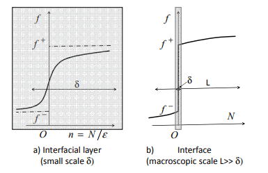
On the contrary, there is the question of the scale of observation. The interface appears as a discontinuity surface on a macroscopic scale, but may become a continuous medium on a smaller scale. Moreover, if we observe it on an even smaller scale, the continuity gives way to atomic and molecular discontinuities and their constituents, the elementary particles (Rocard 1933; Roussel 2016).
For a mechanical physicist, the macroscopic description is required to model a problem. However, the mechanical physicist must sometimes go down to a very small scale within the objects to understand their behavior. This is true for both interfaces and bulks. The mechanical physicist and thermodynamician willingly explore the molecular level to understand the behavior of gases, liquids or solids. The application of the laws of mechanics to objects at a molecular level makes it possible to establish macroscopic constitutive laws of mechanics for continuous media through the statistical theories that use approximations. These scientists commonly use Boltzmann’s equation, Fermi’s theory and the BBGKY hierarchy. The experimental measurements provide the data that allows them to use the modeling techniques developed from these laws.
It is the same for interfaces. These interfaces can be considered as surfaces with physical properties on a macroscopic scale, but if we examine them on a smaller scale, using powerful microscopes, we will see many differences. Whether or not we go as far as the molecular level, there is indeed a thickness to what appears to be a simple geometric surface. Thus, it is useful to talk about interfacial thickness and an interfacial zone – or an interfacial layer – when we study the interior of an interface in detail (Gatignol and Prud’homme 2001). This exploration will be carried out on a single scale, that of thickness, i.e. in the direction normal to the surface. Thus, the scales in the other directions that are tangential to the surface are left unchanged.
As we have already seen in Sect. 4.1.3, Euler’s equation emerges from the Navier-Stokes equation (4.8a, $4.8 \mathrm{~b})$ for $R e=\infty$. However Euler’s equation is also a special case of Cauchy’s equation (2.38) if we use the particular constitutive relation for inviscid fluids (3.9). Euler’s equation then reads $$ \varrho \frac{\mathrm{D} u_{i}}{\mathrm{D} t}=\varrho k_{i}+\frac{\partial}{\partial x_{j}}\left(-p \delta_{i j}\right) $$ or
$$ \varrho \frac{\mathrm{D} u_{i}}{\mathrm{D} t}=\varrho k_{i}-\frac{\partial p}{\partial x_{i}} $$ and it holds without restriction for all inviscid flows. In symbolic notation we write $$ \varrho \frac{\mathrm{D} \vec{u}}{\mathrm{D} t}=\varrho \vec{k}-\nabla p $$ We derive Euler’s equations in natural coordinates from (4.40b) by inserting the acceleration in the form (1.24). Relative to the basis vectors $\vec{t}$ in the direction of the pathline, $\vec{n}{\sigma}$ in the principle normal direction and $\vec{b}{\sigma}$ in the binormal direction, the vectors $\nabla p$ and $\vec{k}$ are $$ \begin{gathered} \nabla p=\frac{\partial p}{\partial \sigma} \vec{t}+\frac{\partial p}{\partial n} \vec{n}{\sigma}+\frac{\partial p}{\partial b} \vec{b}{\sigma} \ \vec{k}=k_{\sigma} \vec{t}+k_{n} \vec{n}{\sigma}+k{b} \vec{b}{\sigma} \end{gathered} $$ and the component form of Euler’s equation in natural coordinates, with $u=|\vec{u}|$, becomes $$ \begin{aligned} \frac{\partial u}{\partial t}+u \frac{\partial u}{\partial \sigma} &=k{\sigma}-\frac{1}{\varrho} \frac{\partial p}{\partial \sigma} \ \frac{u^{2}}{R} &=k_{n}-\frac{1}{\varrho} \frac{\partial p}{\partial n} \ 0 &=k_{b}-\frac{1}{\varrho} \frac{\partial p}{\partial b} \end{aligned} $$
物理代写|流体力学代写Fluid Mechanics代考|Bernoulli’s Equation
Under mildly restricting assumptions it is possible to find so-called first integrals of Euler’s equations, which then represent conservation laws. The most important first integral of Euler’s equations is Bernoulli’s equation. We assume that the mass body force has a potential $(\vec{k}=-\nabla \psi)$, i.e., $\psi=-g_{i} x_{i}$ for the gravitational force. We multiply Euler’s equation (4.40a) by $u_{i}$, thus forming the inner product with $\vec{u}$, and obtain the relation $$ u_{i} \frac{\partial u_{i}}{\partial t}+u_{i} u_{j} \frac{\partial u_{i}}{\partial x_{j}}=-\frac{1}{\varrho} u_{i} \frac{\partial p}{\partial x_{i}}-u_{i} \frac{\partial \psi}{\partial x_{i}} $$ After transforming the second term on the left-hand side and relabelling the dummy indices, this becomes $$ u_{j} \frac{\partial u_{j}}{\partial t}+u_{j} \frac{\partial}{\partial x_{j}}\left[\frac{u_{i} u_{i}}{2}\right]=-\frac{1}{\varrho} u_{j} \frac{\partial p}{\partial x_{j}}-u_{j} \frac{\partial \psi}{\partial x_{j}} $$ We could, in principle, integrate this equation along an arbitrary smooth curve, but we arrive at a particularly simple and important result if we integrate along a streamline. With $u=|\vec{u}|$, from the differential equation for the streamline (1.11), we have
$$ u_{j}=u \mathrm{~d} x_{j} / \mathrm{d} s, $$ so that $$ u_{j} \frac{\partial}{\partial x_{j}}=u \frac{\mathrm{d} x_{j}}{\mathrm{~d} s} \frac{\partial}{\partial x_{j}}=u \frac{\mathrm{d}}{\mathrm{d} s} $$ holds, and because $u_{j} \partial u_{j} / \partial t=u \partial u / \partial t$ we can write for (4.53) $$ \frac{\partial u}{\partial t}+\frac{\mathrm{d}}{\mathrm{d} s}\left[\frac{u^{2}}{2}\right]=-\frac{1}{\varrho} \frac{\mathrm{d} p}{\mathrm{~d} s}-\frac{\mathrm{d} \psi}{\mathrm{d} s} $$ Integration along the arc length of the streamline leads us to Bernoulli’s equation in the form $$ \int \frac{\partial u}{\partial t} \mathrm{~d} s+\frac{u^{2}}{2}+\int \frac{\mathrm{d} p}{\varrho}+\psi=C $$ or integrating from the initial point $A$ to the final point $B$ we get the definite integral $$ \int_{A}^{B} \frac{\partial u}{\partial t} \mathrm{~d} s+\frac{1}{2} u_{B}^{2}+\int_{A}^{B} \frac{1}{\varrho} \frac{\mathrm{d} p}{\mathrm{~d} s} \mathrm{~d} s+\psi_{B}=\frac{1}{2} u_{A}^{2}+\psi_{A} $$
物理代写|流体力学代写Fluid Mechanics代考|Vortex Theorems
We shall now consider the circulation of a closed material line as it was introduced by (1.105) $$ \Gamma=\oint_{(C(t))} \vec{u} \cdot \mathrm{d} \vec{x} . $$ Its rate of change is calculated using (1.101) to give $$ \frac{\mathrm{D} \Gamma}{\mathrm{D} t}=\frac{\mathrm{D}}{\mathrm{D} t} \oint_{(C(t))} \vec{u} \cdot \mathrm{d} \vec{x}=\oint_{(C)} \frac{\mathrm{D} \vec{u}}{\mathrm{D} t} \cdot \mathrm{d} \vec{x}+\oint_{(C)} \vec{u} \cdot \mathrm{d} \vec{u} . $$ The last closed integral vanishes, since $\vec{u} \cdot \mathrm{d} \vec{u}=\mathrm{d}(\vec{u} \cdot \vec{u} / 2)$ is a total differential of a single valued function, and the starting point of integration coincides with the end point.
We now follow on with the discussion in connection with Eq. (1.102), and seek the conditions for the time derivative of the circulation to vanish. It has already been shown that in these circumstances the acceleration $\mathrm{D} \vec{i} / \mathrm{D} t$ must have a potential $I$, but this is not the central point of our current discussion.
Using Euler’s equation $(4.40 \mathrm{a}, 4.40 \mathrm{~b})$ we acquire the rate of change of the line integral over the velocity vector in the form $$ \frac{\mathrm{D} \Gamma}{\mathrm{D} t}=\oint_{(C)} \vec{k} \cdot \mathrm{d} \vec{x}-\oint_{(C)} \frac{\nabla p}{\varrho} \cdot \mathrm{d} \vec{x} $$ and conclude from this that $\mathrm{D} \Gamma / \mathrm{D} t$ vanishes if $\vec{k} \cdot \mathrm{d} \vec{x}$ and $(\nabla p / \varrho) \cdot \mathrm{d} \vec{x}$ can be written as total differentials. If the mass body force $\vec{k}$ has a potential the first closed integral is zero because $$ \vec{k} \cdot \mathrm{d} \vec{x}=-\nabla \dot{\psi} \cdot \mathrm{d} \vec{x}=-\mathrm{d} \psi . $$ In a homogeneous density field or in barotropic flow, because of $$ \frac{\nabla p}{\varrho} \cdot \mathrm{d} \vec{x}=\frac{\mathrm{d} p}{\varrho(p)}=\mathrm{d} P $$
the second integral also vanishes. The last three equations form the content of Thomson’s vortex theorem or Kelvin’s circulation theorem $$ \frac{\mathrm{D} \Gamma}{\mathrm{D} t}=0 . $$
We start with a Newtonian fluid which is defined by the constitutive relation (3.1) and, by setting (3.1) and (1.29) into (2.38), we obtain the Navier-Stokes equations $$ \varrho \frac{\mathrm{D} u_{i}}{\mathrm{D} t}=\varrho k_{i}+\frac{\partial}{\partial x_{i}}\left{-p+\lambda^{*} \frac{\partial u_{k}}{\partial x_{k}}\right}+\frac{\partial}{\partial x_{j}}\left{\eta\left[\frac{\partial u_{i}}{\partial x_{j}}+\frac{\partial u_{j}}{\partial x_{i}}\right]\right} $$ where we have used the exchange property of the Kronecker delta $\delta_{i j}$. With the linear law for the friction stresses (3.2) and the linear law for the heat flux vector (3.8), we specialize the energy equation to the case of Newtonian fluids $$ \varrho \frac{\mathrm{D} e}{\mathrm{D} t}-\frac{p}{\varrho} \frac{\mathrm{D} \varrho}{\mathrm{D} t}=\Phi+\frac{\partial}{\partial x_{i}}\left[\lambda \frac{\partial T}{\partial x_{i}}\right] $$ where the dissipation function $\Phi$ is given hy (3.6). In the same way we deal with the forms (2.116) and (2.118) of the energy equation, which are often more appropriate. Another useful form of the energy equation arises by inserting the enthalpy $h=e+p / \varrho$ into (4.2). Because of
$$ \varrho \frac{\mathrm{D} h}{\mathrm{D} t}=\varrho \frac{\mathrm{D} e}{\mathrm{D} t}-\frac{p}{\varrho} \frac{\mathrm{D} \varrho}{\mathrm{D} t}+\frac{\mathrm{D} p}{\mathrm{D} t} $$ (4.2) can also be written as $$ \varrho \frac{\mathrm{D} h}{\mathrm{D} t}-\frac{\mathrm{D} p}{\mathrm{D} t}=\Phi+\frac{\partial}{\partial x_{i}}\left[\lambda \frac{\partial T}{\partial x_{i}}\right] $$ As a consequence of Gibbs’ relation (2.133), the entropy equation for Newtonian fluids can also appear in place of (4.2) $$ \varrho T \frac{\mathrm{D} s}{\mathrm{D} t}=\Phi+\frac{\partial}{\partial x_{i}}\left[\lambda \frac{\partial T}{\partial x_{i}}\right] $$ If we choose the energy equation (4.2), together with the continuity equation and the Navier-Stokes equations we have five partial differential equations with seven unknown functions. But both the thermal equation of state $p=p(\varrho, T)$ and the caloric equation of state $e=e(\varrho, T)$ appear also. This set of equations forms the starting point for the calculation of frictional compressible flow.
物理代写|流体力学代写Fluid Mechanics代考|Vorticity Equation
Since a viscous incompressible fluid behaves like an inviscid fluid in regions where $\vec{\omega}=0$, the question arises of what the differential equation for the distribution of $\vec{\omega}$ is. Of course this question does not arise if we consider the velocity field as given, because then $\vec{\omega}$ can be calculated directly from the velocity field using Eq. (1.49). To obtain the desired relation, we take the curl of the Eg. (4.9b). For reasons of clarity, we shall use symbolic notation here. We assume further that $\vec{k}$ has a potential $(\vec{k}=-\nabla \psi)$, and use the identity (4.11) in Eq. (4.9b). In addition, we make use of (1.78) to obtain the Navier-Stokes equations in the form $$ \frac{1}{2} \frac{\partial \vec{u}}{\partial t}-\vec{u} \times \vec{\omega}=-\frac{1}{2} \nabla\left[\psi+\frac{p}{\varrho}+\frac{\vec{u} \cdot \vec{u}}{2}\right]-\nu \nabla \times \vec{\omega} $$ The operation $\nabla \times$ applied to (4.12), along with the identity (easily verified in index notation) $$ \nabla \times(\vec{u} \times \vec{\omega})=\vec{\omega} \cdot \nabla \vec{u}-\vec{u} \cdot \nabla \vec{\omega}-\vec{\omega} \nabla \cdot \vec{u}+\vec{u} \nabla \cdot \vec{\omega} $$ furnishes the new left-hand side $\partial \vec{\omega} / \partial t-\vec{\omega} \cdot \nabla \vec{u}+\vec{u} \cdot \nabla \vec{\omega}$, where we have already noted that the flow is incompressible $(\nabla \cdot \vec{u}=0)$ and that the divergence of the curl always vanishes $$ 2 \nabla \cdot \vec{\omega}=\nabla \cdot(\nabla \times \vec{u})=0 $$ This can be shown in index notation or simply explained by the fact that the symbolic vector $\nabla$ is orthogonal to $\nabla \times \vec{u}$. On the right-hand side of (4.12), the term in parantheses vanishes, since the symbolic vector $\nabla$ is parallel to the gradient. The remaining term on the right-hand side $-\nu \nabla \times(\nabla \times \vec{\omega})$ is recast using the identity (4.10), and because $\nabla \cdot \vec{\omega}=0$ from (4.14) we extract the new right-hand side $\nu \Delta \vec{\omega}$. In this manner we arrive at the vorticity equation
$$ \frac{\partial \vec{\omega}}{\partial t}+\vec{u} \cdot \nabla \vec{\omega}=\vec{\omega} \cdot \nabla \vec{u}+\nu \Delta \vec{\omega} $$ Because $\partial / \partial t+\vec{u} \cdot \nabla=\mathrm{D} / \mathrm{D} t$ we can shorten this to $$ \frac{\mathrm{D} \vec{\omega}}{\mathrm{D} t}=\vec{\omega} \cdot \nabla \vec{u}+\nu \Delta \vec{\omega} . $$
物理代写|流体力学代写Fluid Mechanics代考|Effect of Reynolds’ Number
In viscous flow, the term, $\nu \Delta \vec{\omega}$ in (4.16) represents the change in the angular velocity of a material particle which is due to its neighboring particles. Clearly, the particle is set into rotation by its neighbors via viscous torques, and it itself exerts torques on other neighboring particles, thus setting these into rotation. The particle only passes on the vector of angular velocity $\vec{\omega}$ on to the next one, just as temperature is passed on by heat conduction, or concentration by diffusion. Thus we speak of the “diffusion” of the angular velocity vector $\vec{\omega}$ or of the vorticity vector curl $\vec{u}=\nabla \times \vec{u}=2 \vec{\omega}$. From what we have said before, we conclude that angular velocity cannot be produced within the interior of an incompressible fluid, but gets there by diffusion from the boundaries of the fluid region. Flow regions where the diffusion of the vorticity vector is negligible can be treated according to the rules of inviscid and irrotational fluids.
As we know, equations which express physical relationships and which are dimensionally homogeneous (only these are of interest in engineering) must be reducible to relations hetween dimensionless quantities. Ising the typical velocity $U$ of the problem, the typical length $L$ and the density $\varrho$, constant in incompressible flow, we introduce the dimensionless dependent variables
$$ \begin{aligned} u_{i}^{+} &=\frac{u_{i}}{U} \ p^{+} &=\frac{p}{\varrho U^{2}} \end{aligned} $$ and the independent variables $$ \begin{aligned} x_{i}^{+} &=\frac{x_{i}}{L} \ t^{+} &=t \frac{U}{L} \end{aligned} $$ into the Navier-Stokes equations, and obtain (neglecting body forces) $$ \frac{\partial u_{i}^{+}}{\partial t^{+}}+u_{j}^{+} \frac{\partial u_{i}^{+}}{\partial x_{j}^{+}}=-\frac{\partial p^{+}}{\partial x_{i}^{+}}+R e^{-1} \frac{\partial^{2} u_{i}^{+}}{\partial x_{j}^{+} \partial x_{j}^{+}} $$ where $R e$ is the already known Reynolds’ number $$ R e=\frac{U L}{\nu} $$
物理代写|流体力学代写Fluid Mechanics代考|Equations of Motion for Particular
物理代写|流体力学代写Fluid Mechanics代考|Constitutive Relations for Fluids
物理代写|流体力学代写Fluid Mechanics代考|already explained in the previous
As already explained in the previous chapter on the fundamental laws of continuum mechanics, bodies behave in such a way that the universal balances of mass, momentum, energy and entropy are satisfied. Yet only in very few cases, like, for example, the idealizations of a point mass or of a rigid body without heat conduction, are these laws enough to describe a body’s behavior. In these special cases, the characteristics of “mass” and “mass distribution” belonging to each body are the only important features. In order to describe a deformable medium, the material from which it is made must be characterized, because clearly, the deformation or the rate of deformation under a given load is dependent on the material. Because the balance laws yield more unknowns than independent equations, we can already conclude that a specification of the material through relationships describing the way in which the stress and heat flux vectors depend on the other field quantities is generally required. Thus the balance laws yield more unknowns than independent equations. The summarizing list of the balance laws of mass (2.2) $$ \frac{\partial \varrho}{\partial t}+\frac{\partial}{\partial x_{i}}\left(\varrho u_{i}\right)=0 $$ of momentum (2.38) $$ \varrho \frac{D u_{i}}{D t}=\varrho k_{i}+\frac{\partial \tau_{j i}}{\partial x_{j}} $$ of angular momentum (2.53) $$ \tau_{i j}=\tau_{j i} $$
and of energy (2.119) $$ \varrho \frac{D e}{D t}=\tau_{i j} \frac{\partial u_{i}}{\partial x_{j}}-\frac{\partial q_{i}}{\partial x_{i}} $$ yield 17 unknown functions $\left(\varrho, u_{i}, \tau_{i j}, q_{i}, e\right)$ in only eight independently available equations. Instead of the energy balance, we could also use the entropy balance (2.134) here, which would introduce the unknown function $s$ instead of $e$, but by doing this the number of equations and unknown functions would not change. Of course we could solve this system of equations by specifying nine of the unknown functions arbitrarily, but the solution found is then not a solution to a particular technical problem.
物理代写|流体力学代写Fluid Mechanics代考|The final condition
The final condition is here of particular importance, since, as we know from Sect. $2.4$, the equations of motion (momentum balance) are not frame independent in this sense. In accelerating reference frames, the apparent forces are introduced, and only the axiom of objectivity ensures that this remains the only difference for the transition from an inertial system to a relative system. However, it is clear that an observer in an accelerating reference frame detects the same material properties as an observer in an inertial system. To illustrate this, for a given deflection of a massless spring, an observer in a rotating reference frame would detect exactly the same force as in an inertial frame.
In so-called simple fluids, the stress on a material point at time $t$ is determined by the history of the deformation involving only gradients of the first order or more exactly, by the relative deformation tensor (relative Cauchy-Green-tensor) as every fluid is isotropic. Essentially all non-Newtonian fluids belong to this group.
The most simple constitutive relation for the stress tensor of a viscous fluid is a linear relationship between the components of the stress tensor $\tau_{i j}$ and those of the rate of deformation tensor $e_{i j}$. Almost trivially, this constitutive relation satisfies all the above axioms. The material theory shows that the most gêneraal linéar rèlationship of this kind must be of the form $$ \tau_{i j}=-p \delta_{i j}+\lambda^{} e_{k k} \delta_{i j}+2 \eta e_{i j} $$ or, using the unit tensor $\mathbf{I}$ $$ \mathbf{T}=\left(-p+\hat{\lambda}^{} \nabla \cdot \vec{u}\right) \mathbf{I}+2 \eta \mathbf{E} $$ (Cauchy-Poisson law), so that noting the decomposition (2.35), the tensor of the friction stresses is given by $$ P_{i j}=\lambda^{*} e_{k k} \delta_{i j}+2 \eta e_{i j} $$
or $$ \mathbf{P}=\lambda^{} \nabla \cdot \vec{u} \mathbf{I}+2 \eta \mathbf{E} $$ We next note that the friction stresses at the position $\vec{x}$ are given by the rate of deformation tensor $e_{i j}$ at $\vec{x}$, and are not explicitly dependent on $\vec{x}$ itself. Since the friction stress tensor $P_{i j}$ at $\vec{x}$ determines the stress acting on the material particle at $\vec{x}$, we conclude that the stress on the particle only depends on the instantaneous value of the rate of deformation tensor and is not influenced by the history of the deformation. We remind ourselves that for a fluid at rest or for a fluid undergoing rigid body motion, $e_{i j}=0$, and (3.1a) reduces to (2.33). The quantities $\lambda^{}$ and $\eta$ are scalar functions of the thermodynamic state, typical to the material. Thus (3.1a, $3.1 \mathrm{~b})$ is the generalization of $\tau=\eta \dot{\gamma}$, which we have already met in connection with simple shearing flow and defines the Newtonian fluid.
The extraordinary importance of the linear relationship ( $3.1 \mathrm{a}, 3.1 \mathrm{~b})$ lies in the fact that it describes the actual material behavior of most technically important fluids very well. This includes practically all gases, in particular air and steam, gas mixtures and all liquids of low molecular weight, like water, and also all mineral oils.
物理代写|流体力学代写Fluid Mechanics代考|Here k is a positive function of the thermodynamic
Here $\lambda$ is a positive function of the thermodynamic state, and is called the thermal conductivity. The minus sign here is in agreement with the inequality (2.141). Experiments show that this linear law describes the actual behavior of materials very well. The dependency of the thermal conductivity on $p$ and $T$ remains open in (3.8), and has to be determined experimentally. For gases the kinetic theory leads to the result $\lambda \sim \eta$, so that the thermal conductivity shows the same temperature dependence as the shear viscosiry. (For liquids, one discovers theorerically thar the thermal conductivity is proportional to the velocity of sound in the fluid.)
In the limiting case $\eta, \lambda^{}=0$, we extract from the Cauchy-Poisson law the constitutive relation for inviscid fluids $$ \tau_{i j}=-p \delta_{i j} $$ Thus, as with a fluid at rest, the stress tensor is only determined by the pressure $p$. As far as the stress state is concerned, the limiting case $\eta, \lambda^{}=0$ leads to the sảmé result as $e_{i j}=0$. Also consistênt with $\eta, \lambda^{*}=0$ is the casse $\lambda=0$; ignoring the friction stresses implies that we should in general also ignore the heat conduction. It would now appear that there is no technical importance attached to the condition $\eta, \lambda *, \lambda=0$. Yet the opposite is actually the case. Many technically important, real flows are described very well using this assumption. This has already been stressed in connection with the flow through turbomachines. Indeed the flow past a flying object can often be predicted using the assumption of inviscid flow. The reason for this can be clearly seen when we note that fluids which occur in applications (mostly air or water) only have “small” viscosities. However, the viscosity is a dimensional quantity, and the expression “small viscosity” is vague, since the numerical value of the physical quantity “viscosity” may be arbitrarily changed by suitable choice of the units in the dimensional formula. The question of whether the viscosity is small or not can only be settled in connection with the specific problem, however this is already possible using simple dimensional arguments. For incompressible fluids, or by using Stokes’ relation (3.5), only the shear viscosity appears in the constitutive relation (3.1a, 3.1b). If, in addition, the temperature field is homogeneous, no thermodynamic quantities enter the problem, and the incident flow is determined by the velocity $U$, the density $\varrho$ and the shear viscosity $\eta$. We characterize the body past which the fluid flows by its typical length $L$, and we form the dimensionless quantity $$ R e=\frac{U L \varrho}{\eta}=\frac{U L}{v} $$
物理代写|流体力学代写Fluid Mechanics代考|Constitutive Relations for Fluids
τ一世j=−pd一世j因此,与静止的流体一样,应力张量仅由压力决定p. 就应力状态而言,极限情况这,λ=0导致 sảmé 结果为和一世j=0. 也符合这,λ∗=0是案例λ=0; 忽略摩擦应力意味着我们通常也应该忽略热传导。 现在看来,该条件没有技术重要性这,λ∗,λ=0. 然而事实恰恰相反。许多技术上重要的、真实的流量都使用这个假设很好地描述了。这已经在与流过涡轮机有关的情况下得到强调。实际上,通常可以使用无粘性流动的假设来预测经过飞行物体的流动。当我们注意到应用中出现的流体(主要是空气或水)只有“小”粘度时,就可以清楚地看到其原因。However, the viscosity is a dimensional quantity, and the expression “small viscosity” is vague, since the numerical value of the physical quantity “viscosity” may be arbitrarily changed by suitable choice of the units in the dimensional formula. 粘度是否小,只能结合具体问题来解决,然而,这已经可以使用简单的维度参数来实现。对于不可压缩流体,或通过使用斯托克斯关系(3.5),只有剪切粘度出现在本构关系(3.1a,3.1b)中。此外,如果温度场是均匀的,则没有热力学量进入问题,入射流由速度决定在, 密度ϱ和剪切粘度这. 我们通过其典型长度来描述流体流过的物体大号,我们形成无量纲量
物理代写|流体力学代写Fluid Mechanics代考|Momentum and Angular Momentum
物理代写|流体力学代写Fluid Mechanics代考|Accelerating Frame
The balance of momentum and angular momentum that we have discussed so far are only valid in inertial reference frames. An inertial reference frame in classical mechanics could be a Cartesian coordinate system whose axes are fixed in space (relative, for example, to the fixed stars), and which uses the average solar day as a unit of time, the basis of all our chronology. All reference frames which move uniformly, i.e.., not acceelerrating in this systêm, arre equivallênt añd thus aree inertiāl frames.
The above balances do not hold in frames which are accelerating relative to an inertial frame. But the forces of inertia which arise from nonuniform motion of the frame are often so small that reference frames can by regarded as being approximately inertial frames. On the other hand, we often have to use reference frames where such forces of inertia cannot be neglected.
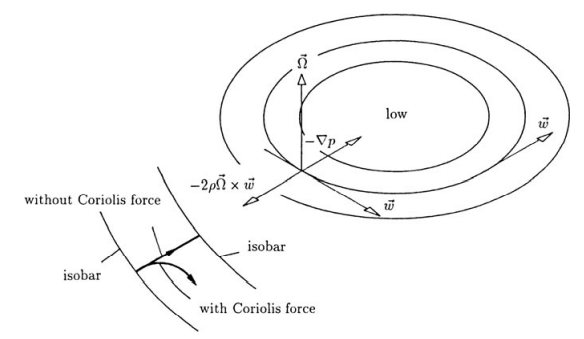
To illustrate this we will look at a horizontal table which is rotating with angular velocity $\Omega$. On the table and rotating with it is an observer, who is holding a string at the end of which is a stone, lying a distance $R$ from the fulcrum of the table. The observer experiences a force (the centrifugal force) in the string. Since the stone is at rest in his frame, and therefore the acceleration in his reference frame is zero, the rate of change of momentum must also be zero, and thus, by the balance of momentum (2.9), the force in the string should vanish. The observer then correctly concludes that the balance of momentum does not hoold in his reference frame. The rotating table must be treated as an noninertial reference frame. The source of the force in the string is obvious to an observer who is standing beside the rotating table. He sees that the stone is moving on a circular path and so it experiences an acceleration toward the center of the circle, and that according to the balance of momentum, there must be an external force acting on the stone. The acceleration is the centripetal acceleration, which is given here by $\Omega^{2} \mathrm{R}$. The force acting inwards is the centripetal force which is exactly the same size as the centrifugal force experienced by the rotating observer.
In this example the reference frame of the observer at rest, that is the earth, can be taken as an inertial reference frame. Yet in other cases deviations from what is expected from the balance of momentum appear. This is because the earth is rotating and therefore the balance of momentum strictly does not hold in a reference frame moving with the earth. With respect to a frame fixed relative to the earth we observe, for example, the deflection of a free falling body to the east, or the way that the plane of oscillation of Foucault’s pendulum rotates. These examples, and many others, are not compatible with the validity of the balance of momentum in the reference frame chosen to be the earth. For most terrestrial events, however, a coordinate system whose origin is at the center of the earth, and whose axes are directed towards the fixed stars, is valid as an inertial reference frame. The easterly deflection mentioned above can then be explained by the fact that the body, in its initial position, has a somewhat higher circumferential speed because of the rotation of the earth than at the impact point nearer the center of the earth. To explain Foucault’s pendulum, we notice that, in agreement with (2.9), the pendulum maintains its plane of oscillation relative to the inertial frame. The reference frame attached to the earth rotates about this plane, and an observer in the laboratory experiences a rotation of the plane of oscillation relative to his system with a period of twenty-four hours.
物理代写|流体力学代写Fluid Mechanics代考|Applications to Turbomachines
Typical applications of the balances of momentum and of angular momentum can be found in the theory of turbomachines. The essential element present in all turbomachines is a rotor equipped with blades surrounding it, either in the axial or radial direction.
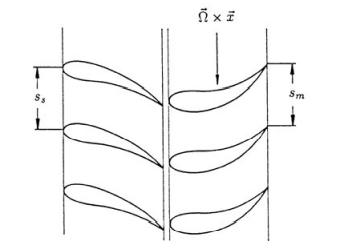
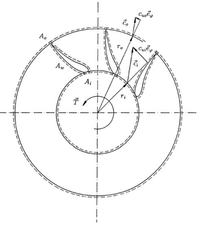
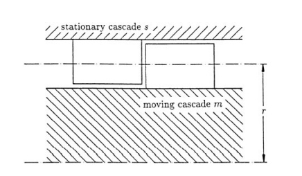
When the fluid exerts a force on the moving blades, the fluid does work. In this case we can also speak of turbo force machines (turbines, wind wheels, etc.). If the moving blades exert a force on the fluid, and thus do work on it, increasing its energy, we speak of turbo work machines (fans, compressors, pumps, propellers). Often the rotor has an outer casing, called stator, which itself is lined with blades. Since these blades are fixed, no work is done on them. Their task is to direct the flow either towards or away from the moving blades attached to the rotor. These blades are called guide blades or guide vanes. A row of fixed blades together with a row of moving blades is called a stage. A turbomachine can be constructed with one or more of these stages. If the cylindrical surface of Fig. $2.6$ at radius $r$ through the stage is cut and straightened, the contours of the blade sections originally on the cylindrical surface form two straight cascades. The set up shown consists of a
turbine stage where the fixed cascade is placed before the moving cascade seen in the direction of the flow.
Obviously the cascades are used to turn the flow. If the turning is such that the magnitude of the velocity is not changed, the cascade is a pure turning or constant pressure cascade, since then no change of pressure occurs through the cascade (only in the case of frictionless flow). In general the magnitude of the velocity changes with the turning and therefore also the pressure. If the magnitude of the velocity is increased we have an acceleration cascade, typically found in turbines, and if it is decreased we have a deceleration cascade, typically found in compressors. We shall consider the cascade to be a strictly periodic ordering of blades, that is, an infinitely long row of blades with exactly the same spacing $s$ between blades along the cascade. Because of this the flow is also strictly periodic.
物理代写|流体力学代写Fluid Mechanics代考|Balance of Energy
The fact that mechanical energy can be changed into heat and heat can be changed into mechanical energy shows that the balance laws of mechanics we have discussed up to now are not enough for a complete description of the motion of a fluid. As well as the two laws we have already treated, therefore a third basic empirical law, the balance of energy, appears: The rate of change of the total energy of a body is equal to the power of the external forces plus the rate at which heat is transferred to the body. This law can be “deduced” from the well known first law of thermodynamics together with a mechanical energy equation which follows from Cauchy’s Eq. (2.38a, 2.38b). However here we prefer to postulate the balance of the total energy, and to infer from it the more restrictive statement of the first law of thermodynamics.
We shall assume the fundamentals of classical thermodynamics as known. Thermodynamics is concerned with processes where the material is at rest and where all quantities appearing are independent of position (homogeneous), and therefore are only dependent on time. An important step to the thermodynamics of irreversible processes as they appear in the motion of fluids, consists of simply applying the classical laws to a material particle. If $e$ is the internal energy per unit
mass, then the internal energy of a material particle is given by $e \mathrm{~d} m$, and we can calculate the internal energy $E$ of a body, that is, the energy of a bounded part of the fluid, as the integral over the region occupied by the body $$ E=\iiint_{(V(t))} e \varrho \mathrm{d} V $$ In order to obtain the total energy of the fluid body under consideration, the kinetic energy which does not appear in the classical theory must be added to (2.109). The kinetic energy of the material particle is $\left(u^{2} / 2\right) \mathrm{d} m$, and the kinetic energy $K$ of the body is correspondingly $$ K=\iiint_{(V(t))} \frac{u_{i} u_{i}}{2} \varrho \mathrm{d} V $$ The applied forces which appear are the surface and body forces which were discussed in the context of the balance of momentum. The power of the surface force $\vec{t} \mathrm{~d} S$ is $\vec{u} \cdot \vec{t} \mathrm{~d} S$, while that of the body force $\varrho \vec{k} \mathrm{~d} V$ is $\vec{u} \cdot \vec{k} \varrho \mathrm{d} V$. The power of the applied forces is then $$ P=\iiint_{(V(t))} \varrho u_{i} k_{i} \mathrm{~d} V+\iint_{(S(t))} u_{i} t_{i} \mathrm{~d} S $$ In analogy to the volume flow $\vec{u} \cdot \vec{n} \mathrm{~d} S$ through an element of the surfacee, we introduce the heat flux through an element of the surface with $-\vec{q} \cdot \vec{n} \mathrm{~d} S$ and denote $\vec{q}$ as the heat flux vector. The minus sign is chosen so that inflowing energy ( $\vec{q}$ and $\vec{n}$ forming an obtuse angle) is counted as positive. From now we shall limit ourselves to the transfer of heat by conduction, although $\vec{q}$ can also contain other kinds of heat transfer, for example, heat transfer by radiation, via Poynting’s vector.
物理代写|流体力学代写Fluid Mechanics代考|Momentum and Angular Momentum
物理代写|流体力学代写Fluid Mechanics代考|Fundamental Laws of Continuum
物理代写|流体力学代写Fluid Mechanics代考|Conservation of Mass, Equation of Continuity
Conservation of mass has already been postulated in the last chapter, and now we will make use of our earlier results and employ (1.83) and (1.93) to change the conservation law (1.85) to the form $$ \frac{\mathrm{D}}{\mathrm{D} t} \iiint_{(V(t))} \varrho \mathrm{d} V=\iiint_{(V)}\left[\frac{\partial \varrho}{\partial t}+\frac{\partial}{\partial x_{i}}\left(\varrho u_{i}\right)\right] \mathrm{d} V=0 $$ This equation holds for every volume that could be occupied by the fluid, that is, for arbitrary choice of the integration region $(V)$. We could therefore shrink the integration region to a point, and we conclude that the continuous integrand must itself vanish at every $\vec{x}$. Thus we are led to the local or differential form of the law of conservation of mass $$ \frac{\partial \varrho}{\partial t}+\frac{\partial}{\partial x_{i}}\left(\varrho u_{i}\right)=0 $$ This is the continuity equation. If we use the material derivative (1.20) we obtain $$ \frac{\mathrm{D} \varrho}{\mathrm{D} t}+\varrho \frac{\partial u_{i}}{\partial x_{i}}=0 $$ or written symbolically $$ \frac{\mathrm{D} \varrho}{\mathrm{D} t}+\varrho \nabla \cdot \vec{u}=0 $$
物理代写|流体力学代写Fluid Mechanics代考|Balance of Momentum
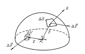
As the first law (axiom) of classical mechanics, accepted to be true without proof but embracing our experience, we state the momentum balance: in an inertial frame the rate of change of the momentum of a body is balanced by the force applied on this body $$ \frac{\mathrm{D} \vec{P}}{\mathrm{D} t}=\vec{F} $$ What follows now only amounts to rearranging this axiom explicitly. The body is still a part of the fluid which always consists of the same material points. Analogous to ( $1.83)$, we calculate the momentum of the body as the integral over the region occupied by the body $$ \vec{P}=\iiint_{(V(t))} \varrho \vec{u} \mathrm{~d} V $$ The forces affecting the body basically fall into two classes, body forces, and surface or contact forces. Body forces are forces with a long range of influence which act on all the material particles in the body and which, as a rule, have their source in fields of force. The most important example we come across is the earth’s gravity field. The gravitational field strength $\vec{g}$ acts on every molecule in the fluid particle, and the sum of all the forces acting on the particle represents the actual gravitational force
$$ \Delta \vec{F}=\vec{g} \sum_{i} m_{i}=\vec{g} \Delta m $$ The force of gravity is therefore proportional to the mass of the fluid particle. As before, in the framework of the continuum hypothesis, we consider the body force as a continuous function of mass or volume and call $$ \vec{k}=\lim {\Delta m \rightarrow 0} \frac{\Delta \vec{F}}{\Delta m} $$ the mass body force; in the special case of the earth’s gravitational field $\vec{k}=\vec{g}$, we call it the gravitational force. The volume body force is the force referred to the volume, thus $$ \vec{f}=\lim {\Delta V \rightarrow 0} \frac{\Delta \vec{F}}{\Delta V} $$ (cf. Fig. 2.1), and in the special case of the gravitational force we get $$ \vec{f}=\lim _{\Delta V \rightarrow 0} \vec{g} \frac{\Delta m}{\Delta V}=\vec{g} \varrho . $$
物理代写|流体力学代写Fluid Mechanics代考|Balance of Angular Momentum
As the second general axiom of classical mechanics we shall discuss the angular momentum balance. This is independent of the balance of linear momentum. In an inertial frame, the rate of change of the angular momentum is equal to the moment of the external forces acting on the body $$ \frac{\mathrm{D}}{\mathrm{D} t}(\vec{L})=\vec{M} . $$ We calculate the angular momentum $\vec{L}$ as the integral over the region occupied by the fluid body $$ \vec{L}=\iiint_{(V(t))} \vec{x} \times(\varrho \vec{u}) \mathrm{d} V $$ The angular momentum in $(2.45)$ is taken about the origin such that the position vector is $\vec{x}$, and so we must use the same reference point to calculate the moment of the applied forces $$ \vec{M}=\iiint_{(V(t))} \vec{x} \times(\varrho \vec{k}) \mathrm{d} V+\iint_{(S(t))} \vec{x} \times \vec{t} \mathrm{~d} S $$
recalling, however, that the choice of reference point is up to us. Therefore the law of angular momentum takes the form $$ \frac{\mathrm{D}}{\mathrm{D} t} \iiint_{(V(t))} \vec{x} \times(\varrho \vec{u}) \mathrm{d} V=\iiint_{(V(t))} \vec{x} \times(\varrho \vec{k}) \mathrm{d} V+\iint_{(S)} \vec{x} \times \vec{t} \mathrm{~d} S $$ where, for the same reasons as before, we have replaced the time varying domain of integration on the right with a fixed domain. Now we wish to show that the differential form of the balance of angular momentum implies the symmetry of the stress tensor. We introduce the expression (2.29a, 2.29b) into the surface integral, which can then be written as a volume integral. In index notation this becomes $$ \iint_{(S)} \epsilon_{i j k} x_{j} \tau_{l k} n_{l} \mathrm{~d} S=\iiint_{(V)} \epsilon_{i j k} \frac{\partial}{\partial x_{l}}\left(x_{j} \tau_{l k}\right) \mathrm{d} V $$ and after applying (1.88) to the left-hand side of (2.47) we get first $$ \iiint_{(V)} \epsilon_{i j k}\left(\varrho \frac{\mathrm{D}}{\mathrm{D} t}\left(x_{j} u_{k}\right)-\frac{\partial}{\partial x_{l}}\left(x_{j} \tau_{l k}\right)-x_{j} \varrho k_{k}\right) \mathrm{d} V=0 $$ and after differentiation and combining terms $$ \iiint_{(V)}\left[\epsilon_{i j k} x_{j}\left(\varrho \frac{\mathrm{D} u_{k}}{\mathrm{D} t}-\frac{\partial \tau_{l k}}{\partial x_{l}}-\varrho k_{k}\right)+\varrho \epsilon_{i j k} u_{j} u_{k}-\epsilon_{i j k} \tau_{j k}\right] \mathrm{d} V=0 $$
物理代写|流体力学代写Fluid Mechanics代考|Fundamental Laws of Continuum
物理代写|流体力学代写Fluid Mechanics代考|Material and Spatial Descriptions
Kinematics is the study of the motion of a fluid, without considering the forces which cause this motion, that is without considering the equations of motion. It is natural to try to carry over the kinematics of a mass-point directly to the kinematics of a fluid particle. Its motion is given by the time dependent position vector $\vec{x}(t)$ relative to a chosen origin.
In general we are interested in the motion of a finitely large part of the fluid (or the whole fluid) and this is made up of infinitely many fluid particles. Thus the single particles must remain identifiable. The shape of the particle is no use as an identification, since, because of its ability to deform without limit, it continually changes during the course of the motion. Naturally the linear measure must remain small in spite of the deformation during the motion, something that we guarantee by idealizing the fluid particle as a material point.
For identification, we associate with each material point a characteristic vector $\vec{\xi}$. The position vector $\vec{x}$ at a certain time $t_{0}$ could be chosen, giving $\vec{x}\left(t_{0}\right)=\vec{\xi}$. The motion of the whole fluid can then be described by $$ \vec{x}=\vec{x}(\vec{\xi}, t) \quad \text { or } \quad x_{i}=x_{i}\left(\xi_{j}, t\right) $$
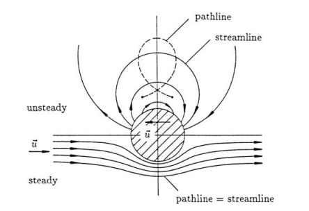
The differential Eq. (1.10) shows that the path of a point in the material is always tangential to its velocity. In this interpretation the pathline is the tangent curve to the velocities of the same material point at different times. Time is the curve parameter, and the material coordinate $\vec{\xi}$ is the family parameter.
Just as the pathline is natural to the material description, so the streamline is natural to the Eulerian description. The velocity field assigns a velocity vector to every place $\vec{x}$ at time $t$ and the streamlines are the curves whose tangent directions are the same as the directions of the velocity vectors. The streamlines provide a vivid description of the flow at time t.
If we interpret the streamlines as the tangent curves to the velocity vectors of different particles in the material at the same instant in time we see that there is no connection between pathlines and streamlines, apart from the fact that they may sometimes lie on the same curve.
By the definition of streamlines, the unit vector $\vec{u} /|\vec{u}|$ is equal to the unit tangent vector of the streamline $\vec{\tau}=\mathrm{d} \vec{x} /|\mathrm{d} \vec{x}|=\mathrm{d} \vec{x} / \mathrm{d} s$ where $\mathrm{d} \vec{x}$ is a vector element of the streamline in the direction of the velocity. The differential equation of the streamline then reads $$ \frac{\mathrm{d} \vec{x}}{\mathrm{~d} s}=\frac{\vec{u}(\vec{x}, t)}{|\vec{u}|}, \quad(t=\text { const }) $$ or in index notation $$ \frac{\mathrm{d} x_{i}}{\mathrm{~d} s}=\frac{u_{i}\left(x_{j}, t\right)}{\sqrt{u_{k} u_{k}}}, \quad(t=\mathrm{const}) $$ Integration of these equations with the “initial condition” that the streamline emanates from a point in space $\vec{x}{0}\left(\vec{x}(s=0)=\vec{x}{0}\right)$ leads to the parametric representation of the streamline $\vec{x}=\vec{x}\left(s, \vec{x}{0}\right)$. The curve parameter here is the arc length $s$ measured from $x{0}$, and the family parameter is $\dot{x}_{0}$.
物理代写|流体力学代写Fluid Mechanics代考|Differentiation with Respect to Time
In the Eulerian description our attention is directed towards events at the place $\vec{x}$ at time $t$. However the rate of change of the velocity $\vec{u}$ at $\vec{x}$ is not generally the acceleration which the point in the material passing through $\vec{x}$ at time $t$ experiences. This is obvious in the case of steady flows where the rate of change at a given place is zero. Yet a material point experiences a change in velocity (an acceleration) when it moves from $\vec{x}$ to $\vec{x}+\mathrm{d} \vec{x}$. Here $\mathrm{d} \vec{x}$ is the vector element of the pathline. The changes felt by a point of the material or by some larger part of the fluid and not the time changes at a given place or region of space are of fundamental importance in the dynamics. If the velocity (or some other quantity) is given in material coordinates, then the material or substantial derivative is provided by (1.6). But if the velocity is given in field coordinates, the place $\vec{x}$ in $\vec{u}(\vec{x}, t)$ is replaced by the path coordinates of the particle that occupies $\vec{x}$ at time $t$, and the derivative with respect to time at fixed $\vec{\xi}$ can be formed from $$ \frac{\mathrm{d} \vec{u}}{\mathrm{~d} t}=\left{\frac{\partial \vec{u}{\vec{x}(\vec{\xi}, t), t}}{\partial t}\right}_{\vec{\xi}} $$
or $$ \frac{\mathrm{d} u_{i}}{\mathrm{~d} t}=\left{\frac{\partial u_{i}\left{x_{j}\left(\xi_{k}, t\right), t\right}}{\partial t}\right}_{\xi_{k}} $$ The material derivative in field coordinates can also be found without direct reference to the material coordinates. Take the temperature field $T(\vec{x}, t)$ as an example: we take the total differential to be the expression $$ \mathrm{d} T=\frac{\partial T}{\partial t} \mathrm{~d} t+\frac{\partial T}{\partial x_{1}} \mathrm{~d} x_{1}+\frac{\partial T}{\partial x_{2}} \mathrm{~d} x_{2}+\frac{\partial T}{\partial x_{3}} \mathrm{~d} x_{3} $$ The first term on the right-hand side is the rate of change of the temperature at a fixed place: the local change. The other three terms give the change in temperature by advancing from $\vec{x}$ to $\vec{x}+\mathrm{d} \vec{x}$. This is the convective change. The last three terms can be combined to give $\mathrm{d} \vec{x} \cdot \nabla T$ or equivalently $\mathrm{d} x_{i} \partial T / \partial x_{i}$. If $\mathrm{d} \vec{x}$ is the vector element of the fluid particle’s path at $\vec{x}$, then (1.10) holds and the rate of change of the temperature of the particle passing $\vec{x}$ (the material change of the temperature) is $$ \frac{\mathrm{d} T}{\mathrm{~d} t}=\frac{\partial T}{\partial t}+\vec{u} \cdot \nabla T $$ or $$ \frac{\mathrm{d} T}{\mathrm{~d} t}=\frac{\partial T}{\partial t}+u_{i} \frac{\partial T}{\partial x_{i}}=\frac{\partial T}{\partial t}+u_{1} \frac{\partial T}{\partial x_{1}}+u_{2} \frac{\partial T}{\partial x_{2}}+u_{3} \frac{\partial T}{\partial x_{3}} $$
物理代写|流体力学代写Fluid Mechanics代考|The Concept of the Continuum and Kinematics
物理代写|流体力学代写Fluid Mechanics代考|Properties of Fluids, Continuum Hypothesis
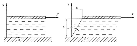
Fluid mechanics is concerned with the behavior of materials which deform without limit under the influence of shearing forces. Even a very small shearing force will deform a fluid body, but the velocity of the deformation will be correspondingly small. This property serves as the definition of a fluid: the shearing forces necessary to deform a fluid body go to zero as the velocity of deformation tends to zero. On the contrary, the behavior of a solid body is such that the deformation itself, not the velocity of deformation, goes to zero when the forces necessary to deform it tend to zero. To illustrate this contrasting behavior, consider a material between two parallel plates and adhering to them acted on by a shearing force $F$ (Fig. 1.1).
If the extent of the material in the direction normal to the plane of Fig. 1.1 and in the $x$-direction is much larger than that in the $y$-direction, experience shows that for many solids (Hooke’s solids), the force per unit area $\tau=F / A$ is proportional to the displacement $a$ and inversely proportional to the distance between the plates $h$. At least one dimensional quantity typical for the material must enter this relation, and here this is the shear modulus $G$. The relationship $$ \tau=G \gamma(\gamma \ll 1) $$ between the shearing angle $\gamma=a / h$ and $\tau$ satisfies the definition of a solid: the force per unit area $\tau$ tends to zero only when the deformation $\gamma$ itself goes to zero. Often the relation for a solid body is of a more general form, e.g., $\tau=f(\gamma)$, with $f(0)=0$. If the material is a fluid, the displacement of the plate increases continually with time under a constant shearing force. This means there is no relationship between the displacement, or deformation, and the force. Experience shows here that with many fluids the force is proportional to the rate of change of the displacement, that is, to the velocity of the deformation. Again the force is inversely proportional to the distance between the plates. (We assume that the plate is being dragged at
constant speed, so that the inertia of the material does not come into play.) The dimensional quantity required is the shear viscosity $\eta$, and the relationship with $U=\mathrm{d} a / \mathrm{d} t$ now reads $$ \tau=\eta \frac{U}{h}=\eta \dot{\gamma}, $$ or, if the shear rate $\dot{\gamma}$ is set equal to $\mathrm{d} u / \mathrm{d} y$. $$ \tau(y)=\eta \frac{\mathrm{d} u}{\mathrm{~d} y} . $$ $\tau(y)$ is the shêar streess on a surfacee eelement parallèl to the plates at point $y$. In so-called simple shearing flow (rectilinear shearing flow) only the $x$-component of the velocity is nonzero, and is a linear function of $y$.
The above relationship was known to Newton, and it is sometimes incorrectly used as the definition of a Newtonian fluid: there are also non-Newtonian fluids which show a linear relationship between the shear stress $\tau$ and the shear rate $\dot{\gamma}$ in this simple state of stress. In general, the relationship for a fluid reads $\tau=f(\dot{\gamma})$, with $f(0)=0$.
While there are many substances for which this classification criterion suffices, there are some which show dual character. These include the glasslike materials which do not have a crystal structure and are structurally liquids. Under prolonged loads these substances begin to flow, that is to deform without limit. Under short-term loads, they exhibit the behavior of a solid body. Asphalt is an oftquoted example: you can walk on asphalt without leaving footprints (short-term load), but if you remain standing on it for a long time, you will finally sink in. Under very short-term loads, e.g., a blow with a hammer, asphalt splinters, revealing its structural relationship to glass. Other materials behave like solids even in the long-term, provided they are kept below a certain shear stress, and then above this stress they will behave like liquids. A typical example of these substances (Bingham materials) is paint: it is this behavior which enables a coat of paint to stick to surfaces parallel to the force of gravity.
物理代写|流体力学代写Fluid Mechanics代考|The behavior of solids
The behavior of solids, liquids and gases described up to now can be explained by the molecular structure, by the thermal motion of the molecules, and by the interactions between the molecules. Microscopically the main difference between gases on the one hand, and liquids and solids on the other is the mean distance between the molecules.
With gases, the spacing at standard temperature and pressure $(273.2 \mathrm{~K}$; $1.013$ bar) is about ten effective molecular diameters. Apart from occasional collisions, the molecules move along a straight path. Only during the collision of, as a rule, two molecules, does an interaction take place. The molecules first attract each other weakly, and then as the interval between them becomes noticeably smaller than the effective diameter, they repel strongly. The mean free path is in general larger than the mean distance, and can occasionally be considerably larger.
With liquids and solids the mean distance is about one effective molecular diameter. In this case there is always an interaction between the molecules. The large resistance which liquids and solids show to volume changes is explained by the repulsive force between molecules when the spacing becomes noticeably smaller than their effective diameter. Even gases have a resistance to change in volume, although at standard temperature and pressure it is much smaller and is proportional to the kinetic energy of the molecules. When the gas is compressed so far that the spacing is comparable to that in a liquid, the resistance to volume change becomes large, for the same reason as referred to above.
Real solids show a crystal structure: the molecules are arranged in a lattice and vibrate about their equilibrium position. Above the melting point, this lattice disintegrates and the material becomes liquid. Now the molecules are still more or less ordered, and continue to carry out their oscillatory motions although they often exchange places. The high mobility of the molecules explains why it is easy to deform liquids with shearing forces.
It would appear obvious to describe the motion of the material by integrating the equations of motion for the molecules of which it consists: for computational reasons this procedure is impossible since in general the number of molecules in the material is very large. But it is impossible in principle anyway, since the position and momentum of a molecule cannot be simultaneously known (Heisenberg’s Uncertainty Principle) and thus the initial conditions for the integration do not exist. $\mathrm{~ I n ~ a ̊ d d i t i o ̄ n , ~ d e t a ̄ i l e ̉ ~ i n f o r m a ̄ t i o n ̃ ~ a b o o u t ~ t h e ~ m o ̄ l e ́ c u l a}$ and therefore it would be necessary to average the molecular properties of the motion in some suitable way. It is therefore far more appropriate to consider the average properties of a cluster of molecules right from the start.
物理代写|流体力学代写Fluid Mechanics代考|On the other hand the linear measure of the volume
On the other hand the linear measure of the volume must be small compared to the macroscopic length of interest. It is appropriate to assume that the volume of the fluid particle is infinitely small compared to the whole volume occupied by the fluid. This assumption forms the basis of the continuum hypothesis. Under this hypothesis we consider the fluid particle to be a material point and the density (or other properties) of the fluid to be continuous functions of place and time. Occasionally we will have to relax this assumption on certain curves or surfaces, since discontinuities in the density or temperature, say, may occur in the context of some idealizations. The part of the fluid under observation consists then of infinitely many material points, and we expect that the motion of this continuum will be described by partial differential equations. However the assumptions which have led us from the material to the idealized model of the continuum are not always fulfilled. One example is the flow past a space craft at very high altitudes, where the air density is very low. The number of molecules required to do any useful averaging then takes up such a large volume that it is comparable to the volume of the craft itself.
Continuum theory is also inadequate to describe the structure of a shock (see Chap. 9), a frequent occurrence in compressible flow. Shocks have thicknesses of the same order of magnitude as the mean free path, so that the linear measures of the volumes required for averaging are comparable to the thickness of the shock. We have not yet considered the role the thermal motion of molecules plays in the continuum model. This thermal motion is reflected in the macroscopic properties of the material and is the single source of viscosity in gases. Even if the macroscopic velocity given by (1.4) is zero, the molecular velocities $\vec{c}{i}$ are clearly not necessarily zero. The consequence of this is that the molecules migrate out of the fluid particle and are replaced by molecules drifting in. This exchange process gives rise to the macroscopic fluid properties called transport properties. Obviously, molecules with other molecular properties (e.g. mass) are brought into the fluid particle. Take as an example a gas which consists of two types of molecule, say $\mathrm{O}{2}$ and $\mathrm{N}{2}$. Let the number of $\mathrm{O}{2}$ molecules per unit volume in the fluid particle be larger than that of the surroundings. The number of $\mathrm{O}_{2}$ molecules which migrate out is proportional to the number density inside the fluid particle, while the number which drift in is proportional to that of the surroundings. The net effect is that more $\mathrm{O}{2}$ molecules drift in than drift out and so the $\mathrm{O}{2}$ number density adjusts itself to the surroundings. From the standpoint of continuum theory the process described above represents the diffusion.
物理代写|流体力学代写Fluid Mechanics代考|The Concept of the Continuum and Kinematics