多尺度模型代写Multilevel Models代考2023
如果你也在多尺度模型Multilevel Models这个学科遇到相关的难题,请随时添加vx号联系我们的代写客服。我们会为你提供专业的服务。
statistics-lab™ 长期致力于留学生网课服务,涵盖各个网络学科课程:金融学Finance,经济学Economics,数学Mathematics,会计Accounting,文学Literature,艺术Arts等等。除了网课全程托管外,statistics-lab™ 也可接受单独网课任务。无论遇到了什么网课困难,都能帮你完美解决!
statistics-lab™ 为您的留学生涯保驾护航 在代写代考多尺度模型Multilevel Models方面已经树立了自己的口碑, 保证靠谱, 高质量且原创的统计Statistics和数学Math代写服务。我们的专家在代考多尺度模型Multilevel Models相关的作业也就用不着说。
多尺度模型代写Multilevel Models代考
多层次模型(MLM),又称层次线性模型(HLM)、线性混合效应模型、混合模型、嵌套数据模型、随机系数模型、随机效应模型、随机参数模型、拆分模型。 也称小区设计,是一种参数在多个层次上变化的统计模型。 由学生个人成绩和学生所属班级成绩组成的学生成绩模型就是一个例子。 它可以看作是线性模型(特别是线性回归)的一般化,但也可以扩展到非线性模型。 自从有了足够的计算能力和软件之后,这些模型变得越来越普遍。
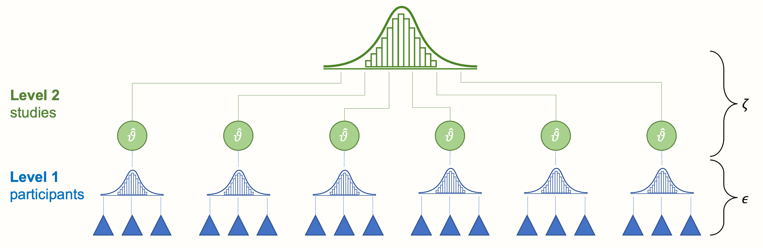
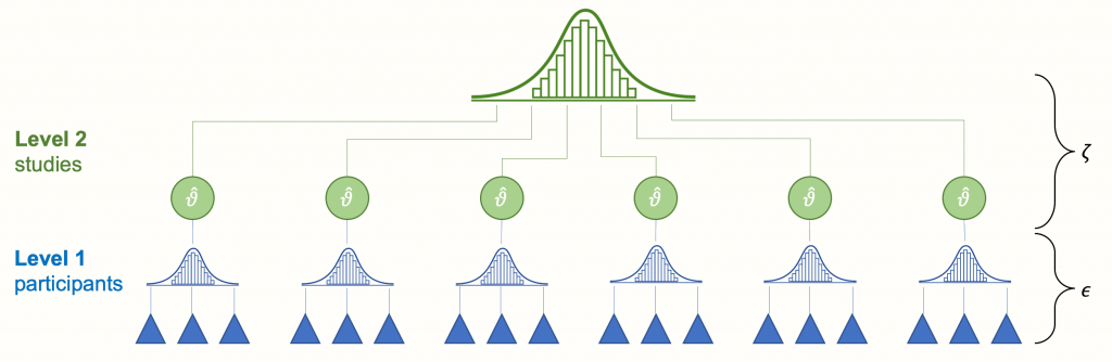
多层次模型特别适用于将参与者数据分为多个层次(嵌套数据)的研究设计。 分析单位通常是个人(较低层次),嵌套在上下文和集体单位(较高层次)中。 多层次模型的最低层次通常是个体,但也可以对个体进行重复测量。 因此,多层次模型为重复测量的单变量或多变量分析提供了另一种选择。 可以研究生长曲线的个体差异。 此外,多层次模型还可用作方差分析的替代方法,即在根据协变量(如个体差异)调整因变量得分后,检验处理方法的差异。 多层次模型可以分析这些实验,而无需假设协方差分析所要求的回归系数的一致性。
虽然多层次模型可以应用于多层次数据,但本文将只讨论最常见的两层模型。 因变量需要在最低的分析层次上考虑。
多尺度模型Multilevel Models包含几个不同的主题,列举如下:
随机截距模型Random Intercept Model代写代考
随机截距模型是一种允许截距在组间变化的模型。 该模型假定斜率在各组间是恒定的。 此外,该模型还提供了类内相关性的信息。 这有助于确定是否首先需要多层次模型。
随机斜率模型Random Slope Model代写代考
随机斜率模型是一种允许斜率变化的模型;在这种模型中,不同组间的斜率不同,但假定不同组间的截距不变。
其他相关科目课程代写:
- 广义线性模型Generalized linear model
- 广义线性混合模型 Generalized linear mixed model
- 贝叶斯分层模型Bayesian hierarchical modeling
多尺度模型Multilevel Models分析手法
分析分层数据的方法有几种,其中大多数都存在问题。
首先,根据传统的统计方法,可以将高阶变量分解为个体层次,并在个体层次上进行分析(为每个个体分配类变量)。 这种方法的问题在于它违反了独立性假设,可能会使结果产生偏差。 这就是所谓的原子谬误。
传统统计方法的另一种可行替代方法是将个体层面的变量汇总为高阶变量,并在高阶变量上进行分析。 在这种方法中,由于取的是个体变量的平均值,组内的所有信息都被丢弃了;多达 80-90% 的方差被浪费掉了,汇总变量之间的关系被夸大,从而被扭曲。 这就是所谓的生态谬误,从统计学角度看,会导致信息丢失和能力下降。
另一种分析分层数据的方法是使用随机系数模型。 该模型假定每个组都有一个不同的回归模型,每个模型都有自己的截距和斜率。 由于分组是抽样的,该模型还假设截距和斜率是从分组截距和斜率群体中随机抽取的。 这样,分析就可以假设斜率是固定的,但截距可以变化。 然而,这样做也有问题。 这是因为个体成分和独立成分是独立的,而群体成分只是群体之间独立,群体内部依存。 也可以分析斜率是随机的,但误差项的相关性取决于个体水平变量的值。 因此,使用随机系数模型分析层次数据的问题在于无法纳入高阶变量。
There are several ways to analyse stratified data, most of which are problematic.
First, according to traditional statistical methods, higher order variables can be decomposed into individual levels and analysed at the individual level (assigning class variables to each individual). The problem with this approach is that it violates the assumption of independence and may bias the results. This is known as the atomic fallacy.
Another viable alternative to the traditional statistical approach is to aggregate the individual level variables into higher order variables and analyse them at the higher order variables. In this approach, all information within the group is discarded as the average of the individual variables is taken; up to 80-90% of the variance is wasted, and the relationships between the aggregated variables are exaggerated and thus distorted. This is known as the ecological fallacy and statistically leads to lost information and reduced power.
Another way to analyse stratified data is to use a random coefficient model. This model assumes that each group has a different regression model, each with its own intercept and slope. Since the groups are sampled, the model also assumes that the intercepts and slopes are randomly drawn from the grouped intercept and slope populations. In this way, the analysis can assume that the slopes are fixed, but the intercepts can vary. However, there are problems with this. This is because the individual and independent components are independent, whereas the group components are only independent between groups and dependent within groups. It is also possible to analyse the slope as random, but the correlation of the error term depends on the value of the individual level variable. The problem with using a random coefficient model to analyse hierarchical data is therefore the inability to incorporate higher order variables.

统计代写请认准statistics-lab™. statistics-lab™为您的留学生涯保驾护航。
多尺度模型Multilevel Models的重难点
什么是第 1 级回归方程Level 1 regression equation?
如果第 1 层有一个自变量,则第 1 层模型如下。
$$
Y_{i j}=\beta_{0 j}+\beta_{1 j} X_{i j}+e_{i j}
$$
$$Y_{i j}$$ – 每个观察值在第 1 层的因变量得分,其中 i 是个案,j 是组。
- $X_{i j}$$-第 1 层的预测因子
- $\beta_{0 j}$-因变量在第 j 组的截距(第 2 层)
$\beta_{1 j}$- 因变量 $Y_{i j}$ 与第 1 层预测因子 $X_{i j}$ 在第 j 组(第 2 层)之间的斜率
▪ $E_{i j}$-预测第 1 层方程的随机误差 $\left(r_{i j}\right.$)
第 1 级假设一组内的截距和斜率要么没有变化(现实中很少见),要么是非随机变化(可从第 2 级自变量中预测),要么是随机变化(有自己的总体分布)[2]。
如果存在多个一级自变量,则可以通过将向量或矩阵代入方程来扩展模型。
如果响应 $Y_{i j}$ 与预测变量 $X_{i j}$ 之间的关系是非线性的,则可以用非线性函数来表示这种关系,从而将模型扩展为非线性混合效应模型。 例如,如果响应 $Y_{i j}$ 代表第 i 个国家的累积感染轨迹,而 $X_{i j}$ 代表第 j 个时间点,则每个国家的有序对 $\left(X_{i j}, Y_{i j}\right)$ 的形式可能类似于 logistic 函数。
什么是开发多层次模型Developing multi-level models?
要进行多层次模型分析,应从固定系数(截距和斜率)开始。 每次只能改变一个方面,并与之前的模型进行比较。 当研究人员评估一个模型时,他们会检查三件事。 第一,它是一个好模型吗? 第二,更复杂的模型是否更好? 第三,各个预测因子对模型有什么贡献?
为了评估一个模型,需要检查各种模型拟合统计量[2]。 其中一种统计量是卡方似然比检验,用于评估模型之间的差异。 似然比检验可用于一般模型的建立、检验模型中的效应变化时的情况、将虚拟代码分类变量作为单一效应进行检验等。 然而,只有当模型是嵌套的(一个更复杂的模型包括一个更简单模型的所有效应)时,才能使用这种检验。 在测试非嵌套模型时,可以使用 Akaike 信息准则(AIC)或贝叶斯信息准则(BIC)对模型进行比较。
什么是2级回归方程Level 2 regression equation?
图形着色是为图形中的某些元素分配颜色,使其满足某些约束条件。 最简单地说,就是给所有顶点着色,使相邻顶点不具有相同颜色。 这就是顶点着色。 同样,边着色是给所有边着色,使相邻边不具有相同颜色的问题;面着色是给平面图中边所围成的每个区域(面)着色,使相邻面不具有相同颜色的问题。
因变量是㧍到第 2 级组的第 1 级自变量的截距和斜率。
$$
\begin{aligned}
& \beta_{0 j}=\gamma_{00}+\gamma_{01} W_j+u_{0 j} \
& \beta_{1 j}=\gamma_{10}+u_{1 j}
\end{aligned}
$$
$\gamma_{00}$ -总截距(当所有预测因子等于 0 时,所有组的因变量得分平均值)
- $W_j$ – 二级预测因子。
- $\gamma_{01}$ – 因变量 $\beta_{1 j}$与二级预测因子 $W_j$ 之间的总体回归系数(斜率
- $u_{0 j}$- 组截距与总体截距之差的随机误差
- $\gamma_{10}$ – 因变量$\beta_{1 j}$ 与第 1 层预测因子$X_{i j}$ 之间的总体回归系数(斜率
- $u_{1 j}$斜率的误差成分${ }^{[2]}$(总体斜率与组斜率之差)
多尺度模型Multilevel Models的相关课后作业范例
这是一篇关于图论Graph Theoryry的作业
This box summarizes the terminology for the various algebraic terms used in the models i
$y_{i j}$ is the dependent variable: the outcome for individual $i$ living in neighbourhood $j$. Individuals are numbered from $i=1, \ldots, N$ and each lives in one neighbourhood $j=1, \ldots, J$. There are $n_j$ individuals from neighbourhood $j$ so $N=\sum_{j=1}^J n_j$.
$x_{p i j}$ are the independent variables, measured on individual $i$ in neighbourhood $j$. The subscript $p$ is used to distinguish between the variables.
$x_{p j}$ are independent variables, measured at the neighbourhood level; this variable takes the same value for all individuals living in neighbourhood $j$.
$\beta_0$ is used to denote the intercept.
$\beta_p$ is the regression coefficient associated with $x_{p i j}$ or $x_{p j}$.
$u_{0 j}$ is the estimated effect or residual for area $j$. This is the difference in the outcome for an individual in neighbourhood $j$ compared to an individual in the average neighbourhood, after taking into account those characteristics that have been included in the model. The 0 in the subscript denotes that this is a random intercept residual, a departure from the overall intercept $\beta_0$ applying equally to everyone in neighbourhood $j$ regardless of individual characteristics.
$u_{p j}$ is the slope residual for neighbourhood $j$ that is associated with the independent variable $x_{p i j}$ or $x_{p j}$. Just as $u_{0 j}$ denotes a departure from the overall intercept $\beta_0, u_{p j}$ indicates the extent of a departure from the overall slope in a random slope model.
$e_{0 i j}$ is the individual-level residual or error term for individual $i$ in neighbourhood $j$.
$\sigma_{u 0}^2$ is the| variance of the neighbourhood-level intercept residuals $u_{0 j}$.
$\sigma_{u p}^2$ is the variance of the neighbourhood-level slope residuals $u_{p j}$.
$\sigma_{u 0 p}$ is the covariance between the neighbourhood-level intercept residuals $u_{0 j}$ and slope residuals $u_{p j}$.
$\sigma_{e 0}^2$ is the variance of the individual-level errors $e_{0 i j}$.
$\rho_{\mathrm{I}}$ is the intraclass correlation coefficient or the proportion of the total variation in the outcome that is attributable to differences between areas.
最后的总结:
通过对多尺度模型Multilevel Models各方面的介绍,想必您对这门课有了初步的认识。如果你仍然不确定或对这方面感到困难,你仍然可以依靠我们的代写和辅导服务。我们拥有各个领域、具有丰富经验的专家。他们将保证你的 essay、assignment或者作业都完全符合要求、100%原创、无抄袭、并一定能获得高分。需要如何学术帮助的话,随时联系我们的客服。