标签: ENG 4063

数学代写|信息论代写information theory代考|The Relationship Between Logical Entropy and Shannon Entropy

如果你也在 怎样代写信息论information theory这个学科遇到相关的难题,请随时右上角联系我们的24/7代写客服。

信息论是对数字信息的量化、存储和通信的科学研究。该领域从根本上是由哈里-奈奎斯特和拉尔夫-哈特利在20世纪20年代以及克劳德-香农在20世纪40年代的作品所确立的。

statistics-lab™ 为您的留学生涯保驾护航 在代写信息论information theory方面已经树立了自己的口碑, 保证靠谱, 高质且原创的统计Statistics代写服务。我们的专家在代写信息论information theory代写方面经验极为丰富,各种代写信息论information theory相关的作业也就用不着说。

我们提供的信息论information theory及其相关学科的代写,服务范围广, 其中包括但不限于:

  • Statistical Inference 统计推断
  • Statistical Computing 统计计算
  • Advanced Probability Theory 高等概率论
  • Advanced Mathematical Statistics 高等数理统计学
  • (Generalized) Linear Models 广义线性模型
  • Statistical Machine Learning 统计机器学习
  • Longitudinal Data Analysis 纵向数据分析
  • Foundations of Data Science 数据科学基础
数学代写|信息论代写information theory代考|The Relationship Between Logical Entropy and Shannon Entropy

数学代写|信息论代写information theory代考|Brief History of the Logical Entropy Formula

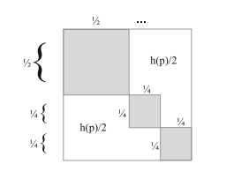
The logical entropy formula $h(p)=\sum_{i} p_{i}\left(1-p_{i}\right)=1-\sum_{i} p_{i}^{2}$ is the probability of getting distinct values $u_{i} \neq u_{j}$ in two independent samplings of the random variable $u$. The complementary measure $1-h(p)=\sum_{i} p_{i}^{2}$ is the probability that the two drawings yield the same value from $U$. Thus $1-\sum_{i} p_{i}^{2}$ is a measure of heterogeneity or diversity in keeping with our theme of information as distinctions, while the complementary measure $\sum_{i} p_{i}^{2}$ is a measure of homogeneity or concentration. Historically, the formula can be found in either form depending on the particular context. The $p_{i}$ ‘s might be relative shares such as the relative share of organisms of the $i$ th species in some population of organisms, and then

the interpretation of $p_{i}$ as a probability arises by considering the random choice of an organism from the population.

According to I. J. Good, the formula has a certain naturalness: “If $p_{1}, \ldots, p_{t}$ are the probabilities of $t$ mutually exclusive and exhaustive events, any statistician of this century who wanted a measure of homogeneity would have take about two seconds to suggest $\sum p_{i}^{2}$ which I shall call $\rho . “[13$, p. 561] As noted by Bhargava and Uppuluri [4], the formula $1-\sum p_{i}^{2}$ was used by Gini in 1912 [10] as a measure of “mutability” or diversity. But another development of the formula (in the complementary form) in the early twentieth century was in cryptography. The American cryptologist, William F. Friedman, devoted a 1922 book [9] to the “index of coincidence” (i.e., $\sum p_{i}^{2}$ ). Solomon Kullback (see the Kullback-Leibler divergence treated later) worked as an assistant to Friedman and wrote a book on cryptology which used the index [16].

During World War II, Alan M. Turing worked for a time in the Government Code and Cypher School at the Bletchley Park facility in England. Probably unaware of the earlier work, Turing used $\rho=\sum p_{i}^{2}$ in his cryptoanalysis work and called it the repeat rate since it is the probability of a repeat in a pair of independent draws from a population with those probabilities (i.e., the identification probability $1-h(p)$ ). Polish cryptoanalysts had independently used the repeat rate in their work on the Enigma [21].

数学代写|信息论代写information theory代考|Shannon Entropy

For a partition $\pi=\left{B_{1}, \ldots, B_{m}\right}$ with block probabilities $p\left(B_{i}\right)$ (obtained using equiprobable points or with point probabilities), the Shannon entropy of the partition (using logs to base 2) is:
$$
H(\pi)=-\sum_{i=1}^{m} p\left(B_{i}\right) \log \left(p\left(B_{i}\right)\right)
$$
Or if given a finite probability distribution $p=\left{p_{1}, \ldots, p_{m}\right}$, the Shannon entropy of the probability distribution is:
$$
H(p)=-\sum_{i=1}^{m} p_{i} \log \left(p_{i}\right)
$$
The Shannon entropy is often presented as being the same as the Boltzmann entropy $S=\frac{1}{n} \ln \left(\frac{n !}{n_{1} ! \ldots n_{m} !}\right)$; it is even called the “Shannon-Boltzmann entropy” by

many authors. The story is that when presented with Shannon’s formula, John von Neumann suggested calling it “entropy” since it occurs in statistical mechanicsand since Shannon could always win arguments since no one really knows what entropy is. But it only occurs in statistical mechanics as a numerical approximation based on taking the first two terms in the Stirling approximation formula for $\ln (n !)$. The first two terms in the Stirling approximation for $\ln (N !)$ are: $\ln (N !) \approx$ $N \ln (N)-N$

If we consider a partition on a finite $U$ with $|U|=N$, with $n$ blocks of size $N_{1}, \ldots, N_{n}$, then the number of ways of distributing the individuals in these $n$ boxes with those numbers $N_{i}$ in the $i$ th box is: $W=\frac{N !}{N_{1} ! \times \ldots \times N_{n} !}$. The normalized natural $\log$ of $W, S=\frac{1}{N} \ln (W)$ is one form of entropy in statistical mechanics. Indeed, the formula $S=k \log (W)$ is engraved on Boltzmann’s tombstone.

The entropy formula can then be developed using the first two terms in the Stirling approximation.
$$
\begin{gathered}
S=\frac{1}{N} \ln (W)=\frac{1}{N} \ln \left(\frac{N !}{N_{1} ! \times \ldots \times N_{n} !}\right)=\frac{1}{N}\left[\ln (N !)-\sum_{i} \ln \left(N_{i} !\right)\right] \
\approx \frac{1}{N}\left[N[\ln (N)-1]-\sum_{i} N_{i}\left[\ln \left(N_{i}\right)-1\right]\right] \
=\frac{1}{N}\left[N \ln (N)-\sum N_{i} \ln \left(N_{i}\right)\right]=\frac{1}{N}\left[\sum N_{i} \ln (N)-\sum N_{i} \ln \left(N_{i}\right)\right] \
=\sum \frac{N_{i}}{N} \ln \left(\frac{1}{N_{i} / N}\right)=\sum p_{i} \ln \left(\frac{1}{p_{i}}\right)=H_{e}(p)
\end{gathered}
$$

数学代写|信息论代写information theory代考|Logical Entropy, Not Shannon Entropy

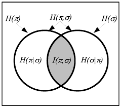
Shannon entropy and the many other suggested ‘entropies’ (Rényi, Tsallis, etc.) are routinely called “measures” of information in the general sense of a real-valued quantification -but not in the sense of measure theory. The formulas for mutual information, joint entropy, and conditional entropy are defined so these Shannon entropies satisfy Venn diagram formulas. As Lorne Campbell put it:
Certain analogies between entropy and measure have been noted by various authors. These analogies provide a convenient mnemonic for the various relations between entropy, conditional entropy, joint entropy, and mutual information. It is interesting to speculate whether these analogies have a deeper foundation. It would seem to be quite significant if entropy did admit an interpretation as the measure of some set. [1, p. 112]

For any finite set $U$, a measure $\mu$ is a function $\mu: \wp(U) \rightarrow \mathbb{R}$ such that:

  1. $\mu(\emptyset)=0$,
  2. for any $E \subseteq U, \mu(E) \geq 0$, and
  3. for any disjoint subsets $E_{1}$ and $E_{2}, \mu\left(E_{1} \cup E_{2}\right)=\mu\left(E_{1}\right)+\mu\left(E_{2}\right)$.
    The standard usage in measure theory $[4,3]$ seems to be that a “measure” is defined to be non-negative, and the extension to allow negative values is a “signed measure.” That definition is used here although a few authors [10] define a measure to allow negative values and then call the restriction to non-negative values a “positive measure.” The point to notice is that both measures and signed measures can be represented as Venn diagrams (allowing negative areas). As we will see, for three or more random variables, the Shannon mutual information can have negative values-which has no known interpretation. But there is an interesting difference. The logical entropies are defined in terms of a probability measure on a set. The compound Shannon entropies are defined ‘directly’ so as to satisfy the Venn diagram relationships without any mention of a set on which the Venn diagram is defined. As one author put it: “Shannon carefully contrived for this ‘accident’ to occur” [11, p. 153]. But it is possible ex post to then define a set so that the alreadydefined Shannon entropies are the appropriate values on subsets of that set. The ex post construction for the Shannon entropies was first carried out by Kuo Ting Hu [6] but was also noted by Imre Csiszar and Janos Körner [2], and redeveloped by Raymond Yeung [14]. Outside the context of Shannon entropies, the underlying mathematical facts about additive set functions and the inclusion-exclusion principle were known at least from the 1925 first edition of the Polya-Szego classic [9] and Ryser’s treatment of combinatorics [12]-all well-developed in [13].
数学代写|信息论代写information theory代考|The Relationship Between Logical Entropy and Shannon Entropy

信息论代考

数学代写|信息论代写information theory代考|Brief History of the Logical Entropy Formula

逻辑熵公式H(p)=∑一世p一世(1−p一世)=1−∑一世p一世2是获得不同值的概率在一世≠在j在随机变量的两个独立抽样中在. 补充措施1−H(p)=∑一世p一世2是两张图产生相同值的概率在. 因此1−∑一世p一世2是异质性或多样性的衡量标准,与我们将信息作为区分的主题保持一致,而补充衡量标准∑一世p一世2是均匀性或浓度的量度。从历史上看,这个公式可以根据特定的上下文以任何一种形式出现。这p一世的可能是相对份额,例如生物体的相对份额一世某些生物种群中的第 th 种,然后

的解释p一世因为概率是通过考虑从种群中随机选择一个有机体而产生的。

根据 IJ Good 的说法,该公式具有一定的自然性:“如果p1,…,p吨是概率吨相互排斥和详尽的事件,本世纪任何想要衡量同质性的统计学家都需要大约两秒钟的时间来提出建议∑p一世2我称之为ρ.“[13,页。561] 正如 Bhargava 和 Uppuluri [4] 所指出的,公式1−∑p一世2Gini 在 1912 年 [10] 使用它来衡量“可变性”或多样性。但在 20 世纪初,该公式(以互补形式)的另一个发展是在密码学中。美国密码学家威廉·弗里德曼 (William F. Friedman) 在 1922 年的一本书 [9] 中专门讨论了“巧合指数”(即,∑p一世2)。Solomon Kullback(参见稍后处理的 Kullback-Leibler 散度)担任弗里德曼的助手,并写了一本使用索引的密码学书籍 [16]。

二战期间,艾伦 M. 图灵曾在英国布莱切利公园设施的政府密码和密码学校工作过一段时间。可能不知道早期的工作,图灵使用ρ=∑p一世2在他的密码分析工作中,将其称为重复率,因为它是具有这些概率的群体中一对独立抽取中重复的概率(即识别概率1−H(p))。波兰密码分析家在他们的 Enigma [21] 工作中独立使用了重复率。

数学代写|信息论代写information theory代考|Shannon Entropy

对于一个分区\pi=\left{B_{1}, \ldots, B_{m}\right}\pi=\left{B_{1}, \ldots, B_{m}\right}有块概率p(乙一世)(使用等概率点或点概率获得),分区的香农熵(使用以 2 为底的对数)为:

H(圆周率)=−∑一世=1米p(乙一世)日志⁡(p(乙一世))
或者如果给定一个有限的概率分布p=\left{p_{1}, \ldots, p_{m}\right}p=\left{p_{1}, \ldots, p_{m}\right},概率分布的香农熵为:

H(p)=−∑一世=1米p一世日志⁡(p一世)
香农熵通常与玻尔兹曼熵相同小号=1nln⁡(n!n1!…n米!); 它甚至被称为“香农-玻尔兹曼熵”

许多作者。故事是,当提出香农公式时,约翰·冯·诺依曼建议称其为“熵”,因为它出现在统计力学中,而且香农总是能赢得争论,因为没有人真正知道熵是什么。但它只出现在统计力学中,作为基于斯特林近似公式中前两项的数值近似ln⁡(n!). 斯特林近似中的前两项ln⁡(ñ!)是:ln⁡(ñ!)≈ ñln⁡(ñ)−ñ

如果我们考虑一个有限的分区在和|在|=ñ, 和n大小块ñ1,…,ñn,那么这些个体的分布方式的数量n带有这些数字的盒子ñ一世在里面一世第一个盒子是:在=ñ!ñ1!×…×ñn!. 归一化的自然日志的在,小号=1ñln⁡(在)是统计力学中熵的一种形式。确实,公式小号=ķ日志⁡(在)刻在玻尔兹曼的墓碑上。

然后可以使用斯特林近似中的前两项来开发熵公式。

小号=1ñln⁡(在)=1ñln⁡(ñ!ñ1!×…×ñn!)=1ñ[ln⁡(ñ!)−∑一世ln⁡(ñ一世!)] ≈1ñ[ñ[ln⁡(ñ)−1]−∑一世ñ一世[ln⁡(ñ一世)−1]] =1ñ[ñln⁡(ñ)−∑ñ一世ln⁡(ñ一世)]=1ñ[∑ñ一世ln⁡(ñ)−∑ñ一世ln⁡(ñ一世)] =∑ñ一世ñln⁡(1ñ一世/ñ)=∑p一世ln⁡(1p一世)=H和(p)

数学代写|信息论代写information theory代考|Logical Entropy, Not Shannon Entropy

香农熵和许多其他建议的“熵”(Rényi、Tsallis 等)通常在实值量化的一般意义上被称为信息的“测量”——但不是在测量理论的意义上。定义了互信息、联合熵和条件熵的公式,因此这些香农熵满足维恩图公式。正如 Lorne Campbell 所说:
熵和度量之间的某些类比已被许多作者注意到。这些类比为熵、条件熵、联合熵和互信息之间的各种关系提供了方便的助记符。推测这些类比是否有更深的基础是很有趣的。如果熵确实允许将解释解释为某些集合的度量,那似乎是非常重要的。[1,第 112]

对于任何有限集在, 一种方法μ是一个函数μ:℘(在)→R这样:

  1. μ(∅)=0,
  2. 对于任何和⊆在,μ(和)≥0, 和
  3. 对于任何不相交的子集和1和和2,μ(和1∪和2)=μ(和1)+μ(和2).
    测度论中的标准用法[4,3]似乎“度量”被定义为非负数,而允许负值的扩展是“有符号度量”。尽管一些作者 [10] 定义了一个允许负值的度量,然后将对非负值的限制称为“正度量”,但这里使用了该定义。需要注意的一点是,度量和签名度量都可以表示为维恩图(允许负区域)。正如我们将看到的,对于三个或更多随机变量,香农互信息可以具有负值——这没有已知的解释。但是有一个有趣的区别。逻辑熵是根据集合上的概率度量来定义的。复合香农熵被“直接”定义以满足维恩图关系,而无需提及定义维恩图的集合。正如一位作者所说:“香农精心设计了这个‘意外’的发生”[11, p. 153]。但是可以事后定义一个集合,以便已经定义的香农熵是该集合子集上的适当值。香农熵的事后构造首先由 Kuo Ting Hu [6] 进行,但 Imre Csiszar 和 Janos Körner [2] 也注意到了这一点,并由 Raymond Yeung [14] 重新开发。在香农熵的范围之外,关于加法集函数和包含-排除原理的基本数学事实至少从 1925 年第一版的 Polya-Szego 经典 [9] 和 Ryser 对组合学的处理 [12] 中得知——一切都很好-在[13]中开发。但是可以事后定义一个集合,以便已经定义的香农熵是该集合子集上的适当值。香农熵的事后构造首先由 Kuo Ting Hu [6] 进行,但 Imre Csiszar 和 Janos Körner [2] 也注意到了这一点,并由 Raymond Yeung [14] 重新开发。在香农熵的范围之外,关于加法集函数和包含-排除原理的基本数学事实至少从 1925 年第一版的 Polya-Szego 经典 [9] 和 Ryser 对组合学的处理 [12] 中得知——一切都很好-在[13]中开发。但是可以事后定义一个集合,以便已经定义的香农熵是该集合子集上的适当值。香农熵的事后构造首先由 Kuo Ting Hu [6] 进行,但 Imre Csiszar 和 Janos Körner [2] 也注意到了这一点,并由 Raymond Yeung [14] 重新开发。在香农熵的范围之外,关于加法集函数和包含-排除原理的基本数学事实至少从 1925 年第一版的 Polya-Szego 经典 [9] 和 Ryser 对组合学的处理 [12] 中得知——一切都很好-在[13]中开发。香农熵的事后构造首先由 Kuo Ting Hu [6] 进行,但 Imre Csiszar 和 Janos Körner [2] 也注意到了这一点,并由 Raymond Yeung [14] 重新开发。在香农熵的范围之外,关于加法集函数和包含-排除原理的基本数学事实至少从 1925 年第一版的 Polya-Szego 经典 [9] 和 Ryser 对组合学的处理 [12] 中得知——一切都很好-在[13]中开发。香农熵的事后构造首先由 Kuo Ting Hu [6] 进行,但 Imre Csiszar 和 Janos Körner [2] 也注意到了这一点,并由 Raymond Yeung [14] 重新开发。在香农熵的范围之外,关于加法集函数和包含-排除原理的基本数学事实至少从 1925 年第一版的 Polya-Szego 经典 [9] 和 Ryser 对组合学的处理 [12] 中得知——一切都很好-在[13]中开发。
数学代写|信息论代写information theory代考 请认准statistics-lab™

统计代写请认准statistics-lab™. statistics-lab™为您的留学生涯保驾护航。

金融工程代写

金融工程是使用数学技术来解决金融问题。金融工程使用计算机科学、统计学、经济学和应用数学领域的工具和知识来解决当前的金融问题,以及设计新的和创新的金融产品。

非参数统计代写

非参数统计指的是一种统计方法,其中不假设数据来自于由少数参数决定的规定模型;这种模型的例子包括正态分布模型和线性回归模型。

广义线性模型代考

广义线性模型(GLM)归属统计学领域,是一种应用灵活的线性回归模型。该模型允许因变量的偏差分布有除了正态分布之外的其它分布。

术语 广义线性模型(GLM)通常是指给定连续和/或分类预测因素的连续响应变量的常规线性回归模型。它包括多元线性回归,以及方差分析和方差分析(仅含固定效应)。

有限元方法代写

有限元方法(FEM)是一种流行的方法,用于数值解决工程和数学建模中出现的微分方程。典型的问题领域包括结构分析、传热、流体流动、质量运输和电磁势等传统领域。

有限元是一种通用的数值方法,用于解决两个或三个空间变量的偏微分方程(即一些边界值问题)。为了解决一个问题,有限元将一个大系统细分为更小、更简单的部分,称为有限元。这是通过在空间维度上的特定空间离散化来实现的,它是通过构建对象的网格来实现的:用于求解的数值域,它有有限数量的点。边界值问题的有限元方法表述最终导致一个代数方程组。该方法在域上对未知函数进行逼近。[1] 然后将模拟这些有限元的简单方程组合成一个更大的方程系统,以模拟整个问题。然后,有限元通过变化微积分使相关的误差函数最小化来逼近一个解决方案。

tatistics-lab作为专业的留学生服务机构,多年来已为美国、英国、加拿大、澳洲等留学热门地的学生提供专业的学术服务,包括但不限于Essay代写,Assignment代写,Dissertation代写,Report代写,小组作业代写,Proposal代写,Paper代写,Presentation代写,计算机作业代写,论文修改和润色,网课代做,exam代考等等。写作范围涵盖高中,本科,研究生等海外留学全阶段,辐射金融,经济学,会计学,审计学,管理学等全球99%专业科目。写作团队既有专业英语母语作者,也有海外名校硕博留学生,每位写作老师都拥有过硬的语言能力,专业的学科背景和学术写作经验。我们承诺100%原创,100%专业,100%准时,100%满意。

随机分析代写


随机微积分是数学的一个分支,对随机过程进行操作。它允许为随机过程的积分定义一个关于随机过程的一致的积分理论。这个领域是由日本数学家伊藤清在第二次世界大战期间创建并开始的。

时间序列分析代写

随机过程,是依赖于参数的一组随机变量的全体,参数通常是时间。 随机变量是随机现象的数量表现,其时间序列是一组按照时间发生先后顺序进行排列的数据点序列。通常一组时间序列的时间间隔为一恒定值(如1秒,5分钟,12小时,7天,1年),因此时间序列可以作为离散时间数据进行分析处理。研究时间序列数据的意义在于现实中,往往需要研究某个事物其随时间发展变化的规律。这就需要通过研究该事物过去发展的历史记录,以得到其自身发展的规律。

回归分析代写

多元回归分析渐进(Multiple Regression Analysis Asymptotics)属于计量经济学领域,主要是一种数学上的统计分析方法,可以分析复杂情况下各影响因素的数学关系,在自然科学、社会和经济学等多个领域内应用广泛。

MATLAB代写

MATLAB 是一种用于技术计算的高性能语言。它将计算、可视化和编程集成在一个易于使用的环境中,其中问题和解决方案以熟悉的数学符号表示。典型用途包括:数学和计算算法开发建模、仿真和原型制作数据分析、探索和可视化科学和工程图形应用程序开发,包括图形用户界面构建MATLAB 是一个交互式系统,其基本数据元素是一个不需要维度的数组。这使您可以解决许多技术计算问题,尤其是那些具有矩阵和向量公式的问题,而只需用 C 或 Fortran 等标量非交互式语言编写程序所需的时间的一小部分。MATLAB 名称代表矩阵实验室。MATLAB 最初的编写目的是提供对由 LINPACK 和 EISPACK 项目开发的矩阵软件的轻松访问,这两个项目共同代表了矩阵计算软件的最新技术。MATLAB 经过多年的发展,得到了许多用户的投入。在大学环境中,它是数学、工程和科学入门和高级课程的标准教学工具。在工业领域,MATLAB 是高效研究、开发和分析的首选工具。MATLAB 具有一系列称为工具箱的特定于应用程序的解决方案。对于大多数 MATLAB 用户来说非常重要,工具箱允许您学习应用专业技术。工具箱是 MATLAB 函数(M 文件)的综合集合,可扩展 MATLAB 环境以解决特定类别的问题。可用工具箱的领域包括信号处理、控制系统、神经网络、模糊逻辑、小波、仿真等。

R语言代写问卷设计与分析代写
PYTHON代写回归分析与线性模型代写
MATLAB代写方差分析与试验设计代写
STATA代写机器学习/统计学习代写
SPSS代写计量经济学代写
EVIEWS代写时间序列分析代写
EXCEL代写深度学习代写
SQL代写各种数据建模与可视化代写

数学代写|信息论代写information theory代考|Logical Entropy

如果你也在 怎样代写信息论information theory这个学科遇到相关的难题,请随时右上角联系我们的24/7代写客服。

信息论是对数字信息的量化、存储和通信的科学研究。该领域从根本上是由哈里-奈奎斯特和拉尔夫-哈特利在20世纪20年代以及克劳德-香农在20世纪40年代的作品所确立的。

statistics-lab™ 为您的留学生涯保驾护航 在代写信息论information theory方面已经树立了自己的口碑, 保证靠谱, 高质且原创的统计Statistics代写服务。我们的专家在代写信息论information theory代写方面经验极为丰富,各种代写信息论information theory相关的作业也就用不着说。

我们提供的信息论information theory及其相关学科的代写,服务范围广, 其中包括但不限于:

  • Statistical Inference 统计推断
  • Statistical Computing 统计计算
  • Advanced Probability Theory 高等概率论
  • Advanced Mathematical Statistics 高等数理统计学
  • (Generalized) Linear Models 广义线性模型
  • Statistical Machine Learning 统计机器学习
  • Longitudinal Data Analysis 纵向数据分析
  • Foundations of Data Science 数据科学基础
数学代写|信息论代写information theory代考|Logical Entropy

数学代写|信息论代写information theory代考|Logical Information as the Measure of Distinctions

There is now a widespread view that information is fundamentally about differences, distinguishability, distinctions, and diversity. As Charles H. Bennett, one of the founders of quantum information theory, put it:

So information really is a very useful abstraction. It is the notion of distinguishability abstracted away from what we are distinguishing, or from the carrier of information. [3, p. 155$]$
This view even has an interesting history. In James Gleick’s book, The Information: A History, A Theory, A Flood, he noted the focus on differences in the seventeenth century polymath, John Wilkins, who was a founder of the Royal Society. In 1641 , the year before Isaac Newton was born, Wilkins published one of the earliest books on cryptography, Mercury or the Secret and Swift Messenger, which not only pointed out the fundamental role of differences but noted that any (finite) set of different things could be encoded by words in a binary code.
For in the general we must note, That whatever is capable of a competent Difference, perceptible to any Sense, may be a sufficient Means whereby to express the Cogitations. It is more convenient, indeed, that these Differences should be of as great Variety as the Letters of the Alphabet; but it is sufficient if they be but twofold, because Two alone may, with somewhat more Labour and Time, be well enough contrived to express all the rest. [27, Chap. XVII, p. 69]
Wilkins explains that a five letter binary code would be sufficient to code the letters of the alphabet since $2^{5}=32$.
Thus any two Letters or Numbers, suppose $A . B$. being transposed through five Places, will yield Thirty Two Differences, and so consequently will superabundantly serve for the Four and twenty Letters…. [27, Chap. XVII, p. 69]
As Gleick noted:
Any difference meant a binary choice. Any binary choice began the expressing of cogitations. Here, in this arcane and anonymous treatise of 1641 , the essential idea of information theory poked to the surface of human thought, saw its shadow, and disappeared again for [three] hundred years. [11, p. 161]
Thus counting distinctions would seem the right way to measure information, ${ }^{2}$ and that is the measure which emerges naturally out of partition logic-just as finite logical probability emerges naturally as the measure of counting elements in Boole’s subset logic.

In addition to the philosophy of information literature [2], there is a whole subindustry in mathematics concerned with different so-called “measures” of “entropy” or ‘information’ $[1,26]$ that is long on formulas and ‘intuitive axioms’ but short on interpretations and short on actually being measures. Out of that plethora of definitions, logical entropy is the measure (in the non-negative technical sense of measure theory) of information that arises out of partition logic just as logical probability theory arises out of subset logic.

数学代写|信息论代写information theory代考|Classical Logical Probability and Logical Entropy

A partition on a set $U$ is a set $\pi=\left{B, B^{\prime}, \ldots\right}$ of subsets of $U$, called the “blocks” of $\pi$, that are jointly exhaustive (union is $U$ ) and mutually exclusive (disjoint). A distinction or dit of a partition $\pi$ is an ordered pair $\left(u, u^{\prime}\right)$ of elements of $U$ that are in different blocks of $\pi$. The ditset dit $(\pi)$ is the subset of $U \times U$ consisting of all the distinctions of $\pi$. A binary relation $R \subseteq U \times U$ on $U$ is said to be a partition relation (also apartness relation) is it is anti-reflexive, i.e., no self-pairs (u,u) are in $R$, symmetric, i.e., $\left(u, u^{\prime}\right) \in R$ implies $\left(u^{\prime}, u\right) \in R$, and intransitive in the sense that if $\left(u, u^{\prime}\right) \in R$, then for any sequence $u=u_{0}, u_{1}, u_{2}, \ldots, u_{n}, u_{n+1}=u^{\prime}$ of elements of $U$, at least one of the pairs $\left(u_{i}, u_{i+1}\right)$ for $i=0, \ldots, n$ must be in $R$. All ditsets are partition relations and all partition relations are the ditset of some partition on $U$. An indistinction or indit of $\pi$ is the set of ordered pairs $\left(u, u^{\prime}\right)$ of elements in the same block of $\pi$, so the inditset indit $(\pi)=\bigcup_{B \in \pi} B \times B$ is set of indits of $\pi$. The inditset of a partition is the equivalence relation associated with $\pi$, i.e., the equivalence relation whose equivalence classes are blocks of $\pi$. Equivalence relations and partition relations are complementary subsets of $U \times U$.

George Boole [5] extended his logic of subsets to finite logical probability theory where, in the equiprobable case, the probability of a subset $S$ (event) of a finite universe set (outcome set or sample space) $U=\left{u_{1}, \ldots, u_{n}\right}$ was the number of elements in $S$ over the total number of elements: $\operatorname{Pr}(S)=\frac{|S|}{|U|}=\sum_{u j \in S} \frac{1}{\mid U}$. Pierre-Simon Laplace’s classical finite probability theory [18] also dealt with the case where the outcomes were assigned real point probabilities $p=\left{p_{1}, \ldots, p_{n}\right}$ so rather than summing the equal probabilities $\frac{1}{|U|}$, the point probabilities of the elements were summed: $\operatorname{Pr}(S)=\sum_{u_{j} \in S} p_{j}=p(S)$-where the equiprobable

formula is for $p_{j}=\frac{1}{|U|}$ for $j=1, \ldots, n$. The conditional probability of an event $T \subseteq U$ given an event $S$ is $\operatorname{Pr}(T \mid S)=\frac{p(T \cap S)}{p(S)}$.

In Gian-Carlo Rota’s Fubini Lectures [23] (and in his lectures at MIT), he has remarked in view of duality between partitions and subsets that, quantitatively, the “lattice of partitions plays for information the role that the Boolean algebra of subsets plays for size or probability” $[17$, p. 30$]$ or symbolically:
$$
\frac{\text { information }}{\text { partitions }} \approx \frac{\text { probability }}{\text { subsets. }} \text {. }
$$

数学代写|信息论代写information theory代考|Information Algebras and Joint Distributions

Consider a joint probability distribution ${p(x, y)}$ on the finite sample space $X \times Y$ (where to avoid trivialities, assume $|X|,|Y| \geq 2$ ), with the marginal distributions ${p(x)}$ and ${p(y)}$ where $p(x)=\sum_{y \in Y} p(x, y)$ and $p(y)=\sum_{x \in X} p(x, y)$. For notational simplicity, the entropies can be considered as functions of the random variables or of their probability distributions, e.g., $h({p(x, y)})=h(X, Y)$, $h({p(x)})=h(X)$, and $h({p(y)})=h(Y)$. For the joint distribution, we have the:
$$
\begin{aligned}
h(X, Y)=& \sum_{x \in X, y \in Y} p(x, y)[1-p(x, y)]=1-\sum_{x, y} p(x, y)^{2} \
& \text { Logical entropy of the joint distribution }
\end{aligned}
$$
which is the probability that two samplings of the joint distribution will yield a pair of distinct ordered pairs $(x, y),\left(x^{\prime}, y^{\prime}\right) \in X \times Y$, i.e., with an $X$-distinction $x \neq x^{\prime}$ or a $Y$-distinction $y \neq y^{\prime}$ (since ordered pairs are distinct if distinct on one or more of the coordinates). The logical entropy notions for the probability distribution ${p(x, y)}$ on $X \times Y$ are all product probability measures $\mu(S)$ of certain subsets $S \subseteq(X \times Y)^{2}$ where:
$$
\mu(S)=\sum\left{p(x, y) p\left(x^{\prime}, y^{\prime}\right):\left((x, y),\left(x^{\prime}, y^{\prime}\right)\right) \in S\right} .
$$
These information sets or infosets are defined solely in terms of equations and inequations (the ‘calculus of identity and difference’) independent of any probability distributions.
For the logical entropies defined so far, the infosets are:
$$
\begin{gathered}
S_{X}=\left{\left((x, y),\left(x^{\prime}, y^{\prime}\right)\right): x \neq x^{\prime}\right}, \
h(X)=\mu\left(S_{X}\right)=1-\sum_{x} p(x)^{2} ; \
S_{Y}=\left{\left((x, y),\left(x^{\prime}, y^{\prime}\right)\right): y \neq y^{\prime}\right}, \
h(Y)=\mu\left(S_{Y}\right)=1-\sum_{y} p(y)^{2} ; \text { and }
\end{gathered}
$$

数学代写|信息论代写information theory代考|Logical Entropy

信息论代考

数学代写|信息论代写information theory代考|Logical Information as the Measure of Distinctions

现在有一个广泛的观点,即信息基本上是关于差异、可区分性、区别和多样性的。正如量子信息论的创始人之一查尔斯·贝内特 (Charles H. Bennett) 所说:

所以信息确实是一个非常有用的抽象。这是从我们正在区分的东西或信息载体中抽象出来的可区分性概念。[3,第 155]
这种观点甚至有一段有趣的历史。在詹姆斯·格莱克 (James Gleick) 的著作《信息:历史、理论、洪水》中,他指出了 17 世纪博学家约翰·威尔金斯 (John Wilkins) 对差异的关注,他是皇家学会的创始人。1641 年,也就是艾萨克·牛顿出生的前一年,威尔金斯出版了最早的密码学著作之一《水星或秘密》和《迅捷信使》,这本书不仅指出了差异的根本作用,而且指出任何(有限)集合的不同事物可以用二进制代码中的单词编码。
因为总的来说,我们必须注意到,任何能够感知到任何感官的有能力差异的东西,都可能是表达思考的充分手段。的确,这些差异应该像字母表的字母一样种类繁多,这样更方便。但是,如果它们只是双重的就足够了,因为单独的两个可能需要更多的劳动和时间,就可以很好地表达其余的一切。[27 章。第十七,页。69]
威尔金斯解释说,一个五字母的二进制代码就足以对字母表中的字母进行编码,因为25=32.
因此任何两个字母或数字,假设一个.乙. 经五处转置,将产生三十二异,因此将丰富地服务于四字和二十字……。[27 章。第十七,页。69]
正如 Gleick 所指出
的:任何差异都意味着二元选择。任何二元选择都开始了思考的表达。在这里,在 1641 年的这本神秘而无名的论文中,信息论的基本思想浮出人类思想的表面,看到了它的影子,然后又消失了 [三] 百年。[11, p。161]
因此,计算差异似乎是衡量信息的正确方法,2这就是从划分逻辑中自然出现的度量——就像有限逻辑概率自然地作为布尔子集逻辑中元素计数的度量一样出现。

除了信息文学的哲学[2],数学中有一个完整的子行业,涉及不同的所谓“熵”或“信息”“度量”[1,26]这在公式和“直观公理”上很长,但在解释上很短,在实际测量上也很短。在众多定义中,逻辑熵是从分区逻辑中产生的信息的度量(在度量理论的非负技术意义上),就像逻辑概率论从子集逻辑中产生一样。

数学代写|信息论代写information theory代考|Classical Logical Probability and Logical Entropy

集合上的分区在是一个集合\pi=\left{B, B^{\prime}, \ldots\right}\pi=\left{B, B^{\prime}, \ldots\right}的子集在,称为“块”圆周率, 是共同穷举的(联合是在) 和互斥(不相交)。分区的区别或差异圆周率是有序对(在,在′)的元素在是在不同的块圆周率. 滴滴滴(圆周率)是的子集在×在包括所有的区别圆周率. 二元关系R⊆在×在上在被称为分区关系(也是分离关系)是反自反的,即没有自对(u,u)在R, 对称的, 即,(在,在′)∈R暗示(在′,在)∈R, 并且在某种意义上是不及物的,如果(在,在′)∈R, 那么对于任何序列在=在0,在1,在2,…,在n,在n+1=在′的元素在, 至少一对(在一世,在一世+1)为了一世=0,…,n必须在R. 所有的ditsets都是分区关系,所有的分区关系都是某个分区的ditset在. 模糊不清圆周率是有序对的集合(在,在′)同一块中的元素圆周率, 所以 inditset indit(圆周率)=⋃乙∈圆周率乙×乙是一组 indits圆周率. 分区的 inditset 是与关联的等价关系圆周率,即等价类是块的等价关系圆周率. 等价关系和分区关系是互补的子集在×在.

George Boole [5] 将他的子集逻辑扩展到有限逻辑概率论,其中,在等概率的情况下,子集的概率小号有限宇宙集(结果集或样本空间)的(事件)U=\left{u_{1}, \ldots, u_{n}\right}U=\left{u_{1}, \ldots, u_{n}\right}是元素的数量小号在元素总数上:公关⁡(小号)=|小号||在|=∑在j∈小号1∣在. Pierre-Simon Laplace 的经典有限概率理论 [18] 也处理了将结果分配给实点概率的情况p=\left{p_{1}, \ldots, p_{n}\right}p=\left{p_{1}, \ldots, p_{n}\right}所以而不是将相等的概率相加1|在|,元素的点概率相加:公关⁡(小号)=∑在j∈小号pj=p(小号)- 等概率的地方

公式是为pj=1|在|为了j=1,…,n. 事件的条件概率吨⊆在给定一个事件小号是公关⁡(吨∣小号)=p(吨∩小号)p(小号).

在 Gian-Carlo Rota 的 Fubini 讲座 [23] (以及他在 MIT 的讲座中),鉴于分区和子集之间的对偶性,他指出,从数量上讲,“分区的格子在信息方面起着子集布尔代数的作用。为规模或概率而战”[17,页。30]或象征性地:

 信息  分区 ≈ 可能性  子集。 . 

数学代写|信息论代写information theory代考|Information Algebras and Joint Distributions

考虑联合概率分布p(X,是)在有限样本空间上X×是(为了避免琐碎,假设|X|,|是|≥2),具有边际分布p(X)和p(是)在哪里p(X)=∑是∈是p(X,是)和p(是)=∑X∈Xp(X,是). 为了符号简单,熵可以被认为是随机变量或其概率分布的函数,例如,H(p(X,是))=H(X,是), H(p(X))=H(X), 和H(p(是))=H(是). 对于联合分布,我们有:

H(X,是)=∑X∈X,是∈是p(X,是)[1−p(X,是)]=1−∑X,是p(X,是)2  联合分布的逻辑熵 
这是联合分布的两个采样将产生一对不同的有序对的概率(X,是),(X′,是′)∈X×是,即,与X-区别X≠X′或一个是-区别是≠是′(因为如果在一个或多个坐标上不同,有序对是不同的)。概率分布的逻辑熵概念p(X,是)上X×是都是产品概率测度μ(小号)某些子集的小号⊆(X×是)2在哪里:

\mu(S)=\sum\left{p(x, y) p\left(x^{\prime}, y^{\prime}\right):\left((x, y),\left( x^{\prime}, y^{\prime}\right)\right) \in S\right} 。\mu(S)=\sum\left{p(x, y) p\left(x^{\prime}, y^{\prime}\right):\left((x, y),\left( x^{\prime}, y^{\prime}\right)\right) \in S\right} 。
这些信息集或信息集仅根据方程和不等式(“身份和差异的计算”)定义,与任何概率分布无关。
对于到目前为止定义的逻辑熵,信息集是:

\begin{聚集} S_{X}=\left{\left((x, y),\left(x^{\prime}, y^{\prime}\right)\right): x \neq x^ {\prime}\right}, \h(X)=\mu\left(S_{X}\right)=1-\sum_{x} p(x)^{2} ; \ S_{Y}=\left{\left((x, y),\left(x^{\prime}, y^{\prime}\right)\right): y \neq y^{\prime} \right}, \h(Y)=\mu\left(S_{Y}\right)=1-\sum_{y} p(y)^{2} ; \text { 和 } \end{聚集}\begin{聚集} S_{X}=\left{\left((x, y),\left(x^{\prime}, y^{\prime}\right)\right): x \neq x^ {\prime}\right}, \h(X)=\mu\left(S_{X}\right)=1-\sum_{x} p(x)^{2} ; \ S_{Y}=\left{\left((x, y),\left(x^{\prime}, y^{\prime}\right)\right): y \neq y^{\prime} \right}, \h(Y)=\mu\left(S_{Y}\right)=1-\sum_{y} p(y)^{2} ; \text { 和 } \end{聚集}

数学代写|信息论代写information theory代考 请认准statistics-lab™

统计代写请认准statistics-lab™. statistics-lab™为您的留学生涯保驾护航。

金融工程代写

金融工程是使用数学技术来解决金融问题。金融工程使用计算机科学、统计学、经济学和应用数学领域的工具和知识来解决当前的金融问题,以及设计新的和创新的金融产品。

非参数统计代写

非参数统计指的是一种统计方法,其中不假设数据来自于由少数参数决定的规定模型;这种模型的例子包括正态分布模型和线性回归模型。

广义线性模型代考

广义线性模型(GLM)归属统计学领域,是一种应用灵活的线性回归模型。该模型允许因变量的偏差分布有除了正态分布之外的其它分布。

术语 广义线性模型(GLM)通常是指给定连续和/或分类预测因素的连续响应变量的常规线性回归模型。它包括多元线性回归,以及方差分析和方差分析(仅含固定效应)。

有限元方法代写

有限元方法(FEM)是一种流行的方法,用于数值解决工程和数学建模中出现的微分方程。典型的问题领域包括结构分析、传热、流体流动、质量运输和电磁势等传统领域。

有限元是一种通用的数值方法,用于解决两个或三个空间变量的偏微分方程(即一些边界值问题)。为了解决一个问题,有限元将一个大系统细分为更小、更简单的部分,称为有限元。这是通过在空间维度上的特定空间离散化来实现的,它是通过构建对象的网格来实现的:用于求解的数值域,它有有限数量的点。边界值问题的有限元方法表述最终导致一个代数方程组。该方法在域上对未知函数进行逼近。[1] 然后将模拟这些有限元的简单方程组合成一个更大的方程系统,以模拟整个问题。然后,有限元通过变化微积分使相关的误差函数最小化来逼近一个解决方案。

tatistics-lab作为专业的留学生服务机构,多年来已为美国、英国、加拿大、澳洲等留学热门地的学生提供专业的学术服务,包括但不限于Essay代写,Assignment代写,Dissertation代写,Report代写,小组作业代写,Proposal代写,Paper代写,Presentation代写,计算机作业代写,论文修改和润色,网课代做,exam代考等等。写作范围涵盖高中,本科,研究生等海外留学全阶段,辐射金融,经济学,会计学,审计学,管理学等全球99%专业科目。写作团队既有专业英语母语作者,也有海外名校硕博留学生,每位写作老师都拥有过硬的语言能力,专业的学科背景和学术写作经验。我们承诺100%原创,100%专业,100%准时,100%满意。

随机分析代写


随机微积分是数学的一个分支,对随机过程进行操作。它允许为随机过程的积分定义一个关于随机过程的一致的积分理论。这个领域是由日本数学家伊藤清在第二次世界大战期间创建并开始的。

时间序列分析代写

随机过程,是依赖于参数的一组随机变量的全体,参数通常是时间。 随机变量是随机现象的数量表现,其时间序列是一组按照时间发生先后顺序进行排列的数据点序列。通常一组时间序列的时间间隔为一恒定值(如1秒,5分钟,12小时,7天,1年),因此时间序列可以作为离散时间数据进行分析处理。研究时间序列数据的意义在于现实中,往往需要研究某个事物其随时间发展变化的规律。这就需要通过研究该事物过去发展的历史记录,以得到其自身发展的规律。

回归分析代写

多元回归分析渐进(Multiple Regression Analysis Asymptotics)属于计量经济学领域,主要是一种数学上的统计分析方法,可以分析复杂情况下各影响因素的数学关系,在自然科学、社会和经济学等多个领域内应用广泛。

MATLAB代写

MATLAB 是一种用于技术计算的高性能语言。它将计算、可视化和编程集成在一个易于使用的环境中,其中问题和解决方案以熟悉的数学符号表示。典型用途包括:数学和计算算法开发建模、仿真和原型制作数据分析、探索和可视化科学和工程图形应用程序开发,包括图形用户界面构建MATLAB 是一个交互式系统,其基本数据元素是一个不需要维度的数组。这使您可以解决许多技术计算问题,尤其是那些具有矩阵和向量公式的问题,而只需用 C 或 Fortran 等标量非交互式语言编写程序所需的时间的一小部分。MATLAB 名称代表矩阵实验室。MATLAB 最初的编写目的是提供对由 LINPACK 和 EISPACK 项目开发的矩阵软件的轻松访问,这两个项目共同代表了矩阵计算软件的最新技术。MATLAB 经过多年的发展,得到了许多用户的投入。在大学环境中,它是数学、工程和科学入门和高级课程的标准教学工具。在工业领域,MATLAB 是高效研究、开发和分析的首选工具。MATLAB 具有一系列称为工具箱的特定于应用程序的解决方案。对于大多数 MATLAB 用户来说非常重要,工具箱允许您学习应用专业技术。工具箱是 MATLAB 函数(M 文件)的综合集合,可扩展 MATLAB 环境以解决特定类别的问题。可用工具箱的领域包括信号处理、控制系统、神经网络、模糊逻辑、小波、仿真等。

R语言代写问卷设计与分析代写
PYTHON代写回归分析与线性模型代写
MATLAB代写方差分析与试验设计代写
STATA代写机器学习/统计学习代写
SPSS代写计量经济学代写
EVIEWS代写时间序列分析代写
EXCEL代写深度学习代写
SQL代写各种数据建模与可视化代写