如果你也在 怎样代写假设检验hypothesis testing这个学科遇到相关的难题，请随时右上角联系我们的24/7代写客服。假设检验hypothesis testing是假设检验是统计学中的一种行为，分析者据此检验有关人口参数的假设。分析师采用的方法取决于所用数据的性质和分析的原因。假设检验是通过使用样本数据来评估假设的合理性。

statistics-lab™ 为您的留学生涯保驾护航 在假设检验hypothesis testing作业代写方面已经树立了自己的口碑, 保证靠谱, 高质且原创的统计Statistics代写服务。我们的专家在假设检验hypothesis testing代写方面经验极为丰富，各种假设检验hypothesis testing相关的作业也就用不着 说。

我们提供的假设检验hypothesis testing及其相关学科的代写，服务范围广, 其中包括但不限于:

• 时间序列分析Time-Series Analysis
• 马尔科夫过程 Markov process
• 随机最优控制stochastic optimal control
• 粒子滤波 Particle Filter
• 采样理论 sampling theory

统计代写|假设检验代写hypothesis testing代考|Descriptive vs. Inferential Statistics

Descriptive statistics summarize data for a group that you choose. This process allows you to understand that specific set of observations.
Descriptive statistics describe a sample. That’s pretty straightforward. You simply take a group that you’re interested in, record data about the group members, and then use summary statistics and graphs to present the group properties. With descriptive statistics, there is no uncertainty because you are describing only the people or items that you actually measure. For instance, if you measure test scores in two classes, you know the precise means for both groups and can state with no uncertainty which one has a higher mean. You’re not trying to infer properties about a larger population.

However, if you want to draw inferences about a population, there are suddenly more issues you need to address. We’re now moving into inferential statistics. Drawing inferences about a population is particularly important in science where we want to apply the results to a larger population, not just the specific sample in the study. For example, if we’re testing a new medication, we don’t want to know that it works only for the small, select experimental group. We want to infer that it will be effective for a larger population. We want to generalize the sample results to people outside the sample.

Inferential statistics takes data from a sample and makes inferences about the larger population from which the sample was drawn. Consequently, we need to have confidence that our sample accurately reflects the population. This requirement affects our process. At a broad level, we must do the following:

1. Define the population we are studying.
2. Draw a representative sample from that population.
3. Use analyses that incorporate the sampling error.
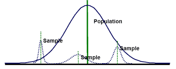
   We don’t get to pick a convenient group. Instead, random sampling allows us to have confidence that the sample represents the population. This process is a primary method for obtaining samples that mirrors the population on average. Random sampling produces statistics, such as the mean, that do not tend to be too high or too low. Using a random sample, we can generalize from the sample to the broader population.

统计代写|假设检验代写hypothesis testing代考|Population Parameters vs. Sample Statistics

A parameter is a value that describes a characteristic of an entire population, such as the population mean. Because you can rarely measure an entire population, you usually don’t know the real value of a parameter. In fact, parameter values are almost always unknowable. While we don’t know the value, it definitely exists.

For example, the average height of adult women in the United States is a parameter that has an exact value-we just don’t know what it is!
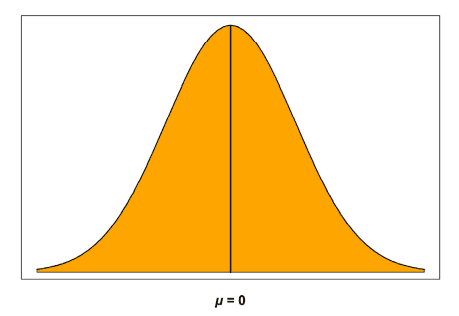
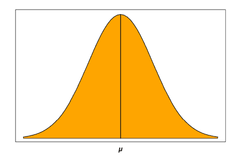
The population mean and standard deviation are two common parameters. In statistics, Greek symbols usually represent population parameters, such as $\mu(\mathrm{mu})$ for the mean and $\sigma$ (sigma) for the standard deviation.

A statistic is a characteristic of a sample. If you collect a sample and calculate the mean and standard deviation, these are sample statistics. Inferential statistics allow you to use sample statistics to make conclusions about a population. However, to draw valid conclusions, you must use representative sampling techniques. These techniques help ensure that samples produce unbiased estimates. Biased estimates are systematically too high or too low. You want unbiased estimates because they are correct on average. Use random sampling and other representative sampling methodologies to obtain unbiased estimates.
In inferential statistics, we use sample statistics to estimate population parameters. For example, if we collect a random sample of adult women in the United States and measure their heights, we can calculate the sample mean and use it as an unbiased estimate of the population mean. We can also create confidence intervals to obtain a range that the actual population value likely falls within.

假设检验代写

统计代写|假设检验代写hypothesis testing代考|Descriptive vs. Inferential Statistics

描述性统计汇总了您选择的组的数据。这个过程可以让你理解那组特定的观察结果。
描述性统计描述了一个样本。这很简单。您只需选取一个您感兴趣的组，记录有关组成员的数据，然后使用汇总统计数据和图表来展示组属性。使用描述性统计，没有不确定性，因为您只描述您实际测量的人或项目。例如，如果您测量两个班级的考试成绩，您就会知道两组的精确均值，并且可以毫无疑问地说明哪一个具有更高的均值。您不是要推断更多人口的属性。

然而，如果你想对人口进行推断，突然间你需要解决更多的问题。我们现在进入推论统计。对人群进行推论在科学中尤为重要，因为我们希望将结果应用于更大的人群，而不仅仅是研究中的特定样本。例如，如果我们正在测试一种新药，我们不想知道它只对小的、选定的实验组有效。我们想推断它将对更大的人群有效。我们希望将样本结果推广到样本之外的人。

推论统计从样本中获取数据，并对从中抽取样本的更大人群进行推断。因此，我们需要确信我们的样本准确地反映了人口。此要求会影响我们的流程。从广义上讲，我们必须做到以下几点：

1. 定义我们正在研究的人群。
2. 从该人群中抽取代表性样本。
3. 使用包含抽样误差的分析。
   我们不能选择一个方便的组。相反，随机抽样使我们有信心样本代表总体。此过程是获取反映总体平均情况的样本的主要方法。随机抽样产生的统计数据（例如均值）不会太高或太低。使用随机样本，我们可以从样本推广到更广泛的人群。

统计代写|假设检验代写hypothesis testing代考|Population Parameters vs. Sample Statistics

参数是描述整个总体特征的值，例如总体均值。因为您很少能测量整个总体，所以您通常不知道参数的真实值。事实上，参数值几乎总是不可知的。虽然我们不知道它的价值，但它确实存在。

例如，美国成年女性的平均身高是一个有确切数值的参数——我们只是不知道它是什么！
总体均值和标准差是两个常用参数。在统计学中，希腊符号通常代表人口参数，例如米(米在)对于均值和p(sigma) 为标准偏差。

统计量是样本的特征。如果您收集样本并计算平均值和标准偏差，这些就是样本统计数据。推论统计允许您使用样本统计来得出关于总体的结论。但是，要得出有效的结论，您必须使用代表性抽样技术。这些技术有助于确保样本产生无偏估计。有偏差的估计系统性地过高或过低。您需要无偏估计，因为它们平均是正确的。使用随机抽样和其他代表性抽样方法来获得无偏估计。
在推论统计中，我们使用样本统计来估计总体参数。例如，如果我们在美国随机收集成年女性样本并测量她们的身高，我们可以计算样本均值并将其用作总体均值的无偏估计。我们还可以创建置信区间以获得实际人口值可能落入的范围。

统计代写请认准statistics-lab™. statistics-lab™为您的留学生涯保驾护航。

随机过程代考

在概率论概念中，随机过程是随机变量的集合。 若一随机系统的样本点是随机函数，则称此函数为样本函数，这一随机系统全部样本函数的集合是一个随机过程。 实际应用中，样本函数的一般定义在时间域或者空间域。 随机过程的实例如股票和汇率的波动、语音信号、视频信号、体温的变化，随机运动如布朗运动、随机徘徊等等。

贝叶斯方法代考

贝叶斯统计概念及数据分析表示使用概率陈述回答有关未知参数的研究问题以及统计范式。后验分布包括关于参数的先验分布，和基于观测数据提供关于参数的信息似然模型。根据选择的先验分布和似然模型，后验分布可以解析或近似，例如，马尔科夫链蒙特卡罗 (MCMC) 方法之一。贝叶斯统计概念及数据分析使用后验分布来形成模型参数的各种摘要，包括点估计，如后验平均值、中位数、百分位数和称为可信区间的区间估计。此外，所有关于模型参数的统计检验都可以表示为基于估计后验分布的概率报表。

广义线性模型代考

广义线性模型（GLM）归属统计学领域，是一种应用灵活的线性回归模型。该模型允许因变量的偏差分布有除了正态分布之外的其它分布。

statistics-lab作为专业的留学生服务机构，多年来已为美国、英国、加拿大、澳洲等留学热门地的学生提供专业的学术服务，包括但不限于Essay代写，Assignment代写，Dissertation代写，Report代写，小组作业代写，Proposal代写，Paper代写，Presentation代写，计算机作业代写，论文修改和润色，网课代做，exam代考等等。写作范围涵盖高中，本科，研究生等海外留学全阶段，辐射金融，经济学，会计学，审计学，管理学等全球99%专业科目。写作团队既有专业英语母语作者，也有海外名校硕博留学生，每位写作老师都拥有过硬的语言能力，专业的学科背景和学术写作经验。我们承诺100%原创，100%专业，100%准时，100%满意。

机器学习代写

随着AI的大潮到来，Machine Learning逐渐成为一个新的学习热点。同时与传统CS相比，Machine Learning在其他领域也有着广泛的应用，因此这门学科成为不仅折磨CS专业同学的“小恶魔”，也是折磨生物、化学、统计等其他学科留学生的“大魔王”。学习Machine learning的一大绊脚石在于使用语言众多，跨学科范围广，所以学习起来尤其困难。但是不管你在学习Machine Learning时遇到任何难题，StudyGate专业导师团队都能为你轻松解决。

多元统计分析代考

基础数据: $N$ 个样本， $P$ 个变量数的单样本，组成的横列的数据表
变量定性: 分类和顺序；变量定量：数值
数学公式的角度分为: 因变量与自变量

时间序列分析代写

随机过程，是依赖于参数的一组随机变量的全体，参数通常是时间。 随机变量是随机现象的数量表现，其时间序列是一组按照时间发生先后顺序进行排列的数据点序列。通常一组时间序列的时间间隔为一恒定值（如1秒，5分钟，12小时，7天，1年），因此时间序列可以作为离散时间数据进行分析处理。研究时间序列数据的意义在于现实中，往往需要研究某个事物其随时间发展变化的规律。这就需要通过研究该事物过去发展的历史记录，以得到其自身发展的规律。

回归分析代写

多元回归分析渐进（Multiple Regression Analysis Asymptotics）属于计量经济学领域，主要是一种数学上的统计分析方法，可以分析复杂情况下各影响因素的数学关系，在自然科学、社会和经济学等多个领域内应用广泛。

MATLAB代写

MATLAB 是一种用于技术计算的高性能语言。它将计算、可视化和编程集成在一个易于使用的环境中，其中问题和解决方案以熟悉的数学符号表示。典型用途包括：数学和计算算法开发建模、仿真和原型制作数据分析、探索和可视化科学和工程图形应用程序开发，包括图形用户界面构建MATLAB 是一个交互式系统，其基本数据元素是一个不需要维度的数组。这使您可以解决许多技术计算问题，尤其是那些具有矩阵和向量公式的问题，而只需用 C 或 Fortran 等标量非交互式语言编写程序所需的时间的一小部分。MATLAB 名称代表矩阵实验室。MATLAB 最初的编写目的是提供对由 LINPACK 和 EISPACK 项目开发的矩阵软件的轻松访问，这两个项目共同代表了矩阵计算软件的最新技术。MATLAB 经过多年的发展，得到了许多用户的投入。在大学环境中，它是数学、工程和科学入门和高级课程的标准教学工具。在工业领域，MATLAB 是高效研究、开发和分析的首选工具。MATLAB 具有一系列称为工具箱的特定于应用程序的解决方案。对于大多数 MATLAB 用户来说非常重要，工具箱允许您学习和应用专业技术。工具箱是 MATLAB 函数（M 文件）的综合集合，可扩展 MATLAB 环境以解决特定类别的问题。可用工具箱的领域包括信号处理、控制系统、神经网络、模糊逻辑、小波、仿真等。

如果你也在 怎样代写假设检验hypothesis testing这个学科遇到相关的难题，请随时右上角联系我们的24/7代写客服。假设检验hypothesis testing是假设检验是统计学中的一种行为，分析者据此检验有关人口参数的假设。分析师采用的方法取决于所用数据的性质和分析的原因。假设检验是通过使用样本数据来评估假设的合理性。

statistics-lab™ 为您的留学生涯保驾护航 在假设检验hypothesis testing作业代写方面已经树立了自己的口碑, 保证靠谱, 高质且原创的统计Statistics代写服务。我们的专家在假设检验hypothesis testing代写方面经验极为丰富，各种假设检验hypothesis testing相关的作业也就用不着 说。

我们提供的假设检验hypothesis testing及其相关学科的代写，服务范围广, 其中包括但不限于:

• 时间序列分析Time-Series Analysis
• 马尔科夫过程 Markov process
• 随机最优控制stochastic optimal control
• 粒子滤波 Particle Filter
• 采样理论 sampling theory

统计代写|假设检验代写hypothesis testing代考|Some Measures of Location and Their Inuence Function

It is convenient to begin with quantiles. For any random variable $X$ with distribution $F$, the $q$ th quantile, say $x_q$, satisfies $F(x)=P\left(X \leq x_q\right)=q$, where $0<q<1$. For example, if $X$ is standard normal, the $0.8$ quantile is $x_{0.8}=0.84$ and $P(X \leq 0.84)=0.8$.

In the event that there are multiple $x$ values such that $F(x)=q$, the standard convention is to define the $q$ th quantile as the smallest value $x$ such that $F(x) \geq q$. For completeness, it is sometimes necessary to define the $q$ th quantile as $x_q=\inf {x: F(x) \geq q}$, where inf indicates infimum or greatest lower bound, but this is a detail that is not important here.

The $q$ th quantile has location and scale equivariance and it satisfies the other conditions for a measure of location given by Eqs (2.1) through (2.4), plus the Bickel-Lehmann condition. In so far as it is desired to have a measure of location that reflects the typical subject under study, the median, $x_{0.5}$, is a natural choice. The breakdown point of the median is $0.5$, and more generally the breakdown point of the $q$ th quantile is $1-q$ (e.g., Staudte and Sheather, 1990, p. 56).
For some distributions $x_q$ has qualitative robustness, but for others, including discrete distributions, it does not. In fact, even if $x_q$ has qualitative robustness at $F$, it is not qualitatively robust at $F_{x, \epsilon}$. That is, there are distributions that are arbitrarily close to $F$ for which $x_q$ is not qualitatively robust.

Letting $f(x)$ represent the probability density function, and assuming $f\left(x_q\right)>0$ and that $f\left(x_q\right)$ is continuous at $x_q$, the influence function of $x_q$ is
$$
I F_q(x)= \begin{cases}\frac{q-1}{f\left(x_q\right)}, & \text { if } xx_q .\end{cases}
$$
This influence function is bounded, so $x_q$ has infinitesimal robustness.

统计代写|假设检验代写hypothesis testing代考|The Winsorized Mean

One problem with the mean is that the tails of a distribution can dominate its value, and this is reflected by an unbounded influence function, a breakdown point of 0 , and a lack of qualitative robustness. Put in more practical terms, if a measure of location is intended to reflect what the typical subject is like, the mean can fail because its value can be inordinately influenced by a very small proportion of the subjects who fall in the tails of a distribution.
One strategy for dealing with this problem is to give less weight to values in the tails and pay more attention to those near the center. One specific strategy for implementing this idea is to Winsorize the distribution.
Let $F$ be any distribution, and let $x_\gamma$ and $x_{1-\gamma}$ be the $\gamma$ and $1-\gamma$ quantiles. Then a $\gamma$-Winsorized analog of $F$ is the distribution
$$
F_w(x)= \begin{cases}0, & \text { if } x<x_\gamma \ \gamma, & \text { if } x=x_\gamma \ F(x), & \text { if } x_\gamma<x<x_{1-\gamma} \ 1, & \text { if } x \geq x_{1-\gamma}\end{cases}
$$
In other words, the left tail is pulled in so that the probability of observing the value $x_\gamma$ is $\gamma$, and the probability of observing any value less than $x_\gamma$, after Winsorization, is 0 . Similarly, the right tail is pulled in so that, after Winsorization, the probability of observing a value greater than $x_{1-\gamma}$ is 0 . The mean of the Winsorized distribution is
$$
\mu_w=\int_{x_\gamma}^{x_{1-\gamma}} x d F(x)+\gamma\left(x_\gamma+x_{1-\gamma}\right) .
$$
In essence, the Winsorized mean pays more attention to the central portion of a distribution by transforming the tails. The result is that $\mu_w$ can be closer to the central portion of a distribution. It can be shown that $\mu_w$ satisfies Eqs (2.1) through (2.4), so it qualifies as a measure of location and it also satisfies the Bickel-Lehmann condition.

假设检验代写

统计代写|假设检验代写hypothesis testing代考|Some Measures of Location and Their Inuence Function

从分位数开始很方便。对于任意随机变量 $X$ 与分配 $F$ ，这 $q$ 第分位数，说 $x_q$ ，满足 $F(x)=P\left(X \leq x_q\right)=q$ ，在哪里 $00$ 然后 $f\left(x_q\right)$ 是连续的 $x_q$ ，的影响函数 $x_q$ 是
$$
I F_q(x)= \begin{cases}\frac{q-1}{f\left(x_q\right)}, & \text { if } x x_q .\end{cases}
$$
这个影响函数是有界的，所以 $x_q$ 具有无穷小的鲁棒性。

统计代写|假设检验代写hypothesis testing代考|The Winsorized Mean

均值的一个问题是分布的尾部可以支配其值，这反映在无界影响函数、故障点 0 和缺乏定性稳健性上。更实际 地说，如果位置度量旨在反映典型对象的情况，则平均值可能会失败，因为它的值可能会受到落在分布尾部的 一小部分对象的过度影响。
处理这个问题的一种策略是减少尾部的值的权重，更多地关注靠近中心的值。实现这个想法的一个具体策略是 Winsorize 分布。
让 $F$ 是任何分布，并让 $x_\gamma$ 和 $x_{1-\gamma}$ 成为 $\gamma$ 和 $1-\gamma$ 分位数。然后一个 $\gamma$-Winsorized模拟 $F$ 是分布
$F_w(x)=\left{0, \quad\right.$ if $x<x_\gamma \gamma, \quad$ if $x=x_\gamma F(x), \quad$ if $x_\gamma<x<x_{1-\gamma} 1, \quad$ if $x \geq x_{1-\gamma}$
换句话说，左边的尾巴被拉进来，使得观察值的概率 $x_\gamma$ 是 $\gamma$ ，以及观察到任何值小于的概率 $x_\gamma$ ，在 Winsorization 之后，是 0 。类似地，右尾被拉入，以便在 Winsorization 之后，观察到的值大于的概率 $x_{1-\gamma}$ 是 0 。Winsorized 分布的均值是
$$
\mu_w=\int_{x_\gamma}^{x_{1-\gamma}} x d F(x)+\gamma\left(x_\gamma+x_{1-\gamma}\right) .
$$
本质上，Winsorized 均值通过变换尾部更加关注分布的中心部分。结果是 $\mu_w$ 可以更接近分布的中心部分。可 以证明 $\mu_w$ 满足方程 (2.1) 到 (2.4)，因此它有资格作为位置的度量，并且它也满足 Bickel-Lehmann 条件。

统计代写请认准statistics-lab™. statistics-lab™为您的留学生涯保驾护航。

随机过程代考

在概率论概念中，随机过程是随机变量的集合。 若一随机系统的样本点是随机函数，则称此函数为样本函数，这一随机系统全部样本函数的集合是一个随机过程。 实际应用中，样本函数的一般定义在时间域或者空间域。 随机过程的实例如股票和汇率的波动、语音信号、视频信号、体温的变化，随机运动如布朗运动、随机徘徊等等。

贝叶斯方法代考

贝叶斯统计概念及数据分析表示使用概率陈述回答有关未知参数的研究问题以及统计范式。后验分布包括关于参数的先验分布，和基于观测数据提供关于参数的信息似然模型。根据选择的先验分布和似然模型，后验分布可以解析或近似，例如，马尔科夫链蒙特卡罗 (MCMC) 方法之一。贝叶斯统计概念及数据分析使用后验分布来形成模型参数的各种摘要，包括点估计，如后验平均值、中位数、百分位数和称为可信区间的区间估计。此外，所有关于模型参数的统计检验都可以表示为基于估计后验分布的概率报表。

广义线性模型代考

广义线性模型（GLM）归属统计学领域，是一种应用灵活的线性回归模型。该模型允许因变量的偏差分布有除了正态分布之外的其它分布。

statistics-lab作为专业的留学生服务机构，多年来已为美国、英国、加拿大、澳洲等留学热门地的学生提供专业的学术服务，包括但不限于Essay代写，Assignment代写，Dissertation代写，Report代写，小组作业代写，Proposal代写，Paper代写，Presentation代写，计算机作业代写，论文修改和润色，网课代做，exam代考等等。写作范围涵盖高中，本科，研究生等海外留学全阶段，辐射金融，经济学，会计学，审计学，管理学等全球99%专业科目。写作团队既有专业英语母语作者，也有海外名校硕博留学生，每位写作老师都拥有过硬的语言能力，专业的学科背景和学术写作经验。我们承诺100%原创，100%专业，100%准时，100%满意。

机器学习代写

随着AI的大潮到来，Machine Learning逐渐成为一个新的学习热点。同时与传统CS相比，Machine Learning在其他领域也有着广泛的应用，因此这门学科成为不仅折磨CS专业同学的“小恶魔”，也是折磨生物、化学、统计等其他学科留学生的“大魔王”。学习Machine learning的一大绊脚石在于使用语言众多，跨学科范围广，所以学习起来尤其困难。但是不管你在学习Machine Learning时遇到任何难题，StudyGate专业导师团队都能为你轻松解决。

多元统计分析代考

基础数据: $N$ 个样本， $P$ 个变量数的单样本，组成的横列的数据表
变量定性: 分类和顺序；变量定量：数值
数学公式的角度分为: 因变量与自变量

时间序列分析代写

随机过程，是依赖于参数的一组随机变量的全体，参数通常是时间。 随机变量是随机现象的数量表现，其时间序列是一组按照时间发生先后顺序进行排列的数据点序列。通常一组时间序列的时间间隔为一恒定值（如1秒，5分钟，12小时，7天，1年），因此时间序列可以作为离散时间数据进行分析处理。研究时间序列数据的意义在于现实中，往往需要研究某个事物其随时间发展变化的规律。这就需要通过研究该事物过去发展的历史记录，以得到其自身发展的规律。

回归分析代写

多元回归分析渐进（Multiple Regression Analysis Asymptotics）属于计量经济学领域，主要是一种数学上的统计分析方法，可以分析复杂情况下各影响因素的数学关系，在自然科学、社会和经济学等多个领域内应用广泛。

MATLAB代写

MATLAB 是一种用于技术计算的高性能语言。它将计算、可视化和编程集成在一个易于使用的环境中，其中问题和解决方案以熟悉的数学符号表示。典型用途包括：数学和计算算法开发建模、仿真和原型制作数据分析、探索和可视化科学和工程图形应用程序开发，包括图形用户界面构建MATLAB 是一个交互式系统，其基本数据元素是一个不需要维度的数组。这使您可以解决许多技术计算问题，尤其是那些具有矩阵和向量公式的问题，而只需用 C 或 Fortran 等标量非交互式语言编写程序所需的时间的一小部分。MATLAB 名称代表矩阵实验室。MATLAB 最初的编写目的是提供对由 LINPACK 和 EISPACK 项目开发的矩阵软件的轻松访问，这两个项目共同代表了矩阵计算软件的最新技术。MATLAB 经过多年的发展，得到了许多用户的投入。在大学环境中，它是数学、工程和科学入门和高级课程的标准教学工具。在工业领域，MATLAB 是高效研究、开发和分析的首选工具。MATLAB 具有一系列称为工具箱的特定于应用程序的解决方案。对于大多数 MATLAB 用户来说非常重要，工具箱允许您学习和应用专业技术。工具箱是 MATLAB 函数（M 文件）的综合集合，可扩展 MATLAB 环境以解决特定类别的问题。可用工具箱的领域包括信号处理、控制系统、神经网络、模糊逻辑、小波、仿真等。

如果你也在 怎样代写假设检验hypothesis testing这个学科遇到相关的难题，请随时右上角联系我们的24/7代写客服。假设检验hypothesis testing是假设检验是统计学中的一种行为，分析者据此检验有关人口参数的假设。分析师采用的方法取决于所用数据的性质和分析的原因。假设检验是通过使用样本数据来评估假设的合理性。

statistics-lab™ 为您的留学生涯保驾护航 在假设检验hypothesis testing作业代写方面已经树立了自己的口碑, 保证靠谱, 高质且原创的统计Statistics代写服务。我们的专家在假设检验hypothesis testing代写方面经验极为丰富，各种假设检验hypothesis testing相关的作业也就用不着 说。

我们提供的假设检验hypothesis testing及其相关学科的代写，服务范围广, 其中包括但不限于:

• 时间序列分析Time-Series Analysis
• 马尔科夫过程 Markov process
• 随机最优控制stochastic optimal control
• 粒子滤波 Particle Filter
• 采样理论 sampling theory

统计代写|假设检验代写hypothesis testing代考|Infinitesimal Robustness

To provide a relatively simple explanation of infinitesimal robustness, it helps to again consider the situation where $f(x)$ is any function, not necessarily a probability density function. Once more consider what restrictions might be imposed so that small changes in $x$ do not result in large changes in $f(x)$. One such condition is that it be differentiable and that the derivative be bounded. In symbols, if $f^{\prime}(x)$ is the derivative, it is required that $f^{\prime}(x)<B$ for some constant $B$. The function $f(x)=x^2$, for example, does not satisfy this condition because its derivative, $2 x$, increases without bound as $x$ gets large.
Analogs of derivatives of functionals exist and so a natural way of searching for robust measures of location is to focus on functionals that have a bounded derivative. In the statistics literature, the derivative of a functional, $T(F)$, is called the influence function of $T$ at $F$, which was introduced by Hampel (1968, 1974). Roughly, the influence function measures the relative extent a small perturbation in $F$ has on $T(F)$. Put another way, it reflects the (normed) limiting influence of adding one more observation, $x$, to a very large sample.
To provide a more precise description of the influence function, let $\Delta_x$ be a distribution where the value $x$ occurs with probability one. As is fairly evident, if $Y$ has distribution $\Delta_x$, then $P(Y \leq y)=0$ if $y<x$, and the mean of $Y$ is $E(Y)=x$.
Next, consider a mixture of two distributions where an observation is randomly sampled from distribution $F$ with probability $1-\epsilon$, otherwise sampling is from the distribution $\Delta_x$. That is, with probability $\epsilon$, the observed value is $x$. The resulting distribution is
$$
F_{x, c}=(1-\epsilon) F+\epsilon \Delta_x .
$$
It might help to notice the similarity between $F_{x, \epsilon}$ and the contaminated or mixed normal described in Chapter 1 . In the present situation, $F$ is any distribution, including normal distributions as a special case. Also notice the similarity with the influence curve in Chapter 1 .

统计代写|假设检验代写hypothesis testing代考|Quantitative Robustness

The third approach to judging some quantity that characterizes a distribution is the breakdown point, which addresses the notion of quantitative robustness. The general idea is to describe quantitatively the effect a small change in $F$ has on some functional $T(F)$.

Again consider $F_{x, \epsilon}=(1-\epsilon) F+\epsilon \Delta_x$, which has mean $(1-\epsilon) \mu+\epsilon x$. Thus, for any $\epsilon>0$, the mean goes to infinity as $x$ gets large. In particular, even when $\epsilon$ is arbitrarily close to 0 , in which case the Kolmogorov distance between $F_{x, \epsilon}$ and $F$ is small, the mean of $F_{x, \epsilon}$ can be made arbitrarily large by increasing $x$. The minimum value of $\epsilon$, for which a functional goes to infinity as $x$ gets large, is called the breakdown point. When necessary, the minimum value is replaced by the infimum or greatest lower bound. (This definition oversimplifies technical issues, but it suffices for present purposes. See Huber, 1981, Section $1.4$ for more details.) In the illustration, any $\epsilon>0$ causes the mean to go to infinity, so the breakdown point is 0 . In contrast, the median of a distribution has a breakdown point of $0.5$, and more generally the $\gamma$-trimmed mean, $\mu_t$, has a breakdown point of $\gamma$.
When searching for measures of dispersion, the breakdown point turns out to have considerable practical importance. In some cases the breakdown point is more important than the efficiency of any corresponding estimator. For the moment, it is merely noted that the standard deviation, $\sigma$, has a breakdown point of 0 , and this renders it unsatisfactory in various situations.

假设检验代写

统计代写|假设检验代写hypothesis testing代考|Infinitesimal Robustness

为了对无穷小稳健性提供一个相对简单的解释，再次考虑以下情况会有所帮助 $f(x)$ 是任何函数，不一定是概率 密度函数。再次考虑可能会施加哪些限制，以便在 $x$ 不会导致大的变化 $f(x)$. 一个这样的条件是它是可微的并且 导数是有界的。在符号中，如果 $f^{\prime}(x)$ 是导数，要求 $f^{\prime}(x)<B$ 对于一些常数 $B$. 功能 $f(x)=x^2$ ，例如，不满 足这个条件，因为它的导数， $2 x$ ，无限制地增加为 $x$ 变大。
泛函的导数存在类似物，因此寻找稳健的位置度量的自然方法是关注具有有界导数的泛函。在统计学文献中， 泛函的导数，T $T F)$ ，称为影响函数 $T$ 在 $F$ ，由 Hampel $(1968,1974)$ 引入。粗略地说，影响函数衡量的是一个小 样本。
为了更准确地描述影响函数，让 $\Delta_x$ 是一个分布，其中的价值 $x$ 以概率 1 发生。很明显，如果 $Y$ 有分布 $\Delta_x$ ，然 后 $P(Y \leq y)=0$ 如果 $y<x$, 以及的平均值 $Y$ 是 $E(Y)=x$.
接下来，考虑两种分布的混合，其中观察值是从分布中随机抽取的 $F$ 有概率 $1-\epsilon$ ，否则采样来自分布 $\Delta_x$. 也就 是说，以概率 $\epsilon$ ， 观测值为 $x$. 结果分布是
$$
F_{x, c}=(1-\epsilon) F+\epsilon \Delta_x .
$$
它可能有助于注意之间的相似性 $F_{x, \epsilon}$ 以及第 1 章中描述的污染或混合正态。在目前的情况下， $F$ 是任何分布， 包括作为特例的正态分布。还要注意与第 1 章中的影响曲线的相似性。

统计代写|假设检验代写hypothesis testing代考|Quantitative Robustness

判断某些表征分布的数量的第三种方法是击穿点，它解决了定量稳健性的概念。一般的想法是定量地描述一个 小变化的影响 $F$ 有一些功能 $T(F)$.
再考虑 $F_{x, \epsilon}=(1-\epsilon) F+\epsilon \Delta_x$ ，这意味着 $(1-\epsilon) \mu+\epsilon x$. 因此，对于任何 $\epsilon>0$ ，均值趋于无穷大 $x$ 变大。 特别地，即使当 $\epsilon$ 任意接近 0 ，在这种情况下，之间的 Kolmogorov 距离 $F_{x, \epsilon}$ 和 $F$ 很小，均值 $F_{x, \epsilon}$ 可以通过增加 任意大 $x$. 的最小值 $\epsilon$ ，其中一个泛函趋于无穷大 $x$ 变大，称为击穿点。必要时，最小值由下限或最大下限代替。 （此定义过于简化了技术问题，但足以满足当前的目的。参见 Huber，1981，第1.4了解更多详情。）在揷图 中，任何 $\epsilon>0$ 导致均值趋于无穷大，因此崩溃点为 0 。相比之下，分布的中位数有一个击穿点 $0.5$ ，更一般的 是 $\gamma$-修剪均值， $\mu_t$ ，有一个击穿点 $\gamma$.
在寻找色散测量时，击穿点具有相当大的实际重要性。在某些情况下，故障点比任何相应估算器的效率更重 要。目前，仅注意到标准偏差， $\sigma$ ，的击穿点为 0 ，这使得它在各种情况下都不能令人满意。

统计代写请认准statistics-lab™. statistics-lab™为您的留学生涯保驾护航。

随机过程代考

在概率论概念中，随机过程是随机变量的集合。 若一随机系统的样本点是随机函数，则称此函数为样本函数，这一随机系统全部样本函数的集合是一个随机过程。 实际应用中，样本函数的一般定义在时间域或者空间域。 随机过程的实例如股票和汇率的波动、语音信号、视频信号、体温的变化，随机运动如布朗运动、随机徘徊等等。

贝叶斯方法代考

贝叶斯统计概念及数据分析表示使用概率陈述回答有关未知参数的研究问题以及统计范式。后验分布包括关于参数的先验分布，和基于观测数据提供关于参数的信息似然模型。根据选择的先验分布和似然模型，后验分布可以解析或近似，例如，马尔科夫链蒙特卡罗 (MCMC) 方法之一。贝叶斯统计概念及数据分析使用后验分布来形成模型参数的各种摘要，包括点估计，如后验平均值、中位数、百分位数和称为可信区间的区间估计。此外，所有关于模型参数的统计检验都可以表示为基于估计后验分布的概率报表。

广义线性模型代考

广义线性模型（GLM）归属统计学领域，是一种应用灵活的线性回归模型。该模型允许因变量的偏差分布有除了正态分布之外的其它分布。

statistics-lab作为专业的留学生服务机构，多年来已为美国、英国、加拿大、澳洲等留学热门地的学生提供专业的学术服务，包括但不限于Essay代写，Assignment代写，Dissertation代写，Report代写，小组作业代写，Proposal代写，Paper代写，Presentation代写，计算机作业代写，论文修改和润色，网课代做，exam代考等等。写作范围涵盖高中，本科，研究生等海外留学全阶段，辐射金融，经济学，会计学，审计学，管理学等全球99%专业科目。写作团队既有专业英语母语作者，也有海外名校硕博留学生，每位写作老师都拥有过硬的语言能力，专业的学科背景和学术写作经验。我们承诺100%原创，100%专业，100%准时，100%满意。

机器学习代写

随着AI的大潮到来，Machine Learning逐渐成为一个新的学习热点。同时与传统CS相比，Machine Learning在其他领域也有着广泛的应用，因此这门学科成为不仅折磨CS专业同学的“小恶魔”，也是折磨生物、化学、统计等其他学科留学生的“大魔王”。学习Machine learning的一大绊脚石在于使用语言众多，跨学科范围广，所以学习起来尤其困难。但是不管你在学习Machine Learning时遇到任何难题，StudyGate专业导师团队都能为你轻松解决。

多元统计分析代考

基础数据: $N$ 个样本， $P$ 个变量数的单样本，组成的横列的数据表
变量定性: 分类和顺序；变量定量：数值
数学公式的角度分为: 因变量与自变量

时间序列分析代写

随机过程，是依赖于参数的一组随机变量的全体，参数通常是时间。 随机变量是随机现象的数量表现，其时间序列是一组按照时间发生先后顺序进行排列的数据点序列。通常一组时间序列的时间间隔为一恒定值（如1秒，5分钟，12小时，7天，1年），因此时间序列可以作为离散时间数据进行分析处理。研究时间序列数据的意义在于现实中，往往需要研究某个事物其随时间发展变化的规律。这就需要通过研究该事物过去发展的历史记录，以得到其自身发展的规律。

回归分析代写

多元回归分析渐进（Multiple Regression Analysis Asymptotics）属于计量经济学领域，主要是一种数学上的统计分析方法，可以分析复杂情况下各影响因素的数学关系，在自然科学、社会和经济学等多个领域内应用广泛。

MATLAB代写

MATLAB 是一种用于技术计算的高性能语言。它将计算、可视化和编程集成在一个易于使用的环境中，其中问题和解决方案以熟悉的数学符号表示。典型用途包括：数学和计算算法开发建模、仿真和原型制作数据分析、探索和可视化科学和工程图形应用程序开发，包括图形用户界面构建MATLAB 是一个交互式系统，其基本数据元素是一个不需要维度的数组。这使您可以解决许多技术计算问题，尤其是那些具有矩阵和向量公式的问题，而只需用 C 或 Fortran 等标量非交互式语言编写程序所需的时间的一小部分。MATLAB 名称代表矩阵实验室。MATLAB 最初的编写目的是提供对由 LINPACK 和 EISPACK 项目开发的矩阵软件的轻松访问，这两个项目共同代表了矩阵计算软件的最新技术。MATLAB 经过多年的发展，得到了许多用户的投入。在大学环境中，它是数学、工程和科学入门和高级课程的标准教学工具。在工业领域，MATLAB 是高效研究、开发和分析的首选工具。MATLAB 具有一系列称为工具箱的特定于应用程序的解决方案。对于大多数 MATLAB 用户来说非常重要，工具箱允许您学习和应用专业技术。工具箱是 MATLAB 函数（M 文件）的综合集合，可扩展 MATLAB 环境以解决特定类别的问题。可用工具箱的领域包括信号处理、控制系统、神经网络、模糊逻辑、小波、仿真等。

如果你也在 怎样代写假设检验hypothesis testing这个学科遇到相关的难题，请随时右上角联系我们的24/7代写客服。假设检验hypothesis testing是假设检验是统计学中的一种行为，分析者据此检验有关人口参数的假设。分析师采用的方法取决于所用数据的性质和分析的原因。假设检验是通过使用样本数据来评估假设的合理性。

statistics-lab™ 为您的留学生涯保驾护航 在假设检验hypothesis testing作业代写方面已经树立了自己的口碑, 保证靠谱, 高质且原创的统计Statistics代写服务。我们的专家在假设检验hypothesis testing代写方面经验极为丰富，各种假设检验hypothesis testing相关的作业也就用不着 说。

我们提供的假设检验hypothesis testing及其相关学科的代写，服务范围广, 其中包括但不限于:

• 时间序列分析Time-Series Analysis
• 马尔科夫过程 Markov process
• 随机最优控制stochastic optimal control
• 粒子滤波 Particle Filter
• 采样理论 sampling theory

统计代写|假设检验代写hypothesis testing代考|Basic Tools for Judging Robustness

There are three basic tools that are used to establish whether quantities such as measures of location and scale have good properties: qualitative robustness, quantitative robustness, and infinitesimal robustness. This section describes these tools in the context of location measures, but they are relevant to measures of scale as will become evident. These tools not only provide formal methods for judging a particular measure, they can be used to help derive measures that are robust.

Before continuing, it helps to be more formal about what is meant by a measure of location. A quantity that characterizes a distribution, such as the population mean, is said to be a measure of location if it satisfies four conditions, and a fifth is sometimes added. To describe them, let $X$ be a random variable with distribution $F$, and let $\theta(X)$ be some descriptive measure of $F$. Then $\theta(X)$ is said to be a measure of location if for any constants $a$ and $b$,
$$
\begin{gathered}
\theta(X+b)=\theta(X)+b \
\theta(-X)=-\theta(X) \
X \geq 0 \text { implies } \theta(X) \geq 0 \
\theta(a X)=a \theta(X) .
\end{gathered}
$$
The first condition is called location equivariance. It simply requires that if a constant $b$ is added to every possible value of $X$, a measure of location should be increased by the same amount. Let $E(X)$ denote the expected value of $X$. From basic principles, the population mean is location equivariant. That is, if $\theta(X)=E(X)=\mu$, then $\theta(X+b)=E(X+b)=\mu+b$. The first three conditions, taken together, imply that a measure of location should have a value within the range of possible values of $X$. The fourth condition is called scale equivariance. If the scale by which something is measured is altered by multiplying all possible values of $X$ by $a$, a measure of location should be altered by the same amount. In essence, results should be independent of the scale of measurement. As a simple example, if the typical height of a man is to be compared to the typical height of a woman, it should not matter whether the comparisons are made in inches or feet.

The fifth condition that is sometimes added was suggested by Bickel and Lehmann (1975). Let $F_x(x)=P(X \leq x)$ and $F_y(x)=P(Y \leq x)$ be the distributions corresponding to the random variables $X$ and $Y$. Then $X$ is said to be stochastically larger than $Y$ if for any $x$, $F_x(x) \leq F_y(x)$ with strict inequality for some $x$. If all the quantiles of $X$ are greater than the corresponding quantiles of $Y$, then $X$ is stochastically larger than $Y$. Bickel and Lehmann argue that if $X$ is stochastically larger than $Y$, then it should be the case that $\theta(X) \geq \theta(Y)$ if $\theta$ is to qualify as a measure of location. The population mean has this property.

统计代写|假设检验代写hypothesis testing代考|Qualitative Robustness

To understand qualitative robustness, it helps to begin by considering any function $f(x)$, not necessarily a probability density function. Suppose it is desired to impose a restriction on this function so that it does not change drastically with small changes in $x$. One way of doing this is to insist that $f(x)$ be continuous. If, for example, $f(x)=0$ for $x \leq 1$, but $f(x)=10,000$ for any $x>1$, the function is not continuous, and if $x=1$, an arbitrarily small increase in $x$ results in a large increase in $f(x)$.

A similar idea can be used when judging a measure of location. This is accomplished by viewing parameters as functionals. In the present context, a functional is just a rule that maps every distribution into a real number. For example, the population mean can be written as
$$
T(F)=E(X),
$$
where the expected value of $X$ depends on $F$. The role of $F$ becomes more explicit if expectation is written in integral form, in which case this last equation becomes
$$
T(F)=\int x d F(x) .
$$
If $X$ is discrete and the probability function corresponding to $F(x)$ is $f(x)$,
$$
T(F)=\sum x f(x),
$$
where the summation is over all possible values $x$ of $X$.
One advantage of viewing parameters as functionals is that the notion of continuity can be extended to them. Thus, if the goal is to have measures of location that are relatively unaffected by small shifts in $F$, a requirement that can be imposed is that when viewed as a functional, it is continuous. Parameters with this property are said to have qualitative robustness.
Let $\hat{F}$ be the usual empirical distribution. That is, for the random sample $X_1, \ldots, X_n, \hat{F}(x)$ is just the proportion of $X_i$ values less than or equal to $x$. An estimate of the functional $T(F)$ is obtained by replacing $F$ with $\hat{F}$. For example, when $T(F)=E(X)=\mu$, replacing $F$ with $\hat{F}$ yields the sample mean, $\bar{X}$. An important point is that qualitative robustness includes the idea that if $\hat{F}$ is close to $F$, in a sense to be made precise, then $T(\hat{F})$ should be close to $T(F)$. For example, if the empirical distribution represents a close approximation of $F$, then $\bar{X}$ should be a good approximation of $\mu$, but this is not always the case.

One more introductory remark should be made. From the technical point of view, continuity leads to the issue of how the difference between distributions should be measured. Here, the Kolmogorov distance is used. Other metrics play a role when addressing theoretical issues, but they go beyond the scope of this book. Readers interested in pursuing continuity, as it relates to robustness, can refer to Hampel (1968).

假设检验代写

统计代写|假设检验代写hypothesis testing代考|Basic Tools for Judging Robustness

可使用三种基本工具来确定位置和尺度等量度是否具有良好的属性：定性稳健性、定量稳健性和无穷小稳健 性。本节在位置测量的背景下描述这些工具，但它们与尺度测量相关，这一点将变得显而易见。这些工具不仅 提供了判断特定度量的正式方法，还可以用来帮助得出可靠的度量。
在继续之前，更正式地了解位置度量的含义会有所帮助。表征分布的量，如总体均值，如果满足四个条件，则 被称为位置度量，有时还会添加第五个条件。为了描述它们，让 $X$ 是一个具有分布的随机变量 $F$ ，然后让 $\theta(X)$ 是一些描述性措施 $F$. 然后 $\theta(X)$ 如果对于任何常数，则据说是位置的度量 $a$ 和 $b$ ，
$$
\theta(X+b)=\theta(X)+b \theta(-X)=-\theta(X) X \geq 0 \text { implies } \theta(X) \geq 0 \theta(a X)=a \theta(X) .
$$
第一个条件称为位置等方差。它只需要如果一个常量 $b$ 被添加到每个可能的值 $X$, 位置的度量应该增加相同的 量。让 $E(X)$ 表示期望值 $X$. 从基本原理来看，总体均值是位置等变的。也就是说，如果 $\theta(X)=E(X)=\mu$ ，然后 $\theta(X+b)=E(X+b)=\mu+b$. 前三个条件合在一起意味着位置度量的值应该在可能值的范围内 $X$ . 第四个条件称为尺度等方差。如果通过乘以所有可能的值来改变测量某物的尺度 $X$ 经过 $a$ ，个个位置的度量应该 改变相同的量。从本质上讲，结果应该独立于测量尺度。举一个简单的例子，如果要将男性的典型身高与女性 的典型身高进行比较，那么比较的单位是英寸还是英尺都无关紧要。
有时添加的第五个条件是由 Bickel 和 Lehmann (1975) 提出的。让 $F_x(x)=P(X \leq x)$ 和 $F_y(x)=P(Y \leq x)$ 是对应于随机变量的分布 $X$ 和 $Y$. 然后 $X$ 据说随机大于 $Y$ 如果有的话 $x, F_x(x) \leq F_y(x)$ 对某些人来说存在严格的不平等 $x$. 如果所有的分位数 $X$ 大于相应的分位数 $Y$ ，然后 $X$ 随机大于 $Y$. Bickel 和 Lehmann 认为，如果 $X$ 随机大于 $Y$ ，那么应该是这样的 $\theta(X) \geq \theta(Y)$ 如果 $\theta$ 有资格作为位置的衡量标准。总体 均值具有此属性。

统计代写|假设检验代写hypothesis testing代考|Qualitative Robustness

要理解定性稳健性，首先要考虑任何函数 $f(x)$ ，不一定是概率密度函数。假设希望对这个函数施加一个限制， 这样它就不会随看 $x$. 这样做的一种方法是坚持 $f(x)$ 是连续的。例如，如果 $f(x)=0$ 为了 $x \leq 1$ ，但 $f(x)=10,000$ 对于任何 $x>1$ ，函数不连续，如果 $x=1$ ，任意小的增加 $x$ 结果大大增加 $f(x)$.
在判断位置度量时可以使用类似的想法。这是通过将参数视为泛函来实现的。在当前上下文中，泛函只是将每 个分布映射到实数的规则。例如，总体均值可以写成
$$
T(F)=E(X),
$$
其中的期望值 $X$ 取决于 $F$. 的作用 $F$ 如果期望写成积分形式，则变得更加明确，在这种情况下，最后一个等式变 为
$$
T(F)=\int x d F(x) .
$$
如果 $X$ 是离散的，概率函数对应于 $F(x)$ 是 $f(x)$ ，
$$
T(F)=\sum x f(x),
$$
总和超过所有可能的值 $x$ 的 $X$.
将参数视为泛函的优点之一是连续性的概念可以扩展到它们。因此，如果目标是获得相对不受小变化影响的位 置度量 $F$ ，可以施加的一个要求是，当被视为泛函时，它是连续的。据说具有此属性的参数具有定性的鲁棒 性。
让 $\hat{F}$ 是通常的经验分布。也就是说，对于随机样本 $X_1, \ldots, X_n, \hat{F}(x)$ 只是比例 $X_i$ 值小于或等于 $x$. 函数的估 计 $T(F)$ 通过替换获得 $F$ 和 $\hat{F}$. 例如，当 $T(F)=E(X)=\mu$ ，替换 $F$ 和 $\hat{F}$ 产生样本均值， $\bar{X}$. 重要的一点是，
定性稳健性包括这样的想法: 如果 $\hat{F}$ 接近 $F$ ，在某种意义上要精确，那么 $T(\hat{F})$ 应该接近 $T(F)$. 例如，如果经 验分布表示一个近似值 $F$ ，然后 $\bar{X}$ 应该是一个很好的近似值 $\mu$ ，但情况并非总是如此。
还应作介绍性发言。从技术角度来看，连续性导致了如何衡量分布之间差异的问题。这里使用了 Kolmogorov 距离。其他指标在解决理论问题时发挥作用，但超出了本书的范围。有兴趣追求连续性的读者，因为它与鲁棒 性有关，可以参考 Hampel (1968)。

统计代写请认准statistics-lab™. statistics-lab™为您的留学生涯保驾护航。

随机过程代考

在概率论概念中，随机过程是随机变量的集合。 若一随机系统的样本点是随机函数，则称此函数为样本函数，这一随机系统全部样本函数的集合是一个随机过程。 实际应用中，样本函数的一般定义在时间域或者空间域。 随机过程的实例如股票和汇率的波动、语音信号、视频信号、体温的变化，随机运动如布朗运动、随机徘徊等等。

贝叶斯方法代考

贝叶斯统计概念及数据分析表示使用概率陈述回答有关未知参数的研究问题以及统计范式。后验分布包括关于参数的先验分布，和基于观测数据提供关于参数的信息似然模型。根据选择的先验分布和似然模型，后验分布可以解析或近似，例如，马尔科夫链蒙特卡罗 (MCMC) 方法之一。贝叶斯统计概念及数据分析使用后验分布来形成模型参数的各种摘要，包括点估计，如后验平均值、中位数、百分位数和称为可信区间的区间估计。此外，所有关于模型参数的统计检验都可以表示为基于估计后验分布的概率报表。

广义线性模型代考

广义线性模型（GLM）归属统计学领域，是一种应用灵活的线性回归模型。该模型允许因变量的偏差分布有除了正态分布之外的其它分布。

statistics-lab作为专业的留学生服务机构，多年来已为美国、英国、加拿大、澳洲等留学热门地的学生提供专业的学术服务，包括但不限于Essay代写，Assignment代写，Dissertation代写，Report代写，小组作业代写，Proposal代写，Paper代写，Presentation代写，计算机作业代写，论文修改和润色，网课代做，exam代考等等。写作范围涵盖高中，本科，研究生等海外留学全阶段，辐射金融，经济学，会计学，审计学，管理学等全球99%专业科目。写作团队既有专业英语母语作者，也有海外名校硕博留学生，每位写作老师都拥有过硬的语言能力，专业的学科背景和学术写作经验。我们承诺100%原创，100%专业，100%准时，100%满意。

机器学习代写

随着AI的大潮到来，Machine Learning逐渐成为一个新的学习热点。同时与传统CS相比，Machine Learning在其他领域也有着广泛的应用，因此这门学科成为不仅折磨CS专业同学的“小恶魔”，也是折磨生物、化学、统计等其他学科留学生的“大魔王”。学习Machine learning的一大绊脚石在于使用语言众多，跨学科范围广，所以学习起来尤其困难。但是不管你在学习Machine Learning时遇到任何难题，StudyGate专业导师团队都能为你轻松解决。

多元统计分析代考

基础数据: $N$ 个样本， $P$ 个变量数的单样本，组成的横列的数据表
变量定性: 分类和顺序；变量定量：数值
数学公式的角度分为: 因变量与自变量

时间序列分析代写

随机过程，是依赖于参数的一组随机变量的全体，参数通常是时间。 随机变量是随机现象的数量表现，其时间序列是一组按照时间发生先后顺序进行排列的数据点序列。通常一组时间序列的时间间隔为一恒定值（如1秒，5分钟，12小时，7天，1年），因此时间序列可以作为离散时间数据进行分析处理。研究时间序列数据的意义在于现实中，往往需要研究某个事物其随时间发展变化的规律。这就需要通过研究该事物过去发展的历史记录，以得到其自身发展的规律。

回归分析代写

多元回归分析渐进（Multiple Regression Analysis Asymptotics）属于计量经济学领域，主要是一种数学上的统计分析方法，可以分析复杂情况下各影响因素的数学关系，在自然科学、社会和经济学等多个领域内应用广泛。

MATLAB代写

MATLAB 是一种用于技术计算的高性能语言。它将计算、可视化和编程集成在一个易于使用的环境中，其中问题和解决方案以熟悉的数学符号表示。典型用途包括：数学和计算算法开发建模、仿真和原型制作数据分析、探索和可视化科学和工程图形应用程序开发，包括图形用户界面构建MATLAB 是一个交互式系统，其基本数据元素是一个不需要维度的数组。这使您可以解决许多技术计算问题，尤其是那些具有矩阵和向量公式的问题，而只需用 C 或 Fortran 等标量非交互式语言编写程序所需的时间的一小部分。MATLAB 名称代表矩阵实验室。MATLAB 最初的编写目的是提供对由 LINPACK 和 EISPACK 项目开发的矩阵软件的轻松访问，这两个项目共同代表了矩阵计算软件的最新技术。MATLAB 经过多年的发展，得到了许多用户的投入。在大学环境中，它是数学、工程和科学入门和高级课程的标准教学工具。在工业领域，MATLAB 是高效研究、开发和分析的首选工具。MATLAB 具有一系列称为工具箱的特定于应用程序的解决方案。对于大多数 MATLAB 用户来说非常重要，工具箱允许您学习和应用专业技术。工具箱是 MATLAB 函数（M 文件）的综合集合，可扩展 MATLAB 环境以解决特定类别的问题。可用工具箱的领域包括信号处理、控制系统、神经网络、模糊逻辑、小波、仿真等。

如果你也在 怎样代写假设检验hypothesis testing这个学科遇到相关的难题，请随时右上角联系我们的24/7代写客服。假设检验hypothesis testing是假设检验是统计学中的一种行为，分析者据此检验有关人口参数的假设。分析师采用的方法取决于所用数据的性质和分析的原因。假设检验是通过使用样本数据来评估假设的合理性。

statistics-lab™ 为您的留学生涯保驾护航 在假设检验hypothesis testing作业代写方面已经树立了自己的口碑, 保证靠谱, 高质且原创的统计Statistics代写服务。我们的专家在假设检验hypothesis testing代写方面经验极为丰富，各种假设检验hypothesis testing相关的作业也就用不着 说。

我们提供的假设检验hypothesis testing及其相关学科的代写，服务范围广, 其中包括但不限于:

• 时间序列分析Time-Series Analysis
• 马尔科夫过程 Markov process
• 随机最优控制stochastic optimal control
• 粒子滤波 Particle Filter
• 采样理论 sampling theory

统计代写|假设检验代写hypothesis testing代考|Finding the area under the normal curve

The area under the standard normal curve can be computed using the standard score. The Z score provides information on the position of a value compared to the average value using the distance to express the position by how many standard deviations the value falls above or below the average. The steps for finding the area under the standard normal curve require describing the standard normal table and then follow a few steps to extract the area from the table.

We use Table $\mathrm{A}$ in the Appendix to extract the area under the curve for $\mathrm{Z}$ values from 0 to 3 . The value of $\mathrm{Z}$ should be divided into two parts, the first part of the $\mathrm{Z}$ value in Table $\mathrm{A}$ is represented in the left-hand (first) column, the values of $\mathrm{Z}$ in the table start from 0 to 3 (nearest tenth), while the first (upper) row provides the second part of the $\mathrm{Z}$ value (second decimal place). We can use the same table to find the area under the curve for negative $Z$ values because of the symmetrical property of normal distribution.

Example 2.1: Compute the area to the left of a $\mathrm{Z}$ value: Compute the area under the standard normal curve to the left of a positive $\mathrm{Z}$ value of $2.13$.

Finding the area to the left of a positive $\mathrm{Z}$ value of $2.13$ requires using Table $\mathrm{A}$ in the Appendix for the standard normal. The value ” $2.13$ ” should be divided into two pieces, the first piece is ” $2.1$ ” and the second is ” $0.03$.” The exact area to the left of $2.13$ can be computed employing the steps below.

• The first step is to search for the position of “2.1” in the first vertical column of Table $2.1$ labeled $\mathrm{Z}$ to specify the first piece “2.1” of the number $2.13$ (highlighted row) [Table $2.1$ is a portion of the standard normal table in the Appendix (Table A)].
• The second step in finding the area is to move on the row of ” $2.1$ ” to the column labeled “0.03” (highlighted column), the point of intersection represents the requircd valuc which is $\mathbf{0 . 9 8 3 4}$ as shown in Table $2.1$ (bold value).
  The exact area to the left of $2.13$ is shown in Fig. $2.3$ (shaded area).

统计代写|假设检验代写hypothesis testing代考|Hypothesis testing for one sample mean

Consider a large sample of size $n(n \geq 30)$ that is selected from a normally distributed population and $Y$ represents a random variable of interest. A claim regarding the mean value of the variable of interest can be tested employing Z-test for one sample mean to make a decision regarding the mean value. The mathematical formula for computing the test statistic value for one sample Z-test is presented in Eq. (2.4).
$$
Z=\frac{\bar{Y}-\mu_0}{\sigma / \sqrt{n}}
$$
where,
$\bar{Y}$ represents the sample mean,
$\mu_0$ represents the claimed value (hypothesized mean),
$\sigma$ represents the population standard deviation, and
$n$ represents the sample size used.
The computed test statistic value obtained from the sample data (2.4) is usually used to make a decision to reject or not to reject the null hypothesis regarding the mean value of the variable of interest. The procedure of making a decision is to compare the test statistic value with the theoretical value (critical value) of the normal distribution or using a normal distribution curve.

Example 2.5: The concentration of cadmium of surface water: A professor at an environmental section wanted to verify the claim that the mean concentration of cadmium (Cd) of surface water in Juru River is $1.4(\mathrm{mg} / \mathrm{L})$. He selected 35 samples and tested for the cadmium concentration. The collected data showed that the mean concentration of cadmium is $1.6$ and the standard deviation of the population is $0.4$. A significance level of $\alpha=0.01$ is chosen to test the claim. Assume that the population is normally distributed.

The general procedure for conducting hypothesis testing can be used to make the decision regarding the mean concentration of cadmium of surface water in Juru River.
Step 1: Specify the null and alternative hypotheses
The mean concentration of cadmium of surface water in Juru River $(\mu)$ is $1.4$, this claim should be under the null hypothesis because the claim represents equality $(=)$. If the mean concentration of cadmium of surface water in Juru River is not equal to $1.4$, then two directions should be considered, the first direction could be the mean concentration of cadmium is greater than $1.4$ and the second direction could be the mean concentration of cadmium is less than 1.4. The two directions (greater than and less than) can be represented mathematically as $\neq$. Thus we can write the two hypotheses (null and alternative) as presented in Eq. (2.5).

假设检验代写

统计代写|假设检验代写hypothesis testing代考|Finding the area under the normal curve

标准正态曲线下的面积可以使用标准分数来计算。Z 分数提供了与平均值相比的值的位置信息，使用距离来表示位置，该位置通过值高于或低于平均值的多少标准偏差来表示。找到标准正态曲线下面积的步骤需要描述标准正态表，然后按照几个步骤从表中提取面积。

我们使用表一个在附录中提取曲线下的面积从值从 0 到 3 。的价值从应该分为两部分，第一部分从表中的值一个表示在左侧（第一）列中，的值从表中从 0 到 3（最近的十分之一）开始，而第一（上）行提供了第二部分从值（小数点后第二位）。我们可以使用同一张表来找到负曲线下的面积从值是因为正态分布的对称性。

例 2.1：计算 a 左边的面积从value：计算正态左侧标准正态曲线下的面积从的价值2.13.

找到正数左侧的区域从的价值2.13需要使用表一个在附录中为标准法线。价值 ”2.13“应该分成两块，第一块是”2.1“第二个是”0.03。” 左边的确切区域2.13可以使用以下步骤计算。

• 第一步是在Table的第一个垂直列中搜索“2.1”的位置2.1贴上标签从指定数字的第一个“2.1”2.13（突出显示的行）[表格2.1是附录（表 A）中标准正常表的一部分]。
• 找到该区域的第二步是移动“2.1”到标记为“0.03”的列（突出显示的列），交点表示所需的值，即0.9834如表所示2.1（粗体值）。
  左边的确切区域2.13如图所示。2.3（涂黑部分）。

统计代写|假设检验代写hypothesis testing代考|Hypothesis testing for one sample mean

考虑一个大样本 $n(n \geq 30)$ 是从一个正态分布的总体中选择的，并且 $Y$ 表示感兴趣的随机变量。可以对一个样 本均值使用 Z 检验来测试有关感兴趣变量平均值的声明，以做出关于平均值的决定。计算一个样本 Z 检验的检 验统计值的数学公式如公式 1 所示。(2.4)。
$$
Z=\frac{\bar{Y}-\mu_0}{\sigma / \sqrt{n}}
$$
在哪里，
$\bar{Y}$ 代表样本均值，
$\mu_0$ 表示声称的值（假设平均值），
$\sigma$ 表示总体标准差，并且
$n$ 表示使用的样本量。
从样本数据 (2.4) 获得的计算检验统计值通常用于决定拒绝或不拒绝关于感兴趣变量的平均值的原假设。做出决 定的过程是将检验统计值与正态分布的理论值 (临界值) 或使用正态分布曲线进行比较。
例 2.5：地表水中的镉浓度：环境科的一位教授想要验证以下说法，即汝鲁河地表水中镉 (Cd) 的平均浓度为 $1.4(\mathrm{mg} / \mathrm{L})$. 他选择了 35 个样品并测试了镉的浓度。收集的数据表明镉的平均浓度为 $1.6$ 并且总体的标准差是 $0.4$. 显着性水平 $\alpha=0.01$ 被选中来测试索赔。假设总体呈正态分布。
进行假设检验的一般程序可用于决定汝鲁河地表水中镉的平均浓度。
步骙 1：指定原假设和备择假设
Juru River 地表水中镉的平均浓度 $(\mu)$ 是 $1.4$ ，这个主张应该在零假设下，因为这个主张代表平等 $(=)$. 若汝鲁河 地表水镉平均浓度不等于 $1.4$ ，那么应该考虑两个方向，第一个方向可能是镉的平均浓度大于 $1.4$ 第二个方向可 能是镉的平均浓度小于 $1.4$ 。两个方向 (大于和小于) 可以在数学上表示为 $\neq$. 因此，我们可以写出方程式中提出 的两个假设（零假设和替代假设）。(2.5)。

统计代写请认准statistics-lab™. statistics-lab™为您的留学生涯保驾护航。

随机过程代考

在概率论概念中，随机过程是随机变量的集合。 若一随机系统的样本点是随机函数，则称此函数为样本函数，这一随机系统全部样本函数的集合是一个随机过程。 实际应用中，样本函数的一般定义在时间域或者空间域。 随机过程的实例如股票和汇率的波动、语音信号、视频信号、体温的变化，随机运动如布朗运动、随机徘徊等等。

贝叶斯方法代考

贝叶斯统计概念及数据分析表示使用概率陈述回答有关未知参数的研究问题以及统计范式。后验分布包括关于参数的先验分布，和基于观测数据提供关于参数的信息似然模型。根据选择的先验分布和似然模型，后验分布可以解析或近似，例如，马尔科夫链蒙特卡罗 (MCMC) 方法之一。贝叶斯统计概念及数据分析使用后验分布来形成模型参数的各种摘要，包括点估计，如后验平均值、中位数、百分位数和称为可信区间的区间估计。此外，所有关于模型参数的统计检验都可以表示为基于估计后验分布的概率报表。

广义线性模型代考

广义线性模型（GLM）归属统计学领域，是一种应用灵活的线性回归模型。该模型允许因变量的偏差分布有除了正态分布之外的其它分布。

statistics-lab作为专业的留学生服务机构，多年来已为美国、英国、加拿大、澳洲等留学热门地的学生提供专业的学术服务，包括但不限于Essay代写，Assignment代写，Dissertation代写，Report代写，小组作业代写，Proposal代写，Paper代写，Presentation代写，计算机作业代写，论文修改和润色，网课代做，exam代考等等。写作范围涵盖高中，本科，研究生等海外留学全阶段，辐射金融，经济学，会计学，审计学，管理学等全球99%专业科目。写作团队既有专业英语母语作者，也有海外名校硕博留学生，每位写作老师都拥有过硬的语言能力，专业的学科背景和学术写作经验。我们承诺100%原创，100%专业，100%准时，100%满意。

机器学习代写

随着AI的大潮到来，Machine Learning逐渐成为一个新的学习热点。同时与传统CS相比，Machine Learning在其他领域也有着广泛的应用，因此这门学科成为不仅折磨CS专业同学的“小恶魔”，也是折磨生物、化学、统计等其他学科留学生的“大魔王”。学习Machine learning的一大绊脚石在于使用语言众多，跨学科范围广，所以学习起来尤其困难。但是不管你在学习Machine Learning时遇到任何难题，StudyGate专业导师团队都能为你轻松解决。

多元统计分析代考

基础数据: $N$ 个样本， $P$ 个变量数的单样本，组成的横列的数据表
变量定性: 分类和顺序；变量定量：数值
数学公式的角度分为: 因变量与自变量

时间序列分析代写

随机过程，是依赖于参数的一组随机变量的全体，参数通常是时间。 随机变量是随机现象的数量表现，其时间序列是一组按照时间发生先后顺序进行排列的数据点序列。通常一组时间序列的时间间隔为一恒定值（如1秒，5分钟，12小时，7天，1年），因此时间序列可以作为离散时间数据进行分析处理。研究时间序列数据的意义在于现实中，往往需要研究某个事物其随时间发展变化的规律。这就需要通过研究该事物过去发展的历史记录，以得到其自身发展的规律。

回归分析代写

多元回归分析渐进（Multiple Regression Analysis Asymptotics）属于计量经济学领域，主要是一种数学上的统计分析方法，可以分析复杂情况下各影响因素的数学关系，在自然科学、社会和经济学等多个领域内应用广泛。

MATLAB代写

MATLAB 是一种用于技术计算的高性能语言。它将计算、可视化和编程集成在一个易于使用的环境中，其中问题和解决方案以熟悉的数学符号表示。典型用途包括：数学和计算算法开发建模、仿真和原型制作数据分析、探索和可视化科学和工程图形应用程序开发，包括图形用户界面构建MATLAB 是一个交互式系统，其基本数据元素是一个不需要维度的数组。这使您可以解决许多技术计算问题，尤其是那些具有矩阵和向量公式的问题，而只需用 C 或 Fortran 等标量非交互式语言编写程序所需的时间的一小部分。MATLAB 名称代表矩阵实验室。MATLAB 最初的编写目的是提供对由 LINPACK 和 EISPACK 项目开发的矩阵软件的轻松访问，这两个项目共同代表了矩阵计算软件的最新技术。MATLAB 经过多年的发展，得到了许多用户的投入。在大学环境中，它是数学、工程和科学入门和高级课程的标准教学工具。在工业领域，MATLAB 是高效研究、开发和分析的首选工具。MATLAB 具有一系列称为工具箱的特定于应用程序的解决方案。对于大多数 MATLAB 用户来说非常重要，工具箱允许您学习和应用专业技术。工具箱是 MATLAB 函数（M 文件）的综合集合，可扩展 MATLAB 环境以解决特定类别的问题。可用工具箱的领域包括信号处理、控制系统、神经网络、模糊逻辑、小波、仿真等。

如果你也在 怎样代写假设检验hypothesis testing这个学科遇到相关的难题，请随时右上角联系我们的24/7代写客服。假设检验hypothesis testing是假设检验是统计学中的一种行为，分析者据此检验有关人口参数的假设。分析师采用的方法取决于所用数据的性质和分析的原因。假设检验是通过使用样本数据来评估假设的合理性。

statistics-lab™ 为您的留学生涯保驾护航 在假设检验hypothesis testing作业代写方面已经树立了自己的口碑, 保证靠谱, 高质且原创的统计Statistics代写服务。我们的专家在假设检验hypothesis testing代写方面经验极为丰富，各种假设检验hypothesis testing相关的作业也就用不着 说。

我们提供的假设检验hypothesis testing及其相关学科的代写，服务范围广, 其中包括但不限于:

• 时间序列分析Time-Series Analysis
• 马尔科夫过程 Markov process
• 随机最优控制stochastic optimal control
• 粒子滤波 Particle Filter
• 采样理论 sampling theory

统计代写|假设检验代写hypothesis testing代考|Types of errors

Two types of errors are associated with hypothesis testing procedures in making a decision regarding the null hypothesis. A decision is usually made based on the sample information, and this decision could be correct or incorrect. The two types of errors are type I and type II errors.

The first type of error is called a type I error. This error occurs when we incorrectly decide to reject a true null hypothesis. A type I error is called the significance level $(\alpha)$

The second type of error is called a type II error. This error occurs when we fail to reject a false null hypothesis. The symbol for the probability of a type II error is $\beta$.
Note

• Type I and type II errors are inversely proportional; decreasing type I error $(\alpha)$ would increase type II error $\beta$, and increasing type I error $(\alpha)$ would decrease type II error $(\beta)$.
  Example 1.7: Specify type I and type II errors: Specify type I and type II errors for the claim which states that the mean concentration of cadmium (Cd) is $0.17 \mathrm{mg} / \mathrm{L}$.
  We need to identify the null and alternative hypotheses for this claim. The two hypotheses are given below:
  $$
  \begin{aligned}
  &H_0: \mu=0.17 \
  &H_1: \mu \neq 0.17
  \end{aligned}
  $$
  Type I error
  A type I error would occur when we incorrectly decide to reject a true null hypothesis. For the mean concentration of cadmium, a type I error would occur if the mean concentration of cadmium of surface water is $0.17 \mathrm{mg} / \mathrm{L}(\mu=0.17)$, but the information provided by the selected sample tells us to reject the claim that the mean concentration of cadmium of surface water is $0.17 \mathrm{mg} / \mathrm{L}$ and conclude that the mean concentration of cadmium of surface water is not equal to $0.17 \mathrm{mg} / \mathrm{L}$ $(\mu \neq 0.17)$
• A type II error would occur when we fail to reject a false null hypothesis. For the mean concentration of cadmium of surface water, a type II error would occur if the mean concentration of cadmium of surface water is not equal to $0.17 \mathrm{mg} / \mathrm{L}$ $(\mu \neq 0.17)$, but the information provided by the selected sample tells us not to reject the null hypothesis and conclude that the mean concentration of cadmium of surface water is equal to $0.17 \mathrm{mg} / \mathrm{L}(\mu=0.17)$.
• Correct decision
• A correct decision can be achieved in two cases: in the first case, if we do not reject the null hypothesis when it is true. The correct decision for this example is we do not reject the null hypothesis if the mean concentration of cadmium of surface water is equal to $0.17 \mathrm{mg} / \mathrm{L}(\mu=0.17)$.
• In the second case, if we reject the null hypothesis when it is false. The correct decision for this example is we reject the null hypothesis if the mean concentration of cadmium of surface water is not equal to $0.17 \mathrm{mg} / \mathrm{L}(\mu \neq 0.17)$.

统计代写|假设检验代写hypothesis testing代考|What is normal distribution

There are many distributions in statistics used to describe the behavior of different phenomena. One of the most important distributions is called normal distribution, or the bell curve due to its shape (bell-shaped). A Gaussian distribution is another name for normal distribution. The normal distribution curve is presented in Fig. 2.1.

Consider $Y$ represents a random variable that follows a normal distribution with mean $(\mu)$ and variance $\left(\sigma^2\right)$, then the normal probability distribution function is presented in Eq. (2.1).
$$
f(Y)=\frac{1}{\sqrt{2 \pi \sigma^2}} e^{-(Y-\mu)^2} / 2 \sigma^2 \quad-\infty<Y<\infty
$$
where,
$Y$ represents a random variable that is distributed normally $N\left(\mu, \sigma^2\right)$ or symbolized as $Y \sim N\left(\mu, \sigma^2\right)$,
$\pi=3.14$, and
$e \cong 2.71828$.

The properties of normal distribution curve are as follows:

1. The normal distribution curve is bell-shaped.
2. The shape of the normal distribution curve is symmetric about the mean.
3. The mean is at the center and divides the area into two equal parts.
4. The total area under the normal distribution curve is equal to 1 .
5. Most of the area under the curve falls between three standard deviations of the mean. The percentage of the area under one, two, and three standard deviations is given below.

• $68 \%$ of the points fall between one standard deviation of the mean;
• $95 \%$ of the points fall between two standard deviations of the mean;
• $99.7 \%$ of the points fall between three standard deviations of the mean.

假设检验代写

统计代写|假设检验代写hypothesis testing代考|Types of errors

在做出关于零假设的决定时，两种类型的错误与假设检验程序相关。通常根据样本信息做出决定，这个决定可能 是正确的，也可能是错误的。两种类型的错误是类型 | 和类型 || 错误。
第一种错误称为 I 型错误。当我们错误地决定拒绝一个真正的零假设时，就会发生此错误。第一类错误称为显着 性水平 $(\alpha)$
第二种错误称为 II 型错误。当我们末能拒绝错误的零假设时，就会发生此错误。II 类错误概率的符号是 $\beta$. 笔记

• I型和|l型错误成反比；减少第一类错误 $(\alpha)$ 会增加 II 型错误 $\beta$, 并增加 I 型错误 $(\alpha)$ 会减少第二类错误 $(\beta)$. 示例 1.7：指定 I 类和 II 类错误: 为声称镉 (Cd) 的平均浓度为 $0.17 \mathrm{mg} / \mathrm{L}$. 我们需要确定这一主张的零假设和替代假设。下面给出两个假设:
  $$
  H_0: \mu=0.17 \quad H_1: \mu \neq 0.17
  $$
  第一类
  错误 当我们错误地决定拒绝一个真实的零假设时，就会发生第一类错误。对于镉的平均浓度，如果地表水 镉的平均浓度为 $0.17 \mathrm{mg} / \mathrm{L}(\mu=0.17)$, 但所选样本提供的信息告诉我们拒绝声称地表水中镉的平均哝度 为 $0.17 \mathrm{mg} / \mathrm{L}$ 得出地表水中镉的平均浓度不等于 $0.17 \mathrm{mg} / \mathrm{L}(\mu \neq 0.17)$
• 当我们末能拒绝错误的零假设时，就佘发生 II 型错误。对于地表水镉的平均浓度，如果地表水镉的平均浓 度不等于 $0.17 \mathrm{mg} / \mathrm{L}(\mu \neq 0.17)$ ，但所选样本提供的信息告诉我们不要拒绝原假设并得出地表水镉的平均 浓度等于 $0.17 \mathrm{mg} / \mathrm{L}(\mu=0.17)$.
• 正确的决定
• 在两种情况下可以做出正确的决定: 在第一种情况下，如果我们在原假设为真时不拒绝它。此示例的正确 决策是，如果地表水中镉的平均浓度等于 $0.17 \mathrm{mg} / \mathrm{L}(\mu=0.17)$.
• 在第二种情况下，如果我们在原假设为假时拒绝原假设。此示例的正确决策是，如果地表水中镉的平均浓 度不等于 $0.17 \mathrm{mg} / \mathrm{L}(\mu \neq 0.17)$.

统计代写|假设检验代写hypothesis testing代考|What is normal distribution

统计中有许多分布用于描述不同现象的行为。最重要的分布之一称为正态分布，或由于其形状（钟形）而形成的 钟形曲线。高斯分布是正态分布的另一个名称。正态分布曲线如图 $2.1$ 所示。
考虑 $Y$ 表示服从均值正态分布的随机变量 $(\mu)$ 和方差 $\left(\sigma^2\right)$ ，则正态概率分布函数如方程式所示。(2.1)。
$$
f(Y)=\frac{1}{\sqrt{2 \pi \sigma^2}} e^{-(Y-\mu)^2} / 2 \sigma^2 \quad-\infty<Y<\infty
$$
在哪里，
$Y$ 表示一个正态分布的随机变量 $N\left(\mu, \sigma^2\right)$ 或符号为 $Y \sim N\left(\mu, \sigma^2\right)$,
$\pi=3.14$ ，和
$e \cong 2.71828$.
正态分布曲线的性质如下:

1. 正态分布曲线呈钟形。
2. 正态分布曲线的形状关于均值对称。
3. 平均值位于中心，将区域分成相等的两部分。
4. 正态分布曲线下的总面积等于 1 。
5. 曲线下的大部分区域落在平均值的三个标准差之间。下面给出了低于 1、2 和 3 个标准差的面积百分比。

• $68 \%$ 的点落在平均值的一个标准差之间；
• $95 \%$ 的点落在平均值的两个标准差之间;
• $99.7 \%$ 的点落在平均值的三个标准差之间。

统计代写请认准statistics-lab™. statistics-lab™为您的留学生涯保驾护航。

随机过程代考

在概率论概念中，随机过程是随机变量的集合。 若一随机系统的样本点是随机函数，则称此函数为样本函数，这一随机系统全部样本函数的集合是一个随机过程。 实际应用中，样本函数的一般定义在时间域或者空间域。 随机过程的实例如股票和汇率的波动、语音信号、视频信号、体温的变化，随机运动如布朗运动、随机徘徊等等。

贝叶斯方法代考

贝叶斯统计概念及数据分析表示使用概率陈述回答有关未知参数的研究问题以及统计范式。后验分布包括关于参数的先验分布，和基于观测数据提供关于参数的信息似然模型。根据选择的先验分布和似然模型，后验分布可以解析或近似，例如，马尔科夫链蒙特卡罗 (MCMC) 方法之一。贝叶斯统计概念及数据分析使用后验分布来形成模型参数的各种摘要，包括点估计，如后验平均值、中位数、百分位数和称为可信区间的区间估计。此外，所有关于模型参数的统计检验都可以表示为基于估计后验分布的概率报表。

广义线性模型代考

广义线性模型（GLM）归属统计学领域，是一种应用灵活的线性回归模型。该模型允许因变量的偏差分布有除了正态分布之外的其它分布。

statistics-lab作为专业的留学生服务机构，多年来已为美国、英国、加拿大、澳洲等留学热门地的学生提供专业的学术服务，包括但不限于Essay代写，Assignment代写，Dissertation代写，Report代写，小组作业代写，Proposal代写，Paper代写，Presentation代写，计算机作业代写，论文修改和润色，网课代做，exam代考等等。写作范围涵盖高中，本科，研究生等海外留学全阶段，辐射金融，经济学，会计学，审计学，管理学等全球99%专业科目。写作团队既有专业英语母语作者，也有海外名校硕博留学生，每位写作老师都拥有过硬的语言能力，专业的学科背景和学术写作经验。我们承诺100%原创，100%专业，100%准时，100%满意。

机器学习代写

随着AI的大潮到来，Machine Learning逐渐成为一个新的学习热点。同时与传统CS相比，Machine Learning在其他领域也有着广泛的应用，因此这门学科成为不仅折磨CS专业同学的“小恶魔”，也是折磨生物、化学、统计等其他学科留学生的“大魔王”。学习Machine learning的一大绊脚石在于使用语言众多，跨学科范围广，所以学习起来尤其困难。但是不管你在学习Machine Learning时遇到任何难题，StudyGate专业导师团队都能为你轻松解决。

多元统计分析代考

基础数据: $N$ 个样本， $P$ 个变量数的单样本，组成的横列的数据表
变量定性: 分类和顺序；变量定量：数值
数学公式的角度分为: 因变量与自变量

时间序列分析代写

随机过程，是依赖于参数的一组随机变量的全体，参数通常是时间。 随机变量是随机现象的数量表现，其时间序列是一组按照时间发生先后顺序进行排列的数据点序列。通常一组时间序列的时间间隔为一恒定值（如1秒，5分钟，12小时，7天，1年），因此时间序列可以作为离散时间数据进行分析处理。研究时间序列数据的意义在于现实中，往往需要研究某个事物其随时间发展变化的规律。这就需要通过研究该事物过去发展的历史记录，以得到其自身发展的规律。

回归分析代写

多元回归分析渐进（Multiple Regression Analysis Asymptotics）属于计量经济学领域，主要是一种数学上的统计分析方法，可以分析复杂情况下各影响因素的数学关系，在自然科学、社会和经济学等多个领域内应用广泛。

MATLAB代写

MATLAB 是一种用于技术计算的高性能语言。它将计算、可视化和编程集成在一个易于使用的环境中，其中问题和解决方案以熟悉的数学符号表示。典型用途包括：数学和计算算法开发建模、仿真和原型制作数据分析、探索和可视化科学和工程图形应用程序开发，包括图形用户界面构建MATLAB 是一个交互式系统，其基本数据元素是一个不需要维度的数组。这使您可以解决许多技术计算问题，尤其是那些具有矩阵和向量公式的问题，而只需用 C 或 Fortran 等标量非交互式语言编写程序所需的时间的一小部分。MATLAB 名称代表矩阵实验室。MATLAB 最初的编写目的是提供对由 LINPACK 和 EISPACK 项目开发的矩阵软件的轻松访问，这两个项目共同代表了矩阵计算软件的最新技术。MATLAB 经过多年的发展，得到了许多用户的投入。在大学环境中，它是数学、工程和科学入门和高级课程的标准教学工具。在工业领域，MATLAB 是高效研究、开发和分析的首选工具。MATLAB 具有一系列称为工具箱的特定于应用程序的解决方案。对于大多数 MATLAB 用户来说非常重要，工具箱允许您学习和应用专业技术。工具箱是 MATLAB 函数（M 文件）的综合集合，可扩展 MATLAB 环境以解决特定类别的问题。可用工具箱的领域包括信号处理、控制系统、神经网络、模糊逻辑、小波、仿真等。

如果你也在 怎样代写假设检验hypothesis testing这个学科遇到相关的难题，请随时右上角联系我们的24/7代写客服。假设检验hypothesis testing是假设检验是统计学中的一种行为，分析者据此检验有关人口参数的假设。分析师采用的方法取决于所用数据的性质和分析的原因。假设检验是通过使用样本数据来评估假设的合理性。

statistics-lab™ 为您的留学生涯保驾护航 在假设检验hypothesis testing作业代写方面已经树立了自己的口碑, 保证靠谱, 高质且原创的统计Statistics代写服务。我们的专家在假设检验hypothesis testing代写方面经验极为丰富，各种假设检验hypothesis testing相关的作业也就用不着 说。

我们提供的假设检验hypothesis testing及其相关学科的代写，服务范围广, 其中包括但不限于:

• 时间序列分析Time-Series Analysis
• 马尔科夫过程 Markov process
• 随机最优控制stochastic optimal control
• 粒子滤波 Particle Filter
• 采样理论 sampling theory

统计代写|假设检验代写hypothesis testing代考|The general procedure for performing statistical hypothesis testing

The general procedure for conducting hypothesis testing can be summarized by the steps given below.
Step 1: Specify the null and alternative hypotheses.
Step 2: Select the significance level $(\alpha)$ for the study.
Step 3: Use the sample information to calculate the test statistic value.
Step 4: Identify the critical and noncritical regions for the study.
Step 5: Make a decision and interpret the results.
We will discuss the general procedure step-by-step supported by examples where necessary.
Step 1: Specify the null and alternative hypotheses
We have studied this step earlier on how to write and specify the null and alternative hypotheses.
Step 2: Select the significance level $(\alpha)$ for the study
The significance level, usually called alpha $(\alpha)$, is also called the level of significance. Consider that the null hypothesis is true $\left(H_0\right)$, then the probability of rejecting the null hypothesis $\left(H_0\right)$ is called the alpha or significance level. The value of alpha refers to the significance of the results, and we usually select the value of alpha $(\alpha)$ to be $0.05$ or $0.01$.
Step 3: Use the sample information to calculate the test statistic value
The sample information (data) is used to calculate a value called the test statistic. This value is calculated using a specific mathematical formula for each distribution. Researchers use the test statistic value to make a decision to reject the null hypothesis or not.
Step 4: Identify the critical and noncritical regions for the study
The critical and noncritical regions are also called rejection and nonrejection regions; we should deliver the concept of critical values, and critical and noncritical regions.

The range of values of the test statistic that would reject the null hypothesis is called the critical region or the rejection region for a hypothesis testing.

The range of values of the test statistic that would not reject the null hypothesis is called the noncritical region or the nonrejection region for a hypothesis testing.
The value that is calculated from a probability distribution related to the problem under study is called the critical value. This value is used in hypothesis testing to differentiate the critical region (where $H_0$ should be rejected) from the noncritical region. We can calculate critical values for each distribution based on the significance level.

统计代写|假设检验代写hypothesis testing代考|Procedures for performing hypothesis testing

There are three procedures for making a decision in statistical hypothesis testing, which are the critical value procedure, $P$-value procedure, and confidence interval procedure. We will present the critical value procedure in this chapter, while the $P$ value and confidence interval procedures will be given in Chapter 6, The observed significance level ( $P$-value) procedure, and Chapter 7 , Interval estimation for one population, respectively.

1. Critical value procedure
   The critical value procedure is used to guide researchers and help in making a decision in statistical hypothesis testing. This procedure is also known as a traditional procedure. We can use the critical value procedure to make a decision regarding the null hypothesis using the test statistic value and the critical value related to the distribution used for solving the problem. The decision is made by comparing the two values (test statistic value and critical value). If the absolute test statistic value is greater than the critical value, the null hypothesis is rejected; otherwise the null hypothesis is not rejected. Or using the probability distribution curve, if the test statistic value falls in the critical region, the null hypothesis is rejected; otherwise the null hypothesis is not rejected.
2. We will employ the critical value procedure for making a decision regarding the onesample test for the mean value, proportion value, and variance value, while the other two procedures, the $P$-value and confidence interval procedures, will be given in Chapter 6 , The observed significance level ( $P$-value) procedure, and Chapter 7 , Interval estimation for one population, respectively, and then compare the results of various procedures.

假设检验代写

统计代写|假设检验代写hypothesis testing代考|The general procedure for performing statistical hypothesis testing

进行假设检验的一般程序可以通过下面给出的步骤进行总结。
第 1 步：指定原假设和备择假设。
步骤 2：选择显着性水平(一个)为研究。
第三步：利用样本信息计算检验统计量。
第 4 步：确定研究的关键和非关键区域。
第 5 步：做出决定并解释结果。
我们将在必要时通过示例逐步讨论一般程序。
第 1 步：指定零假设和备择假设
我们在前面已经研究过如何编写和指定零假设和备择假设。
步骤 2：选择显着性水平(一个)用于研究
的显着性水平，通常称为 alpha(一个)，也称为显着性水平。考虑原假设为真(H0), 那么拒绝原假设的概率(H0)称为阿尔法或显着性水平。alpha的值是指结果的显着性，我们通常选择alpha的值(一个)成为0.05或者0.01.
第三步：使用样本信息计算检验统计量
样本信息（数据）用于计算一个称为检验统计量的值。该值是使用每个分布的特定数学公式计算的。研究人员使用检验统计值来决定是否拒绝原假设。
步骤 4：确定研究
的关键和非关键区域 关键和非关键区域也称为拒绝和非拒绝区域；我们应该传递关键值以及关键和非关键区域的概念。

拒绝零假设的检验统计量值的范围称为假设检验的临界区或拒绝区。

不会拒绝原假设的检验统计量值的范围称为假设检验的非临界区域或非拒绝区域。
从与所研究问题相关的概率分布计算的值称为临界值。该值用于假设检验以区分临界区域（其中H0应该被拒绝）来自非关键区域。我们可以根据显着性水平计算每个分布的临界值。

统计代写|假设检验代写hypothesis testing代考|Procedures for performing hypothesis testing

在统计假设检验中做出决定有三个程序，即临界值程序，磷值过程和置信区间过程。我们将在本章中介绍临界值过程，而磷值和置信区间程序将在第 6 章中给出，观察到的显着性水平 (磷-value) 程序，以及第 7 章，一个总体的区间估计。

1. 临界值程序
   临界值程序用于指导研究人员并帮助在统计假设检验中做出决定。该程序也称为传统程序。我们可以使用临界值过程，使用检验统计值和与用于解决问题的分布相关的临界值来做出关于零假设的决定。通过比较两个值（检验统计值和临界值）来做出决定。如果绝对检验统计值大于临界值，则拒绝原假设；否则不拒绝原假设。或者利用概率分布曲线，如果检验统计量值落在临界区，则拒绝原假设；否则不拒绝原假设。
2. 我们将采用临界值程序来决定一个样本检验的平均值、比例值和方差值，而其他两个程序，即磷-值和置信区间程序，将在第 6 章中给出，观察显着性水平 (磷-value) 程序和第 7 章，一个总体的区间估计，然后比较各种程序的结果。

统计代写请认准statistics-lab™. statistics-lab™为您的留学生涯保驾护航。

随机过程代考

在概率论概念中，随机过程是随机变量的集合。 若一随机系统的样本点是随机函数，则称此函数为样本函数，这一随机系统全部样本函数的集合是一个随机过程。 实际应用中，样本函数的一般定义在时间域或者空间域。 随机过程的实例如股票和汇率的波动、语音信号、视频信号、体温的变化，随机运动如布朗运动、随机徘徊等等。

贝叶斯方法代考

贝叶斯统计概念及数据分析表示使用概率陈述回答有关未知参数的研究问题以及统计范式。后验分布包括关于参数的先验分布，和基于观测数据提供关于参数的信息似然模型。根据选择的先验分布和似然模型，后验分布可以解析或近似，例如，马尔科夫链蒙特卡罗 (MCMC) 方法之一。贝叶斯统计概念及数据分析使用后验分布来形成模型参数的各种摘要，包括点估计，如后验平均值、中位数、百分位数和称为可信区间的区间估计。此外，所有关于模型参数的统计检验都可以表示为基于估计后验分布的概率报表。

广义线性模型代考

广义线性模型（GLM）归属统计学领域，是一种应用灵活的线性回归模型。该模型允许因变量的偏差分布有除了正态分布之外的其它分布。

statistics-lab作为专业的留学生服务机构，多年来已为美国、英国、加拿大、澳洲等留学热门地的学生提供专业的学术服务，包括但不限于Essay代写，Assignment代写，Dissertation代写，Report代写，小组作业代写，Proposal代写，Paper代写，Presentation代写，计算机作业代写，论文修改和润色，网课代做，exam代考等等。写作范围涵盖高中，本科，研究生等海外留学全阶段，辐射金融，经济学，会计学，审计学，管理学等全球99%专业科目。写作团队既有专业英语母语作者，也有海外名校硕博留学生，每位写作老师都拥有过硬的语言能力，专业的学科背景和学术写作经验。我们承诺100%原创，100%专业，100%准时，100%满意。

机器学习代写

随着AI的大潮到来，Machine Learning逐渐成为一个新的学习热点。同时与传统CS相比，Machine Learning在其他领域也有着广泛的应用，因此这门学科成为不仅折磨CS专业同学的“小恶魔”，也是折磨生物、化学、统计等其他学科留学生的“大魔王”。学习Machine learning的一大绊脚石在于使用语言众多，跨学科范围广，所以学习起来尤其困难。但是不管你在学习Machine Learning时遇到任何难题，StudyGate专业导师团队都能为你轻松解决。

多元统计分析代考

基础数据: $N$ 个样本， $P$ 个变量数的单样本，组成的横列的数据表
变量定性: 分类和顺序；变量定量：数值
数学公式的角度分为: 因变量与自变量

时间序列分析代写

随机过程，是依赖于参数的一组随机变量的全体，参数通常是时间。 随机变量是随机现象的数量表现，其时间序列是一组按照时间发生先后顺序进行排列的数据点序列。通常一组时间序列的时间间隔为一恒定值（如1秒，5分钟，12小时，7天，1年），因此时间序列可以作为离散时间数据进行分析处理。研究时间序列数据的意义在于现实中，往往需要研究某个事物其随时间发展变化的规律。这就需要通过研究该事物过去发展的历史记录，以得到其自身发展的规律。

回归分析代写

多元回归分析渐进（Multiple Regression Analysis Asymptotics）属于计量经济学领域，主要是一种数学上的统计分析方法，可以分析复杂情况下各影响因素的数学关系，在自然科学、社会和经济学等多个领域内应用广泛。

MATLAB代写

MATLAB 是一种用于技术计算的高性能语言。它将计算、可视化和编程集成在一个易于使用的环境中，其中问题和解决方案以熟悉的数学符号表示。典型用途包括：数学和计算算法开发建模、仿真和原型制作数据分析、探索和可视化科学和工程图形应用程序开发，包括图形用户界面构建MATLAB 是一个交互式系统，其基本数据元素是一个不需要维度的数组。这使您可以解决许多技术计算问题，尤其是那些具有矩阵和向量公式的问题，而只需用 C 或 Fortran 等标量非交互式语言编写程序所需的时间的一小部分。MATLAB 名称代表矩阵实验室。MATLAB 最初的编写目的是提供对由 LINPACK 和 EISPACK 项目开发的矩阵软件的轻松访问，这两个项目共同代表了矩阵计算软件的最新技术。MATLAB 经过多年的发展，得到了许多用户的投入。在大学环境中，它是数学、工程和科学入门和高级课程的标准教学工具。在工业领域，MATLAB 是高效研究、开发和分析的首选工具。MATLAB 具有一系列称为工具箱的特定于应用程序的解决方案。对于大多数 MATLAB 用户来说非常重要，工具箱允许您学习和应用专业技术。工具箱是 MATLAB 函数（M 文件）的综合集合，可扩展 MATLAB 环境以解决特定类别的问题。可用工具箱的领域包括信号处理、控制系统、神经网络、模糊逻辑、小波、仿真等。

如果你也在 怎样代写假设检验hypothesis testing这个学科遇到相关的难题，请随时右上角联系我们的24/7代写客服。假设检验hypothesis testing是假设检验是统计学中的一种行为，分析者据此检验有关人口参数的假设。分析师采用的方法取决于所用数据的性质和分析的原因。假设检验是通过使用样本数据来评估假设的合理性。

statistics-lab™ 为您的留学生涯保驾护航 在假设检验hypothesis testing作业代写方面已经树立了自己的口碑, 保证靠谱, 高质且原创的统计Statistics代写服务。我们的专家在假设检验hypothesis testing代写方面经验极为丰富，各种假设检验hypothesis testing相关的作业也就用不着 说。

我们提供的假设检验hypothesis testing及其相关学科的代写，服务范围广, 其中包括但不限于:

• 时间序列分析Time-Series Analysis
• 马尔科夫过程 Markov process
• 随机最优控制stochastic optimal control
• 粒子滤波 Particle Filter
• 采样理论 sampling theory

统计代写|假设检验代写hypothesis testing代考|What is normal distribution

There are many distributions in statistics used to describe the behavior of different phenomena. One of the most important distributions is called normal distribution, or the bell curve due to its shape (bell-shaped). A Gaussian distribution is another name for normal distribution. The normal distribution curve is presented in Fig. 2.1.

Consider $Y$ represents a random variable that follows a normal distribution with mean $(\mu)$ and variance $\left(\sigma^2\right)$, then the normal probability distribution function is presented in Eq. (2.1).
$$
f(Y)=\frac{1}{\sqrt{2 \pi \sigma^2}} e^{-(Y-\mu)^2} / 2 \sigma^2 \quad-\infty<Y<\infty
$$
where,
$Y$ represents a random variable that is distributed normally $N\left(\mu, \sigma^2\right)$ or symbolized as
$$
\begin{aligned}
&Y \sim N\left(\mu, \sigma^2\right) \
&\pi=3.14, \text { and } \
&e \cong 2.71828
\end{aligned}
$$

The properties of normal distribution curve are as follows:

1. The normal distribution curve is bell-shaped.
2. The shape of the normal distribution curve is symmetric about the mean.
3. The mean is at the center and divides the area into two equal parts.
4. The total area under the normal distribution curve is equal to 1.
5. Most of the area under the curve falls between three standard deviations of the mean. The percentage of the area under one, two, and three standard deviations is given below.

• $68 \%$ of the points fall between one standard deviation of the mean;
• $95 \%$ of the points fall between two standard deviations of the mean;
• $99.7 \%$ of the points fall between three standard deviations of the mean.

统计代写|假设检验代写hypothesis testing代考|What is standard normal distribution

Consider that $Y$ represents a random variable that follows a normal distribution with mean (0) and variance (1), then the standard normal distribution function is presented in Eq. (2.2).
$$
f(Y)=\frac{1}{\sqrt{2 \pi}} e^{-Y^2 / 2}
$$
$Y$ represents a random variable that is distributed normally $N(0,1)$ or symbolized as $Y \sim N(0,1)$. The standard normal distribution has the same properties of normal distribution, the standard normal distribution curve is presented in Fig. 2.2.

We can convert any normal random variable to the standard normal distribution employing the formula given in Eq. (2.3).
$$
Z=\frac{Y-\mu}{\sigma}
$$
The formula in Eq. (2.3) is called the standard score.

假设检验代写

统计代写|假设检验代写假设检验代考|什么是正态分布

统计学中有许多分布用来描述不同现象的行为。最重要的分布之一被称为正态分布，或钟形曲线，因为它的形状(钟形)。高斯分布是正态分布的另一个名称。正态分布曲线如图2.1所示

假设$Y$代表一个服从正态分布的随机变量，其均值为$(\mu)$，方差为$\left(\sigma^2\right)$，则正态概率分布函数如式(2.1)所示。
$$
f(Y)=\frac{1}{\sqrt{2 \pi \sigma^2}} e^{-(Y-\mu)^2} / 2 \sigma^2 \quad-\infty<Y<\infty
$$
其中，
$Y$表示一个正态分布的随机变量$N\left(\mu, \sigma^2\right)$或表示为
$$
\begin{aligned}
&Y \sim N\left(\mu, \sigma^2\right) \
&\pi=3.14, \text { and } \
&e \cong 2.71828
\end{aligned}
$$

正态分布曲线的性质如下:

1. 正态分布曲线呈钟形。
2. 正态分布曲线的形状与均值是对称的。平均值位于中间，将该区域分成相等的两部分。
3. 正态分布曲线下面积之和为1。曲线下的大部分面积落在平均值的三个标准差之间。1、2和3个标准差以下的面积百分比如下:

$68 \%$的点落在均值的一个标准差之间， $95 \%$的点落在均值的两个标准差之间， $99.7 \%$的点落在均值的三个标准差之间，

统计代写|假设检验代写假设检验代考|什么是标准正态分布

假设$Y$代表一个服从均值(0)和方差(1)的正态分布的随机变量，则标准正态分布函数如式(2.2)所示。
$$
f(Y)=\frac{1}{\sqrt{2 \pi}} e^{-Y^2 / 2}
$$
$Y$表示正态分布的随机变量$N(0,1)$或符号为$Y \sim N(0,1)$。标准正态分布具有与正态分布相同的性质，标准正态分布曲线如图2.2所示

我们可以使用Eq.(2.3)中给出的公式将任何正态随机变量转换为标准正态分布。
$$
Z=\frac{Y-\mu}{\sigma}
$$
式(2.3)中的公式称为标准评分

统计代写请认准statistics-lab™. statistics-lab™为您的留学生涯保驾护航。

随机过程代考

在概率论概念中，随机过程是随机变量的集合。 若一随机系统的样本点是随机函数，则称此函数为样本函数，这一随机系统全部样本函数的集合是一个随机过程。 实际应用中，样本函数的一般定义在时间域或者空间域。 随机过程的实例如股票和汇率的波动、语音信号、视频信号、体温的变化，随机运动如布朗运动、随机徘徊等等。

贝叶斯方法代考

贝叶斯统计概念及数据分析表示使用概率陈述回答有关未知参数的研究问题以及统计范式。后验分布包括关于参数的先验分布，和基于观测数据提供关于参数的信息似然模型。根据选择的先验分布和似然模型，后验分布可以解析或近似，例如，马尔科夫链蒙特卡罗 (MCMC) 方法之一。贝叶斯统计概念及数据分析使用后验分布来形成模型参数的各种摘要，包括点估计，如后验平均值、中位数、百分位数和称为可信区间的区间估计。此外，所有关于模型参数的统计检验都可以表示为基于估计后验分布的概率报表。

广义线性模型代考

广义线性模型（GLM）归属统计学领域，是一种应用灵活的线性回归模型。该模型允许因变量的偏差分布有除了正态分布之外的其它分布。

statistics-lab作为专业的留学生服务机构，多年来已为美国、英国、加拿大、澳洲等留学热门地的学生提供专业的学术服务，包括但不限于Essay代写，Assignment代写，Dissertation代写，Report代写，小组作业代写，Proposal代写，Paper代写，Presentation代写，计算机作业代写，论文修改和润色，网课代做，exam代考等等。写作范围涵盖高中，本科，研究生等海外留学全阶段，辐射金融，经济学，会计学，审计学，管理学等全球99%专业科目。写作团队既有专业英语母语作者，也有海外名校硕博留学生，每位写作老师都拥有过硬的语言能力，专业的学科背景和学术写作经验。我们承诺100%原创，100%专业，100%准时，100%满意。

机器学习代写

随着AI的大潮到来，Machine Learning逐渐成为一个新的学习热点。同时与传统CS相比，Machine Learning在其他领域也有着广泛的应用，因此这门学科成为不仅折磨CS专业同学的“小恶魔”，也是折磨生物、化学、统计等其他学科留学生的“大魔王”。学习Machine learning的一大绊脚石在于使用语言众多，跨学科范围广，所以学习起来尤其困难。但是不管你在学习Machine Learning时遇到任何难题，StudyGate专业导师团队都能为你轻松解决。

多元统计分析代考

基础数据: $N$ 个样本， $P$ 个变量数的单样本，组成的横列的数据表
变量定性: 分类和顺序；变量定量：数值
数学公式的角度分为: 因变量与自变量

时间序列分析代写

随机过程，是依赖于参数的一组随机变量的全体，参数通常是时间。 随机变量是随机现象的数量表现，其时间序列是一组按照时间发生先后顺序进行排列的数据点序列。通常一组时间序列的时间间隔为一恒定值（如1秒，5分钟，12小时，7天，1年），因此时间序列可以作为离散时间数据进行分析处理。研究时间序列数据的意义在于现实中，往往需要研究某个事物其随时间发展变化的规律。这就需要通过研究该事物过去发展的历史记录，以得到其自身发展的规律。

回归分析代写

多元回归分析渐进（Multiple Regression Analysis Asymptotics）属于计量经济学领域，主要是一种数学上的统计分析方法，可以分析复杂情况下各影响因素的数学关系，在自然科学、社会和经济学等多个领域内应用广泛。

MATLAB代写

MATLAB 是一种用于技术计算的高性能语言。它将计算、可视化和编程集成在一个易于使用的环境中，其中问题和解决方案以熟悉的数学符号表示。典型用途包括：数学和计算算法开发建模、仿真和原型制作数据分析、探索和可视化科学和工程图形应用程序开发，包括图形用户界面构建MATLAB 是一个交互式系统，其基本数据元素是一个不需要维度的数组。这使您可以解决许多技术计算问题，尤其是那些具有矩阵和向量公式的问题，而只需用 C 或 Fortran 等标量非交互式语言编写程序所需的时间的一小部分。MATLAB 名称代表矩阵实验室。MATLAB 最初的编写目的是提供对由 LINPACK 和 EISPACK 项目开发的矩阵软件的轻松访问，这两个项目共同代表了矩阵计算软件的最新技术。MATLAB 经过多年的发展，得到了许多用户的投入。在大学环境中，它是数学、工程和科学入门和高级课程的标准教学工具。在工业领域，MATLAB 是高效研究、开发和分析的首选工具。MATLAB 具有一系列称为工具箱的特定于应用程序的解决方案。对于大多数 MATLAB 用户来说非常重要，工具箱允许您学习和应用专业技术。工具箱是 MATLAB 函数（M 文件）的综合集合，可扩展 MATLAB 环境以解决特定类别的问题。可用工具箱的领域包括信号处理、控制系统、神经网络、模糊逻辑、小波、仿真等。

如果你也在 怎样代写假设检验hypothesis testing这个学科遇到相关的难题，请随时右上角联系我们的24/7代写客服。假设检验hypothesis testing是假设检验是统计学中的一种行为，分析者据此检验有关人口参数的假设。分析师采用的方法取决于所用数据的性质和分析的原因。假设检验是通过使用样本数据来评估假设的合理性。

statistics-lab™ 为您的留学生涯保驾护航 在假设检验hypothesis testing作业代写方面已经树立了自己的口碑, 保证靠谱, 高质且原创的统计Statistics代写服务。我们的专家在假设检验hypothesis testing代写方面经验极为丰富，各种假设检验hypothesis testing相关的作业也就用不着 说。

我们提供的假设检验hypothesis testing及其相关学科的代写，服务范围广, 其中包括但不限于:

• 时间序列分析Time-Series Analysis
• 马尔科夫过程 Markov process
• 随机最优控制stochastic optimal control
• 粒子滤波 Particle Filter
• 采样理论 sampling theory

统计代写|假设检验代写hypothesis testing代考|Procedures for performing hypothesis testing

There are three procedures for making a decision in statistical hypothesis testing, which are the critical value procedure, $P$-value procedure, and confidence interval procedure. We will present the critical value procedure in this chapter, while the $P$ value and confidence interval procedures will be given in Chapter 6, The observed significance level ( $P$-value) procedure, and Chapter 7 , Interval estimation for one population, respectively.

1. Critical value procedure
   The critical value procedure is used to guide researchers and help in making a decision in statistical hypothesis testing. This procedure is also known as a traditional procedure. We can use the critical value procedure to make a decision regarding the null hypothesis using the test statistic value and the critical value related to the distribution used for solving the problem. The decision is made by comparing the two values (test statistic value and critical value). If the absolute test statistic value is greater than the critical value, the null hypothesis is rejected; otherwise the null hypothesis is not rejected. Or using the probability distribution curve, if the test statistic value falls in the critical region, the null hypothesis is rejected; otherwise the null hypothesis is not rejected.

We will employ the critical value procedure for making a decision regarding the onesample test for the mean value, proportion value, and variance value, while the other two procedures, the $P$-value and confidence interval procedures, will be given in Chapter 6 , The observed significance level ( $P$-value) procedure, and Chapter 7, Interval estimation for one population, respectively, and then compare the results of various procedures.

统计代写|假设检验代写hypothesis testing代考|Types of errors

Two types of errors are associated with hypothesis testing procedures in making a decision regarding the null hypothesis. A decision is usually made based on the sample information, and this decision could be correct or incorrect. The two types of errors are type I and type II errors.

The first type of error is called a type I error. This error occurs when we incorrectly decide to reject a true null hypothesis. A type I error is called the significance level $(\alpha)$

The second type of error is called a type II error. This error occurs when we fail to reject a false null hypothesis. The symbol for the probability of a type II error is $\beta$.
Note

• Type I and type II errors are inversely proportional; decreasing type I error $(\alpha)$ would increase type II error $\beta$, and increasing type I error $(\alpha)$ would decrease type II error $(\beta)$.
  Example 1.7: Specify type I and type II errors: Specify type I and type II errors for the claim which states that the mean concentration of cadmium $(\mathrm{Cd})$ is $0.17 \mathrm{mg} / \mathrm{L}$.
  We need to identify the null and alternative hypotheses for this claim. The two hypotheses are given below:
  $$
  \begin{aligned}
  &H_0: \mu=0.17 \
  &H_1: \mu \neq 0.17
  \end{aligned}
  $$
  Type I error
  A type I error would occur when we incorrectly decide to reject a true null hypothesis. For the mean concentration of cadmium, a type I error would occur if the mean concentration of cadmium of surface water is $0.17 \mathrm{mg} / \mathrm{L}(\mu=0.17)$, but the information provided by the selected sample tells us to reject the claim that the mean concentration of cadmium of surface water is $0.17 \mathrm{mg} / \mathrm{L}$ and conclude that the mean concentration of cadmium of surface water is not equal to $0.17 \mathrm{mg} / \mathrm{L}$ $(\mu \neq 0.17)$

A type II error would occur when we fail to reject a false null hypothesis. For the mean concentration of cadmium of surface water, a type II error would occur if the mean concentration of cadmium of surface water is not equal to $0.17 \mathrm{mg} / \mathrm{L}$ $(\mu \neq 0.17)$, but the information provided by the selected sample tells us not to reject the null hypothesis and conclude that the mean concentration of cadmium of surface water is equal to $0.17 \mathrm{mg} / \mathrm{L}(\mu=0.17)$.
Correct decision
A correct decision can be achieved in two cases: in the first case, if we do not reject the null hypothesis when it is true. The correct decision for this example is we do not reject the null hypothesis if the mean concentration of cadmium of surface water is equal to $0.17 \mathrm{mg} / \mathrm{L}(\mu=0.17)$.

In the second case, if we reject the null hypothesis when it is false. The correct decision for this example is we reject the null hypothesis if the mean concentration of cadmium of surface water is not equal to $0.17 \mathrm{mg} / \mathrm{L}(\mu \neq 0.17)$.

假设检验代写

统计代写|假设检验代写假设检验代考|执行假设检验的程序

. .

统计假设检验中有三种决策程序，分别是临界值程序、$P$ -值程序和置信区间程序。我们将在本章介绍临界值过程，而$P$值和置信区间过程将分别在第6章“观察显著性水平($P$ -value)”过程和第7章“一个总体的区间估计”中给出

1. 临界值程序
   临界值程序用于指导研究人员在统计假设检验中做出决策。这个程序也被称为传统程序。我们可以使用临界值程序，使用检验统计值和用于解决问题的分布相关的临界值，对零假设做出决策。通过比较两个值(检验统计值和临界值)来做出决策。如果绝对检验统计值大于临界值，则拒绝原假设;否则零假设不被拒绝。或者利用概率分布曲线，如果检验统计值落在临界区域，则拒绝原假设;

我们将使用临界值程序来对平均值、比例值和方差值的一个充分检验做出决定，而其他两个程序，$P$ -value和置信区间程序，将分别在第6章(观察显著性水平($P$ -value))程序和第7章(一个总体的区间估计)给出，然后比较各种程序的结果

统计代写|假设检验代写hypothesis testing代考|错误类型

两种类型的错误与关于零假设的决策的假设检验程序有关。决策通常是根据样本信息做出的，这个决策可能是正确的，也可能是错误的。这两种类型的错误是I型和II型错误

第一类错误被称为I型错误。当我们错误地决定拒绝一个真零假设时，就会出现这种错误。第一类错误称为显著性水平$(\alpha)$

第二类错误被称为第二类错误。当我们无法拒绝错误的零假设时，就会出现这种错误。第二类错误的概率符号为$\beta$。
注

• I型误差与II型误差成反比;递减型I型误差 $(\alpha)$ 会增加第二类误差吗 $\beta$， I型误差增加 $(\alpha)$ 会减少第二类误差吗 $(\beta)$
  例1.7:指定I型和II型错误:为声明镉的平均浓度的索赔指定I型和II型错误 $(\mathrm{Cd})$ 是 $0.17 \mathrm{mg} / \mathrm{L}$我们需要确定这一主张的零假设和备择假设。下面给出两个假设:
  $$
  \begin{aligned}
  &H_0: \mu=0.17 \
  &H_1: \mu \neq 0.17
  \end{aligned}
  $$当我们错误地决定拒绝一个真零假设时，就会发生I型错误。对于镉的平均浓度，如果地表水镉的平均浓度为，则会出现I型误差 $0.17 \mathrm{mg} / \mathrm{L}(\mu=0.17)$，但所选样品提供的信息告诉我们，我们不能接受地表水镉的平均浓度为 $0.17 \mathrm{mg} / \mathrm{L}$ 得出地表水中镉的平均浓度不等于 $0.17 \mathrm{mg} / \mathrm{L}$ $(\mu \neq 0.17)$

当我们不能拒绝错误的零假设时，就会发生第二类错误。对于地表水镉的平均浓度，如果地表水镉的平均浓度不等于$0.17 \mathrm{mg} / \mathrm{L}$$(\mu \neq 0.17)$，但所选样本提供的信息告诉我们不要拒绝原假设，而得出地表水镉的平均浓度等于$0.17 \mathrm{mg} / \mathrm{L}(\mu=0.17)$。
正确决策
正确决策可以在两种情况下实现:在第一种情况下，当零假设成立时，如果我们不拒绝它。对于这个例子，正确的决定是，如果地表水镉的平均浓度等于$0.17 \mathrm{mg} / \mathrm{L}(\mu=0.17)$，我们不拒绝零假设

在第二种情况下，如果我们在零假设为假时拒绝它。对于这个例子，正确的决定是，如果地表水镉的平均浓度不等于$0.17 \mathrm{mg} / \mathrm{L}(\mu \neq 0.17)$，我们拒绝零假设。

统计代写请认准statistics-lab™. statistics-lab™为您的留学生涯保驾护航。

随机过程代考

在概率论概念中，随机过程是随机变量的集合。 若一随机系统的样本点是随机函数，则称此函数为样本函数，这一随机系统全部样本函数的集合是一个随机过程。 实际应用中，样本函数的一般定义在时间域或者空间域。 随机过程的实例如股票和汇率的波动、语音信号、视频信号、体温的变化，随机运动如布朗运动、随机徘徊等等。

贝叶斯方法代考

贝叶斯统计概念及数据分析表示使用概率陈述回答有关未知参数的研究问题以及统计范式。后验分布包括关于参数的先验分布，和基于观测数据提供关于参数的信息似然模型。根据选择的先验分布和似然模型，后验分布可以解析或近似，例如，马尔科夫链蒙特卡罗 (MCMC) 方法之一。贝叶斯统计概念及数据分析使用后验分布来形成模型参数的各种摘要，包括点估计，如后验平均值、中位数、百分位数和称为可信区间的区间估计。此外，所有关于模型参数的统计检验都可以表示为基于估计后验分布的概率报表。

广义线性模型代考

广义线性模型（GLM）归属统计学领域，是一种应用灵活的线性回归模型。该模型允许因变量的偏差分布有除了正态分布之外的其它分布。

statistics-lab作为专业的留学生服务机构，多年来已为美国、英国、加拿大、澳洲等留学热门地的学生提供专业的学术服务，包括但不限于Essay代写，Assignment代写，Dissertation代写，Report代写，小组作业代写，Proposal代写，Paper代写，Presentation代写，计算机作业代写，论文修改和润色，网课代做，exam代考等等。写作范围涵盖高中，本科，研究生等海外留学全阶段，辐射金融，经济学，会计学，审计学，管理学等全球99%专业科目。写作团队既有专业英语母语作者，也有海外名校硕博留学生，每位写作老师都拥有过硬的语言能力，专业的学科背景和学术写作经验。我们承诺100%原创，100%专业，100%准时，100%满意。

机器学习代写

随着AI的大潮到来，Machine Learning逐渐成为一个新的学习热点。同时与传统CS相比，Machine Learning在其他领域也有着广泛的应用，因此这门学科成为不仅折磨CS专业同学的“小恶魔”，也是折磨生物、化学、统计等其他学科留学生的“大魔王”。学习Machine learning的一大绊脚石在于使用语言众多，跨学科范围广，所以学习起来尤其困难。但是不管你在学习Machine Learning时遇到任何难题，StudyGate专业导师团队都能为你轻松解决。

多元统计分析代考

基础数据: $N$ 个样本， $P$ 个变量数的单样本，组成的横列的数据表
变量定性: 分类和顺序；变量定量：数值
数学公式的角度分为: 因变量与自变量

时间序列分析代写

随机过程，是依赖于参数的一组随机变量的全体，参数通常是时间。 随机变量是随机现象的数量表现，其时间序列是一组按照时间发生先后顺序进行排列的数据点序列。通常一组时间序列的时间间隔为一恒定值（如1秒，5分钟，12小时，7天，1年），因此时间序列可以作为离散时间数据进行分析处理。研究时间序列数据的意义在于现实中，往往需要研究某个事物其随时间发展变化的规律。这就需要通过研究该事物过去发展的历史记录，以得到其自身发展的规律。

回归分析代写

多元回归分析渐进（Multiple Regression Analysis Asymptotics）属于计量经济学领域，主要是一种数学上的统计分析方法，可以分析复杂情况下各影响因素的数学关系，在自然科学、社会和经济学等多个领域内应用广泛。

MATLAB代写

MATLAB 是一种用于技术计算的高性能语言。它将计算、可视化和编程集成在一个易于使用的环境中，其中问题和解决方案以熟悉的数学符号表示。典型用途包括：数学和计算算法开发建模、仿真和原型制作数据分析、探索和可视化科学和工程图形应用程序开发，包括图形用户界面构建MATLAB 是一个交互式系统，其基本数据元素是一个不需要维度的数组。这使您可以解决许多技术计算问题，尤其是那些具有矩阵和向量公式的问题，而只需用 C 或 Fortran 等标量非交互式语言编写程序所需的时间的一小部分。MATLAB 名称代表矩阵实验室。MATLAB 最初的编写目的是提供对由 LINPACK 和 EISPACK 项目开发的矩阵软件的轻松访问，这两个项目共同代表了矩阵计算软件的最新技术。MATLAB 经过多年的发展，得到了许多用户的投入。在大学环境中，它是数学、工程和科学入门和高级课程的标准教学工具。在工业领域，MATLAB 是高效研究、开发和分析的首选工具。MATLAB 具有一系列称为工具箱的特定于应用程序的解决方案。对于大多数 MATLAB 用户来说非常重要，工具箱允许您学习和应用专业技术。工具箱是 MATLAB 函数（M 文件）的综合集合，可扩展 MATLAB 环境以解决特定类别的问题。可用工具箱的领域包括信号处理、控制系统、神经网络、模糊逻辑、小波、仿真等。

如果你也在 怎样代写假设检验hypothesis testing这个学科遇到相关的难题，请随时右上角联系我们的24/7代写客服。假设检验hypothesis testing是假设检验是统计学中的一种行为，分析者据此检验有关人口参数的假设。分析师采用的方法取决于所用数据的性质和分析的原因。假设检验是通过使用样本数据来评估假设的合理性。

statistics-lab™ 为您的留学生涯保驾护航 在假设检验hypothesis testing作业代写方面已经树立了自己的口碑, 保证靠谱, 高质且原创的统计Statistics代写服务。我们的专家在假设检验hypothesis testing代写方面经验极为丰富，各种假设检验hypothesis testing相关的作业也就用不着 说。

我们提供的假设检验hypothesis testing及其相关学科的代写，服务范围广, 其中包括但不限于:

• 时间序列分析Time-Series Analysis
• 马尔科夫过程 Markov process
• 随机最优控制stochastic optimal control
• 粒子滤波 Particle Filter
• 采样理论 sampling theory

统计代写|假设检验代写hypothesis testing代考|What is hypothesis testing

Hypothesis testing is a statistical technique used to make judgments regarding claims or statements related to populations. The opinion and definition of hypothesis testing with the general procedure of conducting the analysis are clarified before being applied to environmental data.

Any claim or statement made on population parameters (mean, standard deviation, and proportion) is called a hypothesis. A sample should be chosen from the population of interest to understand the behavior of the issue under investigation and make a judgment based on the collected sample information.

We can identify two types of hypotheses: the null hypothesis and the alternative hypothesis. The two hypotheses are mutually exclusive (they cannot occur together).

The null hypothesis is a statistical hypothesis that says no real difference exists between a population parameter (such as proportion, average, and standard deviation) and some claimed value (given value). The symbol for null hypothesis is $H_0$.

The alternative hypothesis is a statistical hypothesis that represents the opposite of the null hypothesis. An alternative hypothesis says that a real difference exists between a population parameter and a given value. The symbol for alternative hypothesis is $H_1$.

Three steps can be employed to specify the null and alternative hypotheses mathematically as given below.

1. Find out the hypothesis concerning the issue under investigation.
2. Translate the words of the null hypothesis into a mathematical expression.
3. Translate the words of the alternative hypothesis into a mathematical expression.
   Example 1.1: Specify the two hypotheses for the two-sided test: An environmentalist wishes to investigate a claim regarding the mean concentration of cadmium (Cd) of surface water. The environmentalist wants to examine the claim that the mean concentration of cadmium of surface water is $0.17 \mathrm{mg} / \mathrm{L}$.

The three steps for specifying the null and alternative hypotheses can be used to write the two hypotheses as shown below.

统计代写|假设检验代写hypothesis testing代考|The general procedure for performing statistical hypothesis testing

The general procedure for conducting hypothesis testing can be summarized by the steps given below.
Step 1: Specify the null and alternative hypotheses.
Step 2: Select the significance level $(\alpha)$ for the study.
Step 3: Use the sample information to calculate the test statistic value.
Step 4: Identify the critical and noncritical regions for the study.
Step 5: Make a decision and interpret the results.
We will discuss the general procedure step-by-step supported by examples where necessary.
Step 1: Specify the null and alternative hypotheses
We have studied this step earlier on how to write and specify the null and alternative hypotheses.
Step 2: Select the significance level $(\alpha)$ for the study
The significance level, usually called alpha $(\alpha)$, is also called the level of significance. Consider that the null hypothesis is true $\left(H_0\right)$, then the probability of rejecting the null hypothesis $\left(H_0\right)$ is called the alpha or significance level. The value of alpha refers to the significance of the results, and we usually select the value of alpha $(\alpha)$ to be $0.05$ or $0.01$.
Step 3: Use the sample information to calculate the test statistic value
The sample information (data) is used to calculate a value called the test statistic. This value is calculated using a specific mathematical formula for each distribution. Researchers use the test statistic value to make a decision to reject the null hypothesis or not.
Step 4: Identify the critical and noncritical regions for the study
The critical and noncritical regions are also called rejection and nonrejection regions; we should deliver the concept of critical values, and critical and noncritical regions.

The range of values of the test statistic that would reject the null hypothesis is called the critical region or the rejection region for a hypothesis testing.

The range of values of the test statistic that would not reject the null hypothesis is called the noncritical region or the nonrejection region for a hypothesis testing.
The value that is calculated from a probability distribution related to the problem under study is called the critical value. This value is used in hypothesis testing to differentiate the critical region (where $H_0$ should be rejected) from the noncritical region. We can calculate critical values for each distribution based on the significance level.

假设检验代写

统计代写|假设检验代写假设检验代考|什么是假设检验

假设检验是一种统计技术，用于对与总体相关的主张或陈述做出判断。在应用于环境数据之前，阐明了用进行分析的一般程序进行假设检验的观点和定义

任何关于总体参数(平均值、标准差和比例)的断言或陈述都被称为假设。应该从感兴趣的人群中选择一个样本，以理解被调查问题的行为，并根据收集到的样本信息做出判断

我们可以确定两种假设:零假设和备择假设。这两个假设是相互排斥的(它们不可能同时发生)

零假设是一种统计假设，它表示总体参数(如比例、平均值和标准差)与某些声称值(给定值)之间不存在真正的差异。零假设的符号是$H_0$。

备择假设是一个与零假设相反的统计假设。另一种假设认为，总体参数和给定值之间存在真正的差异。备择假设的符号是$H_1$。

如下所示，可以用三个步骤从数学上指定零假设和备择假设

找出关于正在调查的问题的假设。将零假设的单词翻译成一个数学表达式。将备择假设的文字翻译成数学表达式。例1.1:为双边检验指定两个假设:一位环境学家希望调查一项关于地表水镉(Cd)平均浓度的主张。环境学家想要检验地表水中镉的平均浓度是$0.17 \mathrm{mg} / \mathrm{L}$的说法

如下所示，指定零假设和备择假设的三步可用于编写两个假设

统计代写|假设检验代写假设检验代考|执行统计假设检验的一般程序

进行假设检验的一般程序可由以下步骤总结。第1步:指定空假设和备择假设。步骤2:选择研究的显著性水平$(\alpha)$。
步骤3:使用样本信息计算测试统计值。
步骤4:确定研究的关键区域和非关键区域。第五步:做出决定并解释结果。我们将在必要时通过示例逐步讨论一般过程。第一步:指定零假设和备择假设
我们之前已经学习了这一步如何编写和指定零假设和备择假设。
步骤2:为研究选择显著性水平$(\alpha)$
显著性水平，通常称为alpha $(\alpha)$，也称为显著性水平。假设零假设为真$\left(H_0\right)$，则拒绝零假设$\left(H_0\right)$的概率称为α或显著性水平。alpha的值表示结果的显著性，我们通常选择alpha的值$(\alpha)$为$0.05$或$0.01$。
步骤3:使用样本信息计算测试统计值
样本信息(数据)用于计算一个称为测试统计值的值。这个值是用每个分布的特定数学公式计算出来的。研究人员使用检验统计值来决定是否拒绝零假设。步骤4:识别研究的临界区和非临界区
临界区和非临界区也称为排斥区和非排斥区;我们应该提供临界值、临界区域和非临界区域的概念

拒绝原假设的检验统计值的范围称为临界区域或假设检验的拒绝区域

对于假设检验，不拒绝原假设的检验统计量的值的范围称为非临界区域或非拒绝区域。从与所研究问题相关的概率分布中计算出的值称为临界值。这个值用于假设检验，以区分临界区域(其中$H_0$应该被拒绝)和非临界区域。我们可以根据显著性水平计算每个分布的临界值

统计代写请认准statistics-lab™. statistics-lab™为您的留学生涯保驾护航。

随机过程代考

在概率论概念中，随机过程是随机变量的集合。 若一随机系统的样本点是随机函数，则称此函数为样本函数，这一随机系统全部样本函数的集合是一个随机过程。 实际应用中，样本函数的一般定义在时间域或者空间域。 随机过程的实例如股票和汇率的波动、语音信号、视频信号、体温的变化，随机运动如布朗运动、随机徘徊等等。

贝叶斯方法代考

贝叶斯统计概念及数据分析表示使用概率陈述回答有关未知参数的研究问题以及统计范式。后验分布包括关于参数的先验分布，和基于观测数据提供关于参数的信息似然模型。根据选择的先验分布和似然模型，后验分布可以解析或近似，例如，马尔科夫链蒙特卡罗 (MCMC) 方法之一。贝叶斯统计概念及数据分析使用后验分布来形成模型参数的各种摘要，包括点估计，如后验平均值、中位数、百分位数和称为可信区间的区间估计。此外，所有关于模型参数的统计检验都可以表示为基于估计后验分布的概率报表。

广义线性模型代考

广义线性模型（GLM）归属统计学领域，是一种应用灵活的线性回归模型。该模型允许因变量的偏差分布有除了正态分布之外的其它分布。

statistics-lab作为专业的留学生服务机构，多年来已为美国、英国、加拿大、澳洲等留学热门地的学生提供专业的学术服务，包括但不限于Essay代写，Assignment代写，Dissertation代写，Report代写，小组作业代写，Proposal代写，Paper代写，Presentation代写，计算机作业代写，论文修改和润色，网课代做，exam代考等等。写作范围涵盖高中，本科，研究生等海外留学全阶段，辐射金融，经济学，会计学，审计学，管理学等全球99%专业科目。写作团队既有专业英语母语作者，也有海外名校硕博留学生，每位写作老师都拥有过硬的语言能力，专业的学科背景和学术写作经验。我们承诺100%原创，100%专业，100%准时，100%满意。

机器学习代写

随着AI的大潮到来，Machine Learning逐渐成为一个新的学习热点。同时与传统CS相比，Machine Learning在其他领域也有着广泛的应用，因此这门学科成为不仅折磨CS专业同学的“小恶魔”，也是折磨生物、化学、统计等其他学科留学生的“大魔王”。学习Machine learning的一大绊脚石在于使用语言众多，跨学科范围广，所以学习起来尤其困难。但是不管你在学习Machine Learning时遇到任何难题，StudyGate专业导师团队都能为你轻松解决。

多元统计分析代考

基础数据: $N$ 个样本， $P$ 个变量数的单样本，组成的横列的数据表
变量定性: 分类和顺序；变量定量：数值
数学公式的角度分为: 因变量与自变量

时间序列分析代写

随机过程，是依赖于参数的一组随机变量的全体，参数通常是时间。 随机变量是随机现象的数量表现，其时间序列是一组按照时间发生先后顺序进行排列的数据点序列。通常一组时间序列的时间间隔为一恒定值（如1秒，5分钟，12小时，7天，1年），因此时间序列可以作为离散时间数据进行分析处理。研究时间序列数据的意义在于现实中，往往需要研究某个事物其随时间发展变化的规律。这就需要通过研究该事物过去发展的历史记录，以得到其自身发展的规律。

回归分析代写

多元回归分析渐进（Multiple Regression Analysis Asymptotics）属于计量经济学领域，主要是一种数学上的统计分析方法，可以分析复杂情况下各影响因素的数学关系，在自然科学、社会和经济学等多个领域内应用广泛。

MATLAB代写

MATLAB 是一种用于技术计算的高性能语言。它将计算、可视化和编程集成在一个易于使用的环境中，其中问题和解决方案以熟悉的数学符号表示。典型用途包括：数学和计算算法开发建模、仿真和原型制作数据分析、探索和可视化科学和工程图形应用程序开发，包括图形用户界面构建MATLAB 是一个交互式系统，其基本数据元素是一个不需要维度的数组。这使您可以解决许多技术计算问题，尤其是那些具有矩阵和向量公式的问题，而只需用 C 或 Fortran 等标量非交互式语言编写程序所需的时间的一小部分。MATLAB 名称代表矩阵实验室。MATLAB 最初的编写目的是提供对由 LINPACK 和 EISPACK 项目开发的矩阵软件的轻松访问，这两个项目共同代表了矩阵计算软件的最新技术。MATLAB 经过多年的发展，得到了许多用户的投入。在大学环境中，它是数学、工程和科学入门和高级课程的标准教学工具。在工业领域，MATLAB 是高效研究、开发和分析的首选工具。MATLAB 具有一系列称为工具箱的特定于应用程序的解决方案。对于大多数 MATLAB 用户来说非常重要，工具箱允许您学习和应用专业技术。工具箱是 MATLAB 函数（M 文件）的综合集合，可扩展 MATLAB 环境以解决特定类别的问题。可用工具箱的领域包括信号处理、控制系统、神经网络、模糊逻辑、小波、仿真等。