如果你也在 怎样代写随机控制Stochastic Control这个学科遇到相关的难题，请随时右上角联系我们的24/7代写客服。

随机控制或随机最优控制是控制理论的一个子领域，它涉及到观察中或驱动系统演变的噪声中存在的不确定性。

随机控制或随机最优控制是控制理论的一个子领域，它涉及到观察中或驱动系统进化的噪声中存在的不确定性。系统设计者以贝叶斯概率驱动的方式假设，具有已知概率分布的随机噪声会影响状态变量的演变和观察。随机控制的目的是设计受控变量的时间路径，以最小的成本执行所需的控制任务，尽管存在这种噪声，但以某种方式定义。

statistics-lab™ 为您的留学生涯保驾护航 在代写随机控制Stochastic Control方面已经树立了自己的口碑, 保证靠谱, 高质且原创的统计Statistics代写服务。我们的专家在代写随机控制Stochastic Control代写方面经验极为丰富，各种代写随机控制Stochastic Control相关的作业也就用不着说。

我们提供的随机控制Stochastic Control及其相关学科的代写，服务范围广, 其中包括但不限于:

• Statistical Inference 统计推断
• Statistical Computing 统计计算
• Advanced Probability Theory 高等概率论
• Advanced Mathematical Statistics 高等数理统计学
• (Generalized) Linear Models 广义线性模型
• Statistical Machine Learning 统计机器学习
• Longitudinal Data Analysis 纵向数据分析
• Foundations of Data Science 数据科学基础

统计代写|随机控制代写Stochastic Control代考|Third Degree Sensor Filtering Problem

This section presents an example of designing the optimal filter for a linear state over third degree polynomial observations, reducing it to the optimal filtering problem for a second degree polynomial state with partially measured linear part and second degree polynomial multiplicative noise over linear observations, where a conditionally Gaussian state initial condition is additionally assumed.
Let the unmeasured scalar state $x(t)$ satisfy the trivial linear equation
$$
d x(t)=d t+d w_1(t), \quad x(0)=x_0
$$
and the observation process be given by the scalar third degree sensor equation
$$
d y(t)=\left(x^3(t)+x(t)\right) d t+d w_2(t)
$$
where $w_1(t)$ and $w_2(t)$ are standard Wiener processes independent of each other and of a Gaussian random variable $x_0$ serving as the initial condition in (10). The filtering problem is to find the optimal estimate for the linear state (10), using the third degree sensor observations $(11)$.
Let us reformulate the problem, introducing the stochastic process $z(t)=h(x, t)=x^3(t)+$ $x(t)$. Using the Ito formula (see (31)) for the stochastic differential of the cubic function $h(x, t)=x^3(t)+x(t)$, where $x(t)$ satisfies the equation (10), the following equation is obtained for $z(t)$
$$
d z(t)=\left(1+3 x(t)+3 x^2(t)\right) d t+\left(3 x^2(t)+1\right) d w_1(t), z(0)=z_0
$$
Here, $\frac{\partial h(x, t)}{\partial x}=3 x^2(t)+1, \frac{1}{2} \frac{\partial^2 h(x, t)}{\partial x^2}=3 x(t)$, and $\frac{\partial h(x, t)}{\partial t}=0$; therefore, $f(x, t)=1+3 x(t)+$ $3 x^2(t)$ and $g(x, t)=3 x^2(t)+1$. The initial condition $z_0 \in R$ is considered a conditionally Gaussian random vector with respect to observations (see the paragraph following (4) for details). This assumption is quite admissible in the filtering framework, since the real distributions of $x(t)$ and $z(t)$ are unknown. In terms of the process $z(t)$, the observation equation (11) takes the form
$$
d y(t)=z(t) d t+d w_2(t)
$$

统计代写|随机控制代写Stochastic Control代考|Random signal expansion

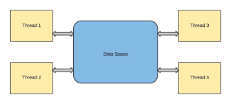
Let $\mathbf{S}$ be a zero mean, stationary, discrete-time random signal, made of $M$ successive samples and let $\left{s_1, s_2, \ldots, s_M\right}$ be a zero mean, uncorrelated random variable sequence, i.e.:
$$
E\left{s_n s_m\right}=E\left{s_m^2\right} \delta_{n, m}
$$
where $\delta_{n, m}$ denotes the Kronecker symbol.
It is possible to expand signal $\mathbf{S}$ into series of the form:
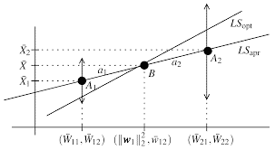
$$
\mathbf{S}=\sum_{m=1}^M s_m \boldsymbol{\Psi}{\mathbf{m}} $$ where $\left{\boldsymbol{\Psi}{\mathbf{m}}\right}_{m=1 \ldots M}$ corresponds to a $M$-dimensional deterministic basis. Vectors $\boldsymbol{\Psi}{\mathbf{m}}$ are linked to the choice of random variables sequence $\left{s_m\right}$, so there are many decompositions $(2)$ These vectors are determined by considering the mathematical expectation of the product of $s_m$ with the random signal $\mathbf{S}$. It comes: $$ \boldsymbol{\Psi}{\mathbf{m}}=\frac{1}{E\left{s_m^2\right}} E\left{s_m \mathbf{S}\right} .
$$
Classically and using a $M$-dimensional deterministic basis $\left{\boldsymbol{\Phi}{\mathrm{m}}\right}{m=1 \ldots M}$, the random variables $s_m$ can be expressed by the following relation:
$$
s_m=\mathbf{S}^T \boldsymbol{\Phi}{\mathbf{m}} $$ The determination of these random variables depends on the choice of the basis $\left{\boldsymbol{\Phi}{\mathrm{m}}\right}_{m=1 \ldots . M}$. We will use a basis, which provides the uncorrelation of the random variables. Using relations (1) and (4), we can show that the uncorrelation is ensured, when vectors $\boldsymbol{\Phi}{\mathrm{m}}$ are solution of the following quadratic form: $$ \boldsymbol{\Phi}{\mathbf{m}}{ }^T \boldsymbol{\Gamma}{\mathbf{S S}} \boldsymbol{\Phi}{\mathbf{n}}=E\left{s_m^2\right} \delta_{n, m},
$$
where $\Gamma_{\mathbf{S S}}$ represents the signal covariance.

随机控制代写

统计代写|随机控制代写Stochastic Control代考|Third Degree Sensor Filtering Problem

本节介绍了为三次多项式观测值的线性状态设计最优滤波器的示例，将其简化为具有部分测量的线性部分 和线性观测值的二次多项式乘法橾声的二次多项式状态的最优滤波问题，其中有条件地额外假设高斯状态 初始条件。
让末测量的标量状态 $x(t)$ 满足平凡的线性方程
$$
d x(t)=d t+d w_1(t), \quad x(0)=x_0
$$
并且观察过程由标量三次传感器方程给出
$$
d y(t)=\left(x^3(t)+x(t)\right) d t+d w_2(t)
$$
在哪里 $w_1(t)$ 和 $w_2(t)$ 是相互独立且独立于高斯随机变量的标准维纳过程 $x_0$ 作为 (10) 中的初始条件。 过滤问题是找到线性状态 (10) 的最优估计，使用三度传感器观察 $(11)$.
让我们重新表述问题，引入随机过程 $z(t)=h(x, t)=x^3(t)+x(t)$. 利用伊藤公式（见 (31) ) 求三 次函数的随机微分 $h(x, t)=x^3(t)+x(t)$ ，在哪里 $x(t)$ 满足式 $(10)$ ，则得到下式 $z(t)$
$$
d z(t)=\left(1+3 x(t)+3 x^2(t)\right) d t+\left(3 x^2(t)+1\right) d w_1(t), z(0)=z_0
$$
这里， $\frac{\partial h(x, t)}{\partial x}=3 x^2(t)+1, \frac{1}{2} \frac{\partial^2 h(x, t)}{\partial x^2}=3 x(t)$ ，和 $\frac{\partial h(x, t)}{\partial t}=0$; 所以， $f(x, t)=1+3 x(t)+$ $3 x^2(t)$ 和 $g(x, t)=3 x^2(t)+1$. 初始条件 $z_0 \in R$ 被认为是关于观测值的条件高斯随机向量 (有关详细 信息，请参见下面的 (4) 段) 。这个假设在过滤框架中是完全可以接受的，因为 $x(t)$ 和 $z(t)$ 是末知的。从 工艺上来说 $z(t)$ ，观察方程 (11) 的形式为
$$
d y(t)=z(t) d t+d w_2(t)
$$

统计代写|随机控制代写Stochastic Control代考|Random signal expansion

让 $\mathbf{S}$ 是一个零均值、平稳、离散时间的随机信号，由 $M$ 连续的样本，让 Meft{s_1,s_2, Vdots, s_Mıright} 是 一个零均值、不相关的随机变量序列，即:
EVleft{s_n s_m\right } } = E \backslash l e f t { s _ m ^ { \wedge } 2 \backslash r i g h t } \backslash d e l t a _ { n , m }
在哪里 $\delta_{n, m}$ 表示克罗内克符号。
可以扩展信号 $\mathbf{S}$ 成一系列的形式:
$$
\mathbf{S}=\sum_{m=1}^M s_m \mathbf{\Psi} \mathbf{m}
$$
机变量序列的选择有关 $\backslash$ 左 $\left{S _m \backslash\right.$ 右 $}$, 所以有很多分解(2)这些向量是通过考虑乘积的数学期望来确定的 $s_m$ 与随机信号S. 它来了: 用以下关系表示:
$$
s_m=\mathbf{S}^T \mathbf{\Phi} \mathbf{m}
$$
使用一个基础，它提供随机变量的不相关性。使用关系 (1) 和 (4)，我们可以证明当向量 $\boldsymbol{m} m$ 是以下二次 形式的解:
在哪里 $\Gamma_{\mathrm{SS}}$ 表示信号协方差。

统计代写请认准statistics-lab™. statistics-lab™为您的留学生涯保驾护航。

金融工程代写

金融工程是使用数学技术来解决金融问题。金融工程使用计算机科学、统计学、经济学和应用数学领域的工具和知识来解决当前的金融问题，以及设计新的和创新的金融产品。

非参数统计代写

非参数统计指的是一种统计方法，其中不假设数据来自于由少数参数决定的规定模型；这种模型的例子包括正态分布模型和线性回归模型。

广义线性模型代考

广义线性模型（GLM）归属统计学领域，是一种应用灵活的线性回归模型。该模型允许因变量的偏差分布有除了正态分布之外的其它分布。

术语 广义线性模型（GLM）通常是指给定连续和/或分类预测因素的连续响应变量的常规线性回归模型。它包括多元线性回归，以及方差分析和方差分析（仅含固定效应）。

有限元方法代写

有限元方法（FEM）是一种流行的方法，用于数值解决工程和数学建模中出现的微分方程。典型的问题领域包括结构分析、传热、流体流动、质量运输和电磁势等传统领域。

有限元是一种通用的数值方法，用于解决两个或三个空间变量的偏微分方程（即一些边界值问题）。为了解决一个问题，有限元将一个大系统细分为更小、更简单的部分，称为有限元。这是通过在空间维度上的特定空间离散化来实现的，它是通过构建对象的网格来实现的：用于求解的数值域，它有有限数量的点。边界值问题的有限元方法表述最终导致一个代数方程组。该方法在域上对未知函数进行逼近。[1] 然后将模拟这些有限元的简单方程组合成一个更大的方程系统，以模拟整个问题。然后，有限元通过变化微积分使相关的误差函数最小化来逼近一个解决方案。

tatistics-lab作为专业的留学生服务机构，多年来已为美国、英国、加拿大、澳洲等留学热门地的学生提供专业的学术服务，包括但不限于Essay代写，Assignment代写，Dissertation代写，Report代写，小组作业代写，Proposal代写，Paper代写，Presentation代写，计算机作业代写，论文修改和润色，网课代做，exam代考等等。写作范围涵盖高中，本科，研究生等海外留学全阶段，辐射金融，经济学，会计学，审计学，管理学等全球99%专业科目。写作团队既有专业英语母语作者，也有海外名校硕博留学生，每位写作老师都拥有过硬的语言能力，专业的学科背景和学术写作经验。我们承诺100%原创，100%专业，100%准时，100%满意。

随机分析代写

随机微积分是数学的一个分支，对随机过程进行操作。它允许为随机过程的积分定义一个关于随机过程的一致的积分理论。这个领域是由日本数学家伊藤清在第二次世界大战期间创建并开始的。

时间序列分析代写

随机过程，是依赖于参数的一组随机变量的全体，参数通常是时间。 随机变量是随机现象的数量表现，其时间序列是一组按照时间发生先后顺序进行排列的数据点序列。通常一组时间序列的时间间隔为一恒定值（如1秒，5分钟，12小时，7天，1年），因此时间序列可以作为离散时间数据进行分析处理。研究时间序列数据的意义在于现实中，往往需要研究某个事物其随时间发展变化的规律。这就需要通过研究该事物过去发展的历史记录，以得到其自身发展的规律。

回归分析代写

多元回归分析渐进（Multiple Regression Analysis Asymptotics）属于计量经济学领域，主要是一种数学上的统计分析方法，可以分析复杂情况下各影响因素的数学关系，在自然科学、社会和经济学等多个领域内应用广泛。

MATLAB代写

MATLAB 是一种用于技术计算的高性能语言。它将计算、可视化和编程集成在一个易于使用的环境中，其中问题和解决方案以熟悉的数学符号表示。典型用途包括：数学和计算算法开发建模、仿真和原型制作数据分析、探索和可视化科学和工程图形应用程序开发，包括图形用户界面构建MATLAB 是一个交互式系统，其基本数据元素是一个不需要维度的数组。这使您可以解决许多技术计算问题，尤其是那些具有矩阵和向量公式的问题，而只需用 C 或 Fortran 等标量非交互式语言编写程序所需的时间的一小部分。MATLAB 名称代表矩阵实验室。MATLAB 最初的编写目的是提供对由 LINPACK 和 EISPACK 项目开发的矩阵软件的轻松访问，这两个项目共同代表了矩阵计算软件的最新技术。MATLAB 经过多年的发展，得到了许多用户的投入。在大学环境中，它是数学、工程和科学入门和高级课程的标准教学工具。在工业领域，MATLAB 是高效研究、开发和分析的首选工具。MATLAB 具有一系列称为工具箱的特定于应用程序的解决方案。对于大多数 MATLAB 用户来说非常重要，工具箱允许您学习和应用专业技术。工具箱是 MATLAB 函数（M 文件）的综合集合，可扩展 MATLAB 环境以解决特定类别的问题。可用工具箱的领域包括信号处理、控制系统、神经网络、模糊逻辑、小波、仿真等。

R语言代写	问卷设计与分析代写
PYTHON代写	回归分析与线性模型代写
MATLAB代写	方差分析与试验设计代写
STATA代写	机器学习/统计学习代写
SPSS代写	计量经济学代写
EVIEWS代写	时间序列分析代写
EXCEL代写	深度学习代写
SQL代写	各种数据建模与可视化代写

如果你也在 怎样代写随机控制Stochastic Control这个学科遇到相关的难题，请随时右上角联系我们的24/7代写客服。

随机控制或随机最优控制是控制理论的一个子领域，它涉及到观察中或驱动系统演变的噪声中存在的不确定性。

随机控制或随机最优控制是控制理论的一个子领域，它涉及到观察中或驱动系统进化的噪声中存在的不确定性。系统设计者以贝叶斯概率驱动的方式假设，具有已知概率分布的随机噪声会影响状态变量的演变和观察。随机控制的目的是设计受控变量的时间路径，以最小的成本执行所需的控制任务，尽管存在这种噪声，但以某种方式定义。

statistics-lab™ 为您的留学生涯保驾护航 在代写随机控制Stochastic Control方面已经树立了自己的口碑, 保证靠谱, 高质且原创的统计Statistics代写服务。我们的专家在代写随机控制Stochastic Control代写方面经验极为丰富，各种代写随机控制Stochastic Control相关的作业也就用不着说。

我们提供的随机控制Stochastic Control及其相关学科的代写，服务范围广, 其中包括但不限于:

• Statistical Inference 统计推断
• Statistical Computing 统计计算
• Advanced Probability Theory 高等概率论
• Advanced Mathematical Statistics 高等数理统计学
• (Generalized) Linear Models 广义线性模型
• Statistical Machine Learning 统计机器学习
• Longitudinal Data Analysis 纵向数据分析
• Foundations of Data Science 数据科学基础

统计代写|随机控制代写Stochastic Control代考|Filtering Problem for Linear States over Polynomial Observations

Let $(\Omega, F, P)$ be a complete probability space with an increasing right-continuous family of $\sigma$-algebras $F_t, t \geq t_0$, and let $\left(W_1(t), F_t, t \geq t_0\right)$ and $\left(W_2(t), F_t, t \geq t_0\right)$ be independent Wiener processes. The $\bar{F}t$-measurable random process $(x(t), y(t)$ is described by a linear differential equation for the system state $$ d x(t)=\left(a_0(t)+a(t) x(t)\right) d t+b(t) d W_1(t), \quad x\left(t_0\right)=x_0 $$ and a nonlinear polynomial differential equation for the observation process $$ d y(t)=h(x, t) d t+B(t) d W_2(t) $$ Here, $x(t) \in R^n$ is the state vector and $y(t) \in R^m$ is the observation vector. The initial condition $x_0 \in R^n$ is a Gaussian vector such that $x_0, W_1(t)$, and $W_2(t)$ are independent. It is assumed that $B(t) B^T(t)$ is a positive definite matrix. All coefficients in (1)-(2) are deterministic functions of time of appropriate dimensions. The nonlinear function $h(x, t)$ forms the drift in the observation equation (2). The nonlinear function $h(x, t)$ is considered a polynomial of $n$ variables, components of the state vector $x(t) \in R^n$, with time-dependent coefficients. Since $x(t) \in R^n$ is a vector, this requires a special definition of the polynomial for $n>1$. In accordance with (27), a $p$-degree polynomial of a vector $x(t) \in R^n$ is regarded as a $p$-linear form of $n$ components of $x(t)$ $$ h(x, t)=\alpha_0(t)+\alpha_1(t) x+\alpha_2(t) x x^T+\ldots+\alpha_p(t) x \ldots p \text { times } \ldots x, $$ where $\alpha_0(t)$ is a vector of dimension $n, \alpha_1$ is a matrix of dimension $n \times n, \alpha_2$ is a $3 \mathrm{D}$ tensor of dimension $n \times n \times n, \alpha_p$ is an $(p+1) \mathrm{D}$ tensor of dimension $n \times \ldots(p+1)$ times $\ldots \times n$, and $x \times \ldots p$ times $\ldots \times x$ is a $p \mathrm{D}$ tensor of dimension $n \times \ldots p$ times $\ldots \times n$ obtained by $p$ times spatial multiplication of the vector $x(t)$ by itself (see (27) for more definition). Such a polynomial can also be expressed in the summation form $$ \begin{aligned} & h_k(x, t)=\alpha{0 k}(t)+\sum_i \alpha_{1 k i}(t) x_i(t)+\sum_{i j} \alpha_2 k i j(t) x_i(t) x_j(t)+\ldots \
& +\sum_{i_1 \ldots i_p} \alpha_{p k i_1 \ldots i_p}(t) x_{i_1}(t) \ldots x_{i_p}(t), \quad k, i, j, i_1, \ldots, i_p=1, \ldots, n .
\end{aligned}
$$
The estimation problem is to find the optimal estimate $\hat{x}(t)$ of the system state $x(t)$, based on the observation process $Y(t)={y(s), 0 \leq s \leq t}$, that minimizes the Euclidean 2-norm
$$
J=E\left[(x(t)-\hat{x}(t))^T(x(t)-\hat{x}(t)) \mid F_t^Y\right]
$$ at every time moment $t$. Here, $E\left[\xi(t) \mid F_t^Y\right]$ means the conditional expectation of a stochastic process $\xi(t)=(x(t)-\hat{x}(t))^T(x(t)-\hat{x}(t))$ with respect to the $\sigma$ – algebra $F_t^Y$ generated by the observation process $Y(t)$ in the interval $\left[t_0, t\right]$. As known (31), this optimal estimate is given by the conditional expectation
$$
\hat{x}(t)=m_x(t)=E\left(x(t) \mid F_t^Y\right)
$$
of the system state $x(t)$ with respect to the $\sigma$ – algebra $F_t^Y$ generated by the observation process $Y(t)$ in the interval $\left[t_0, t\right]$. As usual, the matrix function
$$
P(t)=E\left[\left(x(t)-m_x(t)\right)\left(x(t)-m_x(t)\right)^T \mid F_t^Y\right]
$$
is the estimation error variance.
The proposed solution to this optimal filtering problem is based on the formulas for the Ito differential of the optimal estimate and the estimation error variance (cited after (31)) and given in the following section.

统计代写|随机控制代写Stochastic Control代考|Optimal Filter for Linear States over Polynomial Observations

Let us reformulate the problem, introducing the stochastic process $z(t)=h(x, t)$. Using the Ito formula (see (31)) for the stochastic differential of the nonlinear function $h(x, t)$, where $x(t)$ satisfies the equation (1), the following equation is obtained for $z(t)$
$$
\begin{gathered}
d z(t)=\frac{\partial h(x, t)}{\partial x}\left(a_0(t)+a(t) x(t)\right) d t+\frac{\partial h(x, t)}{\partial t} d t+ \
\frac{1}{2} \frac{\partial^2 h(x, t)}{\partial x^2} b(t) b^T(t) d t+\frac{\partial h(x, t)}{\partial x} b(t) d W_1(t), \quad z(0)=z_0 .
\end{gathered}
$$
Note that the addition $\frac{1}{2} \frac{\partial^2 h(x, t)}{\partial x^2} b(t) b^T(t) d t$ appears in view of the second derivative in $x$ in the Ito formula.
The initial condition $z_0 \in R^n$ is considered a conditionally Gaussian random vector with respect to observations. This assumption is quite admissible in the filtering framework, since the real distributions of $x(t)$ and $z(t)$ are actually unknown. Indeed, as follows from (32), if only two lower conditional moments, expectation $m_0$ and variance $P_0$, of a random vector $\left[z_0, x_0\right]$ are available, the Gaussian distribution with the same parameters, $N\left(m_0, P_0\right)$, is the best approximation for the unknown conditional distribution of $\left[z_0, x_0\right]$ with respect to observations. This fact is also a corollary of the central limit theorem (33) in the probability theory.
A key point for further derivations is that the right-hand side of the equation (4) is a polynomial in $x$. Indeed, since $h(x, t)$ is a polynomial in $x$, the functions $\frac{\partial h(x, t)}{\partial x}, \frac{\partial h(x, t)}{\partial x} x(t), \frac{\partial h(x, t)}{\partial t}$, and $\frac{\partial^2 h(x, t)}{\partial x^2}$ are also polynomial in $x$. Thus, the equation (4) is a polynomial state equation with a polynomial multiplicative noise. It can be written in the compact form
$$
d z(t)=f(x, t) d t+g(x, t) d W_1(t), \quad z\left(t_0\right)=z_0,
$$
where
$$
\begin{gathered}
f(x, t)=\frac{\partial h(x, t)}{\partial x}\left(a_0(t)+a(t) x(t)\right)+\frac{\partial h(x, t)}{\partial t}+ \
\frac{1}{2} \frac{\partial^2 h(x, t)}{\partial x^2} b(t) b^T(t), \quad g(x, t)=\frac{\partial h(x, t)}{\partial x} b(t) .
\end{gathered}
$$

随机控制代写

统计代写|随机控制代写Stochastic Control代考|Filtering Problem for Linear States over Polynomial Observations

让 $(\Omega, F, P)$ 是一个完整的概率空间，具有递增的右连续族 $\sigma$-代数 $F_t, t \geq t_0$ ，然后让
$\left(W_1(t), F_t, t \geq t_0\right)$ 和 $\left(W_2(t), F_t, t \geq t_0\right)$ 是独立的维纳过程。这 $\bar{F} t$-可测随机过程 $(x(t), y(t)$ 由系统 状态的线性微分方程描述
$$
d x(t)=\left(a_0(t)+a(t) x(t)\right) d t+b(t) d W_1(t), \quad x\left(t_0\right)=x_0
$$
和观测过程的非线性多项式微分方程
$$
d y(t)=h(x, t) d t+B(t) d W_2(t)
$$
这里， $x(t) \in R^n$ 是状态向量和 $y(t) \in R^m$ 是观测向量。初始条件 $x_0 \in R^n$ 是一个高斯向量，使得 $x_0, W_1(t)$ ，和 $W_2(t)$ 是独立的。据推测 $B(t) B^T(t)$ 是正定矩阵。(1)-(2)中的所有系数都是适当维度的 时间的确定性函数。非线性函数 $h(x, t)$ 形成观测方程 (2) 中的漂移。非线性函数 $h(x, t)$ 被认为是多项 式 $n$ 变量，状态向量的分量 $x(t) \in R^n$ ，具有随时间变化的系数。自从 $x(t) \in R^n$ 是一个向量，这需要 一个特殊的多项式定义 $n>1$. 根据（27)，一个 向量的次多项式 $x(t) \in R^n$ 被视为 $p$-线性形式 $n$ 的组 成部分 $x(t)$
$$
h(x, t)=\alpha_0(t)+\alpha_1(t) x+\alpha_2(t) x x^T+\ldots+\alpha_p(t) x \ldots p \text { times } \ldots x,
$$
在哪里 $\alpha_0(t)$ 是维度向量 $n, \alpha_1$ 是维度矩阵 $n \times n, \alpha_2$ 是一个 $3 \mathrm{D}$ 维度张量 $n \times n \times n, \alpha_p$ 是一个 $(p+1) \mathrm{D}$ 维度张量 $n \times \ldots(p+1)$ 次..$\times n$ ，和 $x \times \ldots p$ 次..$\times x$ 是一个 $p$ D维度张量 $n \times \ldots p$ 次. .. $\times n$ 通过获得 $p$ 乘以向量的空间乘法 $x(t)$ 本身 (更多定义见 (27)) 。这样的多项式也可以表示为 求和形式
$$
h_k(x, t)=\alpha 0 k(t)+\sum_i \alpha_{1 k i}(t) x_i(t)+\sum_{i j} \alpha_2 k i j(t) x_i(t) x_j(t)+\ldots \quad+\sum_{i_1 \ldots i_p} \alpha_{p k i_1 \ldots i_p}(t) x_{i_1}
$$
估计问题是寻找最优估计 $\hat{x}(t)$ 系统状态 $x(t)$ ，基于观察过程 $Y(t)=y(s), 0 \leq s \leq t$, 最小化欧几里德 2-范数
$$
J=E\left[(x(t)-\hat{x}(t))^T(x(t)-\hat{x}(t)) \mid F_t^Y\right]
$$
每时每刻 $t$. 这里， $E\left[\xi(t) \mid F_t^Y\right]$ 表示随机过程的条件期望 $\xi(t)=(x(t)-\hat{x}(t))^T(x(t)-\hat{x}(t))$ 相对 于该 $\sigma-$ 代数 $F_t^Y$ 由观察过程产生 $Y(t)$ 在区间 $\left[t_0, t\right]$. 正如已知的 (31)，这个最优估计是由条件期望给出的
$$
\hat{x}(t)=m_x(t)=E\left(x(t) \mid F_t^Y\right)
$$
系统状态 $x(t)$ 相对于该 $\sigma-$ 代数 $F_t^Y$ 由观察过程产生 $Y(t)$ 在区间 $\left[t t_0, t\right]$. 像往常一样，矩阵函数
$$
P(t)=E\left[\left(x(t)-m_x(t)\right)\left(x(t)-m_x(t)\right)^T \mid F_t^Y\right]
$$
是估计误差方差。
这个最优过滤问题的建议解决方案基于最优估计的 Ito 微分和估计误差方差的公式 (在 (31) 之后引用) 并在下一节中给出。

统计代写|随机控制代写Stochastic Control代考|Optimal Filter for Linear States over Polynomial Observations

让我们重新表述问题，引入随机过程 $z(t)=h(x, t)$. 用伊藤公式 (见 (31)) 求非线性函数的随机微分 $h(x, t)$ ，在哪里 $x(t)$ 满足等式 (1)，得到以下等式 $z(t)$
$$
d z(t)=\frac{\partial h(x, t)}{\partial x}\left(a_0(t)+a(t) x(t)\right) d t+\frac{\partial h(x, t)}{\partial t} d t+\frac{1}{2} \frac{\partial^2 h(x, t)}{\partial x^2} b(t) b^T(t) d t+\frac{\partial h(x, t)}{\partial x} b(t)
$$
请注意，添加 $\frac{1}{2} \frac{\partial^2 h(x, t)}{\partial x^2} b(t) b^T(t) d t$ 出现在鉴于二阶导数 $x$ 在伊藤公式中。
初始条件 $z_0 \in R^n$ 被认为是关于观察的条件高斯随机向量。这个假设在过滤框架中是完全可以接受的， 因为 $x(t)$ 和 $z(t)$ 实际上是末知的。实际上，从 (32) 可以看出，如果只有两个较低的条件矩，则期望 $m_0$ 和 方差 $P_0 ＼mathrm{~ ， 个 随 机 向 量 ~}\left[z_0, x_0\right]$ 可用，具有相同参数的高斯分布， $N\left(m_0, P_0\right)$ ，是末知条件分布的最佳近 似 $\left[z_0, x_0\right]$ 关于观察。这个事实也是概率论中中心极限定理 (33) 的推论。
进一步推导的一个关键点是等式 (4) 的右边是一个多项式 $x$. 的确，自从 $h(x, t)$ 是一个多项式 $x$ ，函数 $\frac{\partial h(x, t)}{\partial x}, \frac{\partial h(x, t)}{\partial x} x(t), \frac{\partial h(x, t)}{\partial t}$ ，和 $\frac{\partial^2 h(x, t)}{\partial x^2}$ 也是多项式的 $x$. 因此，等式(4)是具有多项式乘法橾声的多项式 状态方程。它可以写成紧凑的形式
$$
d z(t)=f(x, t) d t+g(x, t) d W_1(t), \quad z\left(t_0\right)=z_0
$$
在哪里
$$
f(x, t)=\frac{\partial h(x, t)}{\partial x}\left(a_0(t)+a(t) x(t)\right)+\frac{\partial h(x, t)}{\partial t}+\frac{1}{2} \frac{\partial^2 h(x, t)}{\partial x^2} b(t) b^T(t), \quad g(x, t)=\frac{\partial h(x, t)}{\partial x}
$$

统计代写请认准statistics-lab™. statistics-lab™为您的留学生涯保驾护航。

金融工程代写

金融工程是使用数学技术来解决金融问题。金融工程使用计算机科学、统计学、经济学和应用数学领域的工具和知识来解决当前的金融问题，以及设计新的和创新的金融产品。

非参数统计代写

非参数统计指的是一种统计方法，其中不假设数据来自于由少数参数决定的规定模型；这种模型的例子包括正态分布模型和线性回归模型。

广义线性模型代考

广义线性模型（GLM）归属统计学领域，是一种应用灵活的线性回归模型。该模型允许因变量的偏差分布有除了正态分布之外的其它分布。

术语 广义线性模型（GLM）通常是指给定连续和/或分类预测因素的连续响应变量的常规线性回归模型。它包括多元线性回归，以及方差分析和方差分析（仅含固定效应）。

有限元方法代写

有限元方法（FEM）是一种流行的方法，用于数值解决工程和数学建模中出现的微分方程。典型的问题领域包括结构分析、传热、流体流动、质量运输和电磁势等传统领域。

有限元是一种通用的数值方法，用于解决两个或三个空间变量的偏微分方程（即一些边界值问题）。为了解决一个问题，有限元将一个大系统细分为更小、更简单的部分，称为有限元。这是通过在空间维度上的特定空间离散化来实现的，它是通过构建对象的网格来实现的：用于求解的数值域，它有有限数量的点。边界值问题的有限元方法表述最终导致一个代数方程组。该方法在域上对未知函数进行逼近。[1] 然后将模拟这些有限元的简单方程组合成一个更大的方程系统，以模拟整个问题。然后，有限元通过变化微积分使相关的误差函数最小化来逼近一个解决方案。

tatistics-lab作为专业的留学生服务机构，多年来已为美国、英国、加拿大、澳洲等留学热门地的学生提供专业的学术服务，包括但不限于Essay代写，Assignment代写，Dissertation代写，Report代写，小组作业代写，Proposal代写，Paper代写，Presentation代写，计算机作业代写，论文修改和润色，网课代做，exam代考等等。写作范围涵盖高中，本科，研究生等海外留学全阶段，辐射金融，经济学，会计学，审计学，管理学等全球99%专业科目。写作团队既有专业英语母语作者，也有海外名校硕博留学生，每位写作老师都拥有过硬的语言能力，专业的学科背景和学术写作经验。我们承诺100%原创，100%专业，100%准时，100%满意。

随机分析代写

随机微积分是数学的一个分支，对随机过程进行操作。它允许为随机过程的积分定义一个关于随机过程的一致的积分理论。这个领域是由日本数学家伊藤清在第二次世界大战期间创建并开始的。

时间序列分析代写

随机过程，是依赖于参数的一组随机变量的全体，参数通常是时间。 随机变量是随机现象的数量表现，其时间序列是一组按照时间发生先后顺序进行排列的数据点序列。通常一组时间序列的时间间隔为一恒定值（如1秒，5分钟，12小时，7天，1年），因此时间序列可以作为离散时间数据进行分析处理。研究时间序列数据的意义在于现实中，往往需要研究某个事物其随时间发展变化的规律。这就需要通过研究该事物过去发展的历史记录，以得到其自身发展的规律。

回归分析代写

多元回归分析渐进（Multiple Regression Analysis Asymptotics）属于计量经济学领域，主要是一种数学上的统计分析方法，可以分析复杂情况下各影响因素的数学关系，在自然科学、社会和经济学等多个领域内应用广泛。

MATLAB代写

MATLAB 是一种用于技术计算的高性能语言。它将计算、可视化和编程集成在一个易于使用的环境中，其中问题和解决方案以熟悉的数学符号表示。典型用途包括：数学和计算算法开发建模、仿真和原型制作数据分析、探索和可视化科学和工程图形应用程序开发，包括图形用户界面构建MATLAB 是一个交互式系统，其基本数据元素是一个不需要维度的数组。这使您可以解决许多技术计算问题，尤其是那些具有矩阵和向量公式的问题，而只需用 C 或 Fortran 等标量非交互式语言编写程序所需的时间的一小部分。MATLAB 名称代表矩阵实验室。MATLAB 最初的编写目的是提供对由 LINPACK 和 EISPACK 项目开发的矩阵软件的轻松访问，这两个项目共同代表了矩阵计算软件的最新技术。MATLAB 经过多年的发展，得到了许多用户的投入。在大学环境中，它是数学、工程和科学入门和高级课程的标准教学工具。在工业领域，MATLAB 是高效研究、开发和分析的首选工具。MATLAB 具有一系列称为工具箱的特定于应用程序的解决方案。对于大多数 MATLAB 用户来说非常重要，工具箱允许您学习和应用专业技术。工具箱是 MATLAB 函数（M 文件）的综合集合，可扩展 MATLAB 环境以解决特定类别的问题。可用工具箱的领域包括信号处理、控制系统、神经网络、模糊逻辑、小波、仿真等。

R语言代写	问卷设计与分析代写
PYTHON代写	回归分析与线性模型代写
MATLAB代写	方差分析与试验设计代写
STATA代写	机器学习/统计学习代写
SPSS代写	计量经济学代写
EVIEWS代写	时间序列分析代写
EXCEL代写	深度学习代写
SQL代写	各种数据建模与可视化代写

如果你也在 怎样代写随机控制Stochastic Control这个学科遇到相关的难题，请随时右上角联系我们的24/7代写客服。

随机控制或随机最优控制是控制理论的一个子领域，它涉及到观察中或驱动系统演变的噪声中存在的不确定性。

随机控制或随机最优控制是控制理论的一个子领域，它涉及到观察中或驱动系统进化的噪声中存在的不确定性。系统设计者以贝叶斯概率驱动的方式假设，具有已知概率分布的随机噪声会影响状态变量的演变和观察。随机控制的目的是设计受控变量的时间路径，以最小的成本执行所需的控制任务，尽管存在这种噪声，但以某种方式定义。

statistics-lab™ 为您的留学生涯保驾护航 在代写随机控制Stochastic Control方面已经树立了自己的口碑, 保证靠谱, 高质且原创的统计Statistics代写服务。我们的专家在代写随机控制Stochastic Control代写方面经验极为丰富，各种代写随机控制Stochastic Control相关的作业也就用不着说。

我们提供的随机控制Stochastic Control及其相关学科的代写，服务范围广, 其中包括但不限于:

• Statistical Inference 统计推断
• Statistical Computing 统计计算
• Advanced Probability Theory 高等概率论
• Advanced Mathematical Statistics 高等数理统计学
• (Generalized) Linear Models 广义线性模型
• Statistical Machine Learning 统计机器学习
• Longitudinal Data Analysis 纵向数据分析
• Foundations of Data Science 数据科学基础

统计代写|随机控制代写Stochastic Control代考|Experimental provisioning of the computing nodes

Figure 7 shows the evolution of the number of stock points of our benchmark application, and the evolution of the number of available nodes that have some work to achieve: the number of provisioned nodes. The number of stock points defines the problem size. It can evolve at each time step of the optimization part and the splitting algorithm that distributes the $\mathrm{N}$-cube data and the associated work has to be run at the beginning of each time step (see section 3.1). This algorithm determines the number of available nodes to use at the current time step. The number of stock points of this benchmark increases up to 3515625 , and we can see on figure 7 the evolution of their distribution on a 256-nodes PC cluster, and on 4096 and 8192 nodes of a Blue Gene supercomputer. Excepted at time step 0 that has only one stock point, it has been possible to use the 256 nodes of our PC cluster at each time step. But it has not been possible to achieve this efficiency on the Blue Gene. We succeeded to use up to 8192 nodes of this architecture, but sometimes we used only 2048 or 512 nodes.
However, section $5.4$ will introduce the good scalability achieved by the optimization part of our application, both on our 256-nodes PC cluster and our 8192-nodes Blue Gene. In fact, time steps with small numbers of stock points are not the most time consuming. They do not make up a significant part of the execution time, and to use a limited number of nodes to process these time steps does not limit the performances. But it is critical to be able to use a large number of nodes to process time steps with a great amount of stock points. This dynamic load balancing and adaptation of the number of working nodes is achieved by our splitting algorithm, as illustrated by figure 7 .
Section $3.4$ introduces our splitting strategy, aiming to create and distribute cubic subcubes and avoiding flat ones. When the backward loop of the optimization part leaves step 61 and enters step 60 the cube of stock points increases a lot (from 140625 to 3515625 stock points) because dimensions two and five enlarge from 1 to 5 stock levels. In both steps the cube is split in 8192 subcubes, but this division evolves to take advantage of the enlargement of dimensions two and five.

统计代写|随机控制代写Stochastic Control代考|Detailed best performances of the application and its subparts

Figure 9 shows the details of the best execution times (using multithreading and implementing serial optimizations). First, we can observe the optimization part of our application scales while the simulation part does not speedup and limits the global performances and scaling of the application. So, our $\mathrm{N}$-cube distribution strategy, our shadow region map and routing plan computations, and our routing plan executions appear to be efficient and not to penalize the speedup of the optimization part. But our distribution strategy of Monte carlo trajectories in the simulation part does not speedup, and limits the performances of the entire application. Second, we observe on figure 9 our distributed and parallel algorithm, serial optimizations and portable implementation allow to run our complete application on a 7-stocks and 10state-variables in less than $1 h$ on our PC-cluster with 256 nodes and 512 cores, and in less than $30 \mathrm{mn}$ on our Blue Gene/P supercomputer used with 4096 nodes and 16384 cores. These performances allow to plan some computations we could not run before.
Finally, considering some real and industrial use cases, with bigger data set, the optimization part will increase more than the simulation part, and our implementation should scale both on our PC cluster and our Blue Gene/P. Our current distributed and parallel implementation is operational to process many of our real problems.

Our parallel algorithm, serial optimizations and portable implementation allow to run our complete application on a 7-stocks and 10-state-variables in less than $1 h$ on our $\overrightarrow{P C}$-cluster with 256 nodes and 512 cores, and in less than $30 \mathrm{mn}$ on our Blue Gene/P supercomputer used with 4096 nodes and 16384 cores. On both testbeds, the interest of multithreading and serial optimizations have been measured and emphasized. Then, a detailed analysis has shown the optimization part scales while the simulation part reaches its limits. These current performances promise high performances for future industrial use cases where the optimization part will increase (achieving more computations in one time step) and will become a more significant part of the application.
However, for some high dimension problems, the communications during the simulation part could become predominant. We plan to modify this part by reorganizing trajectories so that trajectories with similar stocks levels are treated by the same processor. This will allow us to identify and to bring back the shadow region only once per processor at each time step and to decrease the number of communication needed.
Previously our paradigm has been successfully tested too on a smaller case for gaz storage [Makassikis et al. (2008)]. Currently it is used to valuate power plants facing the market prices and for different problems of asset liability management. In order to make easier the development of new stochastic control applications, we aim to develop a generic library to rapidly and efficiently distribute $\mathrm{N}$ dimensional cubes of data on large size architectures.

随机控制代写

统计代写|随机控制代写Stochastic Control代考|Experimental provisioning of the computing nodes

图 7 显示了我们的基准应用程序的库存点数量的演变，以及需要完成一些工作的可用节点数量的演变：已配置节点的数量。库存点的数量定义了问题的大小。它可以在优化部分的每个时间步和分配ñ- 立方体数据和相关工作必须在每个时间步的开始运行（参见第 3.1 节）。此算法确定在当前时间步使用的可用节点数。该基准的股票点数增加到 3515625 个，我们可以在图 7 中看到它们在 256 节点 PC 集群以及 Blue Gene 超级计算机的 4096 和 8192 节点上的分布演变。除了只有一个存量点的时间步 0 之外，在每个时间步都可以使用我们 PC 集群的 256 个节点。但在蓝色基因上一直无法达到这种效率。我们成功地使用了该架构的多达 8192 个节点，但有时我们只使用了 2048 或 512 个节点。
然而，节5.4将在我们的 256 节点 PC 集群和 8192 节点 Blue Gene 上介绍我们应用程序的优化部分实现的良好可扩展性。事实上，具有少量库存点的时间步长并不是最耗时的。它们不占执行时间的重要部分，并且使用有限数量的节点来处理这些时间步不会限制性能。但是，能够使用大量节点来处理具有大量库存点的时间步长是至关重要的。这种动态负载平衡和工作节点数量的自适应是通过我们的拆分算法实现的，如图 7 所示。
部分3.4介绍了我们的拆分策略，旨在创建和分配立方子立方体并避免平面子立方体。当优化部分的后向循环离开步骤 61 并进入步骤 60 时，库存点的立方体增加了很多（从 140625 到 3515625 个库存点），因为维度 2 和 5 从 1 个库存级别扩大到 5 个库存级别。在这两个步骤中，立方体都被分成 8192 个子立方体，但这种划分会演变为利用维度 2 和 5 的扩大。

统计代写|随机控制代写Stochastic Control代考|Detailed best performances of the application and its subparts

图 9 显示了最佳执行时间的详细信息（使用多线程和实现串行优化）。首先，我们可以观察到应用程序的优化部分可扩展，而模拟部分没有加速并限制应用程序的全局性能和可扩展性。所以，我们的ñ-立方体分布策略，我们的阴影区域图和路由计划计算，以及我们的路由计划执行似乎是有效的，并且不会影响优化部分的加速。但是我们在模拟部分的蒙特卡罗轨迹分布策略并没有加速，并且限制了整个应用程序的性能。其次，我们在图 9 中观察到我们的分布式和并行算法、串行优化和可移植实现允许在不到 7 种股票和 10 个状态变量上运行我们的完整应用程序1H在我们拥有 256 个节点和 512 个内核的 PC 集群上，并且在不到30米n在我们使用 4096 个节点和 16384 个内核的 Blue Gene/P 超级计算机上。这些性能允许计划一些我们以前无法运行的计算。
最后，考虑一些实际和工业用例，数据集更大，优化部分将比模拟部分增加更多，我们的实现应该在我们的 PC 集群和我们的 Blue Gene/P 上扩展。我们当前的分布式和并行实现可以处理我们的许多实际问题。

我们的并行算法、串行优化和可移植实现允许在不到 7 种股票和 10 种状态变量上运行我们的完整应用程序1H在我们的磷C→- 具有 256 个节点和 512 个核心的集群，并且少于30米n在我们使用 4096 个节点和 16384 个内核的 Blue Gene/P 超级计算机上。在这两个测试平台上，多线程和串行优化的兴趣都得到了衡量和强调。然后，详细的分析显示了优​​化部分的规模，而模拟部分达到了极限。这些当前性能保证了未来工业用例的高性能，其中优化部分将增加（在一个时间步内实现更多计算）并将成为应用程序中更重要的部分。
然而，对于一些高维问题，模拟部分的通信可能会成为主导。我们计划通过重新组织轨迹来修改这部分，以便具有相似库存水平的轨迹由同一处理器处理。这将允许我们在每个时间步每个处理器仅识别和带回阴影区域一次，并减少所需的通信次数。
以前，我们的范例也已在较小的天然气存储案例上成功测试 [Makassikis 等人。（2008 年）]。目前用于对面临市场价格和资产负债管理的不同问题的电厂进行估值。为了更容易开发新的随机控制应用程序，我们的目标是开发一个通用库来快速有效地分发ñ大型架构上的多维数据集。

统计代写请认准statistics-lab™. statistics-lab™为您的留学生涯保驾护航。

金融工程代写

金融工程是使用数学技术来解决金融问题。金融工程使用计算机科学、统计学、经济学和应用数学领域的工具和知识来解决当前的金融问题，以及设计新的和创新的金融产品。

非参数统计代写

非参数统计指的是一种统计方法，其中不假设数据来自于由少数参数决定的规定模型；这种模型的例子包括正态分布模型和线性回归模型。

广义线性模型代考

广义线性模型（GLM）归属统计学领域，是一种应用灵活的线性回归模型。该模型允许因变量的偏差分布有除了正态分布之外的其它分布。

术语 广义线性模型（GLM）通常是指给定连续和/或分类预测因素的连续响应变量的常规线性回归模型。它包括多元线性回归，以及方差分析和方差分析（仅含固定效应）。

有限元方法代写

有限元方法（FEM）是一种流行的方法，用于数值解决工程和数学建模中出现的微分方程。典型的问题领域包括结构分析、传热、流体流动、质量运输和电磁势等传统领域。

有限元是一种通用的数值方法，用于解决两个或三个空间变量的偏微分方程（即一些边界值问题）。为了解决一个问题，有限元将一个大系统细分为更小、更简单的部分，称为有限元。这是通过在空间维度上的特定空间离散化来实现的，它是通过构建对象的网格来实现的：用于求解的数值域，它有有限数量的点。边界值问题的有限元方法表述最终导致一个代数方程组。该方法在域上对未知函数进行逼近。[1] 然后将模拟这些有限元的简单方程组合成一个更大的方程系统，以模拟整个问题。然后，有限元通过变化微积分使相关的误差函数最小化来逼近一个解决方案。

tatistics-lab作为专业的留学生服务机构，多年来已为美国、英国、加拿大、澳洲等留学热门地的学生提供专业的学术服务，包括但不限于Essay代写，Assignment代写，Dissertation代写，Report代写，小组作业代写，Proposal代写，Paper代写，Presentation代写，计算机作业代写，论文修改和润色，网课代做，exam代考等等。写作范围涵盖高中，本科，研究生等海外留学全阶段，辐射金融，经济学，会计学，审计学，管理学等全球99%专业科目。写作团队既有专业英语母语作者，也有海外名校硕博留学生，每位写作老师都拥有过硬的语言能力，专业的学科背景和学术写作经验。我们承诺100%原创，100%专业，100%准时，100%满意。

随机分析代写

随机微积分是数学的一个分支，对随机过程进行操作。它允许为随机过程的积分定义一个关于随机过程的一致的积分理论。这个领域是由日本数学家伊藤清在第二次世界大战期间创建并开始的。

时间序列分析代写

随机过程，是依赖于参数的一组随机变量的全体，参数通常是时间。 随机变量是随机现象的数量表现，其时间序列是一组按照时间发生先后顺序进行排列的数据点序列。通常一组时间序列的时间间隔为一恒定值（如1秒，5分钟，12小时，7天，1年），因此时间序列可以作为离散时间数据进行分析处理。研究时间序列数据的意义在于现实中，往往需要研究某个事物其随时间发展变化的规律。这就需要通过研究该事物过去发展的历史记录，以得到其自身发展的规律。

回归分析代写

多元回归分析渐进（Multiple Regression Analysis Asymptotics）属于计量经济学领域，主要是一种数学上的统计分析方法，可以分析复杂情况下各影响因素的数学关系，在自然科学、社会和经济学等多个领域内应用广泛。

MATLAB代写

MATLAB 是一种用于技术计算的高性能语言。它将计算、可视化和编程集成在一个易于使用的环境中，其中问题和解决方案以熟悉的数学符号表示。典型用途包括：数学和计算算法开发建模、仿真和原型制作数据分析、探索和可视化科学和工程图形应用程序开发，包括图形用户界面构建MATLAB 是一个交互式系统，其基本数据元素是一个不需要维度的数组。这使您可以解决许多技术计算问题，尤其是那些具有矩阵和向量公式的问题，而只需用 C 或 Fortran 等标量非交互式语言编写程序所需的时间的一小部分。MATLAB 名称代表矩阵实验室。MATLAB 最初的编写目的是提供对由 LINPACK 和 EISPACK 项目开发的矩阵软件的轻松访问，这两个项目共同代表了矩阵计算软件的最新技术。MATLAB 经过多年的发展，得到了许多用户的投入。在大学环境中，它是数学、工程和科学入门和高级课程的标准教学工具。在工业领域，MATLAB 是高效研究、开发和分析的首选工具。MATLAB 具有一系列称为工具箱的特定于应用程序的解决方案。对于大多数 MATLAB 用户来说非常重要，工具箱允许您学习和应用专业技术。工具箱是 MATLAB 函数（M 文件）的综合集合，可扩展 MATLAB 环境以解决特定类别的问题。可用工具箱的领域包括信号处理、控制系统、神经网络、模糊逻辑、小波、仿真等。

R语言代写	问卷设计与分析代写
PYTHON代写	回归分析与线性模型代写
MATLAB代写	方差分析与试验设计代写
STATA代写	机器学习/统计学习代写
SPSS代写	计量经济学代写
EVIEWS代写	时间序列分析代写
EXCEL代写	深度学习代写
SQL代写	各种数据建模与可视化代写

如果你也在 怎样代写随机控制Stochastic Control这个学科遇到相关的难题，请随时右上角联系我们的24/7代写客服。

随机控制或随机最优控制是控制理论的一个子领域，它涉及到观察中或驱动系统演变的噪声中存在的不确定性。

随机控制或随机最优控制是控制理论的一个子领域，它涉及到观察中或驱动系统进化的噪声中存在的不确定性。系统设计者以贝叶斯概率驱动的方式假设，具有已知概率分布的随机噪声会影响状态变量的演变和观察。随机控制的目的是设计受控变量的时间路径，以最小的成本执行所需的控制任务，尽管存在这种噪声，但以某种方式定义。

statistics-lab™ 为您的留学生涯保驾护航 在代写随机控制Stochastic Control方面已经树立了自己的口碑, 保证靠谱, 高质且原创的统计Statistics代写服务。我们的专家在代写随机控制Stochastic Control代写方面经验极为丰富，各种代写随机控制Stochastic Control相关的作业也就用不着说。

我们提供的随机控制Stochastic Control及其相关学科的代写，服务范围广, 其中包括但不限于:

• Statistical Inference 统计推断
• Statistical Computing 统计计算
• Advanced Probability Theory 高等概率论
• Advanced Mathematical Statistics 高等数理统计学
• (Generalized) Linear Models 广义线性模型
• Statistical Machine Learning 统计机器学习
• Longitudinal Data Analysis 纵向数据分析
• Foundations of Data Science 数据科学基础

统计代写|随机控制代写Stochastic Control代考|Nested loops multithreading

In order to take advantage of multi-core processors we have multithreaded, in order to create only one MPI process per node and one thread per core in place of one MPI process per core. Depending on the application and the computations achieved, this strategy can be more or less efficient. We will see in section $5.4$ it leads to serious performance increase of our application. To achieve multithreading we have split some nested loops using OpenMP standard tool or the Intel Thread Building Block library (TBB). We maintain these two multithreaded implementations to improve the portability of our code. For example, in the past we encountered some problems at execution time using OpenMP with ICC compiler, and TBB was not available on Blue Gene supercomputers. Using OpenMP or Intel TBB, we have adopted an incremental and pragmatic approach to identify the nested loops to parallelize. First, we have multithreaded the optimization part of our application (the most time consuming), and second we attempted to multithread the simulation part.
In the optimization part of our application we have easily multithreaded two nested loops: the first prepares data and the second computes the Bellman values (see section 2). However, only the second has a significant execution time and leads to an efficient multithreaded parallelization. A computing loop in the routing plan execution, packing some data to prepare messages, could be parallelized too. But, it would lead to seriously more complex code while this loop is only $0.15-0.20 \%$ of the execution time on a 256 dual-core PC cluster and on several thousand nodes of a Blue Gene/P. So, we have not multithreaded this loop.
In the simulation part each node processes some independent Monte-Carlo trajectories, and parallelization with multithreading has to be achieved while testing the commands in the algorithm 2. But this application part is not bounded by the amount of computations, but by the amount of data to get back from other nodes and to store in the node memory, because each MC trajectory follows an unpredictable path and requires a specific shadow region. So, the impact of multithreading will be limited on the simulation part until we improve this part (see section 6).

统计代写|随机控制代写Stochastic Control代考|Serial optimizations

Beyond the parallel aspects the serial optimization is a critical point to tackle the current and coming processor complexity as well as to exploit the entirely capabilities of the compilers. Three types of serial optimization were carried out to match the processor architecture and to simplify the language complexity, in order to help the compiler to generate the best binary:

1. Substitution or coupling of the main computing parts including blitz++ classes by standard $\mathrm{C}$ operations or basic $\mathrm{C}$ functions.
2. Loops unrolling with backward technique to ease SIMD or SSE (Streaming SIMD Extension for $\mathrm{x} 86$ processor architecture) instructions generation and optimization by the compiler while reducing the number of branches.
3. Moving local data allocations outside the parallel multithreaded sections, to minimize memory fragmentation, to reduce $\mathrm{C}++$ constructor/destructor classes overhead and to control data alignment (to optimize memory bandwidth depending on the memory architecture).

Most of the data are stored and computed within blit z++ classes. The blitz++ streamlines the overall implementation by providing arrays operations whatever the data type. Overloading operator is one of the main inhibitor for the compilers to generate an optimal binary. To get round this inhibitor the operations including blitz classes were replaced by standard $C$ pointers and $\mathrm{C}$ operations for the most time consuming routines. $\mathrm{C}$ pointers and operators of code $\mathrm{C}$ are very simple to couple with blitz++ arrays, and whatever the processor architecture we have got a significant speedup greater than a factor 3 with this technique. See [Vezolle et al. (2009)] for more details about these optimizations.
With the current and future processors it is compulsory to generate vector instructions to reach a good ratio of the serial peak performance. $30-40 \%$ of the total elapsed time of our software is spent in while loops including a break test. For a medium case the minimum number of iterations is around 100 . A simple look at the assembler code shows that, whatever the level of the compiler optimization, the structure of the loop and the break test do not allow to unroll techniques and therefore to generate vector instructions. So, we have explicitly loop unrolled these while-and-break loops, with extra post-computing iterations then unrolling back to get the break point. This method enables vector instructions while reducing the number of branches.
In the shared memory parallel implementation (with Intel TRB lihrary or OpenMP directives) each thread independently allocates local blitz++ classes (arrays or vectors). The memory allocations are requested concurrently in the heap zone and can generate memory fragmentation as well as potential bank conflicts. In order to reduce the overhead due to memory management between the threads the main local arrays were moved outside the parallel session and indexed per the thread numbers. This optimization decreases the number of memory allocations while allowing a better control of the array alignment between the threads. Moreover, a singleton $\mathrm{C}++$ class was added to $\mathrm{blitz++}$ library to synchronize the thread memory constructors/destructors and therefore minimize memory fragmentation (this feature can be deactivated depending on the operating system).

随机控制代写

统计代写|随机控制代写随机控制代考|嵌套循环多线程

为了利用多核处理器的优势，我们有多线程，以便每个节点只创建一个MPI进程，每个核只创建一个线程，而不是每个核创建一个MPI进程。根据应用程序和实现的计算，这种策略的效率可能更高，也可能更低。我们将在$5.4$小节中看到，它导致应用程序的性能显著提高。为了实现多线程，我们使用OpenMP标准工具或Intel线程构建块库(TBB)分割了一些嵌套循环。我们维护这两个多线程实现是为了提高代码的可移植性。例如，在过去，我们在使用带有ICC编译器的OpenMP时遇到了一些问题，TBB在Blue Gene超级计算机上是不可用的。使用OpenMP或Intel TBB，我们采用了一种增量和实用的方法来识别要并行化的嵌套循环。首先，我们对应用程序的优化部分(最耗时的部分)进行了多线程处理，其次，我们尝试对模拟部分进行多线程处理。在我们应用程序的优化部分中，我们有两个简单的多线程嵌套循环:第一个准备数据，第二个计算Bellman值(参见第2节)。然而，只有第二个执行时间很长，导致高效的多线程并行化。路由计划执行中的计算循环(打包一些数据来准备消息)也可以并行化。但是，这将导致更复杂的代码，而这个循环在256双核PC集群和Blue Gene/P的几千个节点上的执行时间仅为$0.15-0.20 \%$。我们没有多线程这个循环。在仿真部分，每个节点处理一些独立的Monte-Carlo轨迹，在测试算法2中的命令时需要实现多线程并行化。但这个应用部分不受计算量的限制，而是受从其他节点返回并存储在节点内存中的数据量的限制，因为每个MC轨迹都遵循一个不可预测的路径，并需要一个特定的阴影区域。因此，多线程对模拟部分的影响将受到限制，直到我们改进这部分(参见第6节)

统计代写|随机控制代写随机控制代考|串行优化

除了并行方面之外，串行优化是解决当前和未来处理器复杂性以及充分利用编译器功能的关键。为了匹配处理器架构和简化语言复杂度，进行了三种类型的串行优化，以帮助编译器生成最佳二进制:

1. 通过标准$\mathrm{C}$操作或基本$\mathrm{C}$函数对包括blitz+类在内的主要计算部件进行替换或耦合。
2. 循环使用向后技术展开，以简化编译器的SIMD或SSE(针对$\mathrm{x} 86$处理器架构的流SIMD扩展)指令生成和优化，同时减少分支的数量。
3. 将本地数据分配移到并行多线程部分之外，以最小化内存碎片，减少$\mathrm{C}++$构造函数/析构函数类开销，并控制数据对齐(根据内存架构优化内存带宽)大多数数据在blitz++类中存储和计算。blitz++通过提供任何数据类型的数组操作简化了整体实现。重载操作符是编译器生成最优二进制文件的主要障碍之一。为了绕过这个阻碍，包括blitz类在内的操作在大多数耗时的例程中被标准的$C$指针和$\mathrm{C}$操作所取代。$\mathrm{C}$$\mathrm{C}$代码中的指针和操作符与blitz++数组结合起来非常简单，无论处理器架构如何，通过这种技术，我们都获得了显著的速度提升，超过了3倍。参见[Vezolle et al.(2009)]了解这些优化的更多细节。对于当前和未来的处理器，必须生成矢量指令以达到串行峰值性能的良好比率。$30-40 \%$的总运行时间的软件花费在while循环，包括中断测试。对于中等的情况，最小迭代次数约为100次。简单地看一下汇编代码就会发现，无论编译器优化的级别如何，循环和中断测试的结构都不允许展开技术，因此不允许生成向量指令。因此，我们显式地循环展开这些while-and-break循环，并使用额外的计算后迭代，然后回滚以获得断点。这种方法支持矢量指令，同时减少了分支的数量。在共享内存并行实现中(使用Intel TRB库或OpenMP指令)，每个线程独立分配本地blitz++类(数组或向量)。内存分配是在堆区域中并发请求的，可能会产生内存碎片以及潜在的银行冲突。为了减少线程之间的内存管理带来的开销，将主本地数组移到并行会话之外，并根据线程号建立索引。这种优化减少了内存分配的数量，同时允许更好地控制线程之间的数组对齐。此外，在$\mathrm{blitz++}$库中添加了一个单例$\mathrm{C}++$类，以同步线程内存构造函数/析构函数，从而最小化内存碎片(该特性可以根据操作系统停用)
   

统计代写请认准statistics-lab™. statistics-lab™为您的留学生涯保驾护航。

金融工程代写

金融工程是使用数学技术来解决金融问题。金融工程使用计算机科学、统计学、经济学和应用数学领域的工具和知识来解决当前的金融问题，以及设计新的和创新的金融产品。

非参数统计代写

非参数统计指的是一种统计方法，其中不假设数据来自于由少数参数决定的规定模型；这种模型的例子包括正态分布模型和线性回归模型。

广义线性模型代考

广义线性模型（GLM）归属统计学领域，是一种应用灵活的线性回归模型。该模型允许因变量的偏差分布有除了正态分布之外的其它分布。

术语 广义线性模型（GLM）通常是指给定连续和/或分类预测因素的连续响应变量的常规线性回归模型。它包括多元线性回归，以及方差分析和方差分析（仅含固定效应）。

有限元方法代写

有限元方法（FEM）是一种流行的方法，用于数值解决工程和数学建模中出现的微分方程。典型的问题领域包括结构分析、传热、流体流动、质量运输和电磁势等传统领域。

有限元是一种通用的数值方法，用于解决两个或三个空间变量的偏微分方程（即一些边界值问题）。为了解决一个问题，有限元将一个大系统细分为更小、更简单的部分，称为有限元。这是通过在空间维度上的特定空间离散化来实现的，它是通过构建对象的网格来实现的：用于求解的数值域，它有有限数量的点。边界值问题的有限元方法表述最终导致一个代数方程组。该方法在域上对未知函数进行逼近。[1] 然后将模拟这些有限元的简单方程组合成一个更大的方程系统，以模拟整个问题。然后，有限元通过变化微积分使相关的误差函数最小化来逼近一个解决方案。

tatistics-lab作为专业的留学生服务机构，多年来已为美国、英国、加拿大、澳洲等留学热门地的学生提供专业的学术服务，包括但不限于Essay代写，Assignment代写，Dissertation代写，Report代写，小组作业代写，Proposal代写，Paper代写，Presentation代写，计算机作业代写，论文修改和润色，网课代做，exam代考等等。写作范围涵盖高中，本科，研究生等海外留学全阶段，辐射金融，经济学，会计学，审计学，管理学等全球99%专业科目。写作团队既有专业英语母语作者，也有海外名校硕博留学生，每位写作老师都拥有过硬的语言能力，专业的学科背景和学术写作经验。我们承诺100%原创，100%专业，100%准时，100%满意。

随机分析代写

随机微积分是数学的一个分支，对随机过程进行操作。它允许为随机过程的积分定义一个关于随机过程的一致的积分理论。这个领域是由日本数学家伊藤清在第二次世界大战期间创建并开始的。

时间序列分析代写

随机过程，是依赖于参数的一组随机变量的全体，参数通常是时间。 随机变量是随机现象的数量表现，其时间序列是一组按照时间发生先后顺序进行排列的数据点序列。通常一组时间序列的时间间隔为一恒定值（如1秒，5分钟，12小时，7天，1年），因此时间序列可以作为离散时间数据进行分析处理。研究时间序列数据的意义在于现实中，往往需要研究某个事物其随时间发展变化的规律。这就需要通过研究该事物过去发展的历史记录，以得到其自身发展的规律。

回归分析代写

多元回归分析渐进（Multiple Regression Analysis Asymptotics）属于计量经济学领域，主要是一种数学上的统计分析方法，可以分析复杂情况下各影响因素的数学关系，在自然科学、社会和经济学等多个领域内应用广泛。

MATLAB代写

MATLAB 是一种用于技术计算的高性能语言。它将计算、可视化和编程集成在一个易于使用的环境中，其中问题和解决方案以熟悉的数学符号表示。典型用途包括：数学和计算算法开发建模、仿真和原型制作数据分析、探索和可视化科学和工程图形应用程序开发，包括图形用户界面构建MATLAB 是一个交互式系统，其基本数据元素是一个不需要维度的数组。这使您可以解决许多技术计算问题，尤其是那些具有矩阵和向量公式的问题，而只需用 C 或 Fortran 等标量非交互式语言编写程序所需的时间的一小部分。MATLAB 名称代表矩阵实验室。MATLAB 最初的编写目的是提供对由 LINPACK 和 EISPACK 项目开发的矩阵软件的轻松访问，这两个项目共同代表了矩阵计算软件的最新技术。MATLAB 经过多年的发展，得到了许多用户的投入。在大学环境中，它是数学、工程和科学入门和高级课程的标准教学工具。在工业领域，MATLAB 是高效研究、开发和分析的首选工具。MATLAB 具有一系列称为工具箱的特定于应用程序的解决方案。对于大多数 MATLAB 用户来说非常重要，工具箱允许您学习和应用专业技术。工具箱是 MATLAB 函数（M 文件）的综合集合，可扩展 MATLAB 环境以解决特定类别的问题。可用工具箱的领域包括信号处理、控制系统、神经网络、模糊逻辑、小波、仿真等。

R语言代写	问卷设计与分析代写
PYTHON代写	回归分析与线性模型代写
MATLAB代写	方差分析与试验设计代写
STATA代写	机器学习/统计学习代写
SPSS代写	计量经济学代写
EVIEWS代写	时间序列分析代写
EXCEL代写	深度学习代写
SQL代写	各种数据建模与可视化代写

如果你也在 怎样代写随机控制Stochastic Control这个学科遇到相关的难题，请随时右上角联系我们的24/7代写客服。

随机控制或随机最优控制是控制理论的一个子领域，它涉及到观察中或驱动系统演变的噪声中存在的不确定性。

随机控制或随机最优控制是控制理论的一个子领域，它涉及到观察中或驱动系统进化的噪声中存在的不确定性。系统设计者以贝叶斯概率驱动的方式假设，具有已知概率分布的随机噪声会影响状态变量的演变和观察。随机控制的目的是设计受控变量的时间路径，以最小的成本执行所需的控制任务，尽管存在这种噪声，但以某种方式定义。

statistics-lab™ 为您的留学生涯保驾护航 在代写随机控制Stochastic Control方面已经树立了自己的口碑, 保证靠谱, 高质且原创的统计Statistics代写服务。我们的专家在代写随机控制Stochastic Control代写方面经验极为丰富，各种代写随机控制Stochastic Control相关的作业也就用不着说。

我们提供的随机控制Stochastic Control及其相关学科的代写，服务范围广, 其中包括但不限于:

• Statistical Inference 统计推断
• Statistical Computing 统计计算
• Advanced Probability Theory 高等概率论
• Advanced Mathematical Statistics 高等数理统计学
• (Generalized) Linear Models 广义线性模型
• Statistical Machine Learning 统计机器学习
• Longitudinal Data Analysis 纵向数据分析
• Foundations of Data Science 数据科学基础

统计代写|随机控制代写Stochastic Control代考|Routing plan execution

Node communications are implemented with non-blocking communications and are overlapped, in order to use the maximal abilities of the interconnection network. However, for large number of nodes we can get small sub-cubes of data on each node, and the influence areas can reach many nodes (not only direct neighbor nodes). Then, the routing plan execution achieves a huge number of communications, and some node interconnexion network could saturate and slow down. So, we have parameterized the routing plan execution with the number of nodes that a node can attempt to contact simultaneously. This mechanism spreads the execution of the communication plan, and the spreading out is controlled by two application options (specified on the command line): one for the optimization part, and one for the simulation part.
When running our benchmark (see section 5) on our 256 dual-core PC cluster it has been faster not to spread these communications, but on our 8192 quad-core Blue Gene/P it has been really faster to spread the communications of the simulation part. Each Blue Gene node has to contact only 128 or 256 other nodes at the same time, to prevent the simulation time to double. When running larger benchmarks (closer to future real case experiments), the size of the data and of the shadow regions could increase. Moreover, each shadow region could spread on a little bit more nodes. So, the total size and number of communications could increase, and it seems necessary to be able to temporally spread both communications of optimization and simulation parts, on both our PC-cluster and our Blue Gene/P supercomputer.
So, we have maintained our communication spreading strategy. When running the application, an option on the command line allows to limit the number of simultaneous asynchronous communications a computing node can start. If a saturation of the communication system appears, it is possible to use it sparingly, spreading the communications.

统计代写|随机控制代写Stochastic Control代考|File IO constraints and adopted solutions

Our application deals with input data files, temporary output and input files, and final result files. These files can be large, and our main target systems have very different file access mechanisms. Computing nodes of IBM Blue Gene supercomputers do not have local disks, but an efficient parallel file system and hardware allows all nodes to concurrently access a global remote disk storage. At the opposite, nodes of our Linux PC cluster have local disks but use basic Linux NFS mechanisms to access global remote disks. All nodes of our cluster can not make their disk accesses at the same time. When increasing the number of used nodes, IO execution times become longer, and finally they freeze.
Temporary files are written and read at each time step. However, each temporary result file is written during the optimization part by only one node, and is read during the simulation part by only the same node. These files do not require concurrent accesses and their management is easy. Depending on their path specified on the command line when running the application, they are stored on local disks (fastest solution on PC cluster), or on a remote global disk (IBM Blue Gene solution). When using a unique global disk it is possible to store some temporary index files only once, to reduce the total amount of data stored.
Input data files are read only once at the beginning, but have to be read by each computing node. Final result files are written at each time step of the simulation part and have to store data from each computing node. In both cases, we have favored the genericity of the file access mechanism: node 0 opens, accesses and closes files, and sends data to or receives data from other nodes across the interconnection network (using MPI communication routines). This IO strategy is an old one and is not always the most efficient, but is highly portable. It has been implemented in the first version of our distributed application. A new strategy, relying on a Parullel File System and an efficient hardware, will be designed in future versions.

随机控制代写

统计代写|随机控制代写随机控制代考|路由计划执行

节点通信采用非阻塞通信实现，并且相互重叠，以最大限度地利用互联网络的能力。然而，对于大量的节点，我们可以在每个节点上得到小的数据子立方体，并且影响区域可以到达很多节点(不仅仅是直接邻居节点)。然后，在执行路由计划时，会产生大量的通信，导致某些节点互连网络饱和并变慢。因此，我们用一个节点可以尝试同时接触的节点数来参数化路由计划的执行。这种机制扩展通信计划的执行，而扩展由两个应用程序选项(在命令行上指定)控制:一个用于优化部分，一个用于模拟部分。当在256个双核PC集群上运行我们的基准测试时(参见第5节)，不扩散这些通信会更快，但在8192个四核Blue Gene/P上，扩散模拟部分的通信确实更快。每个Blue Gene节点只能同时接触128或256个其他节点，以防止模拟时间翻倍。当运行更大的基准测试(更接近未来的真实案例实验)时，数据和阴影区域的大小可能会增加。此外，每个阴影区域可以扩展到更多一点的节点。因此，通信的总大小和数量可能会增加，似乎有必要在我们的pc集群和Blue Gene/P超级计算机上暂时分散优化和模拟部分的通信。所以，我们保持了我们的传播传播策略。在运行应用程序时，命令行上的一个选项允许限制计算节点可以启动的同步异步通信的数量。如果通信系统出现饱和，则可以适当地使用它，使通信扩散

统计代写|随机控制代写随机控制代考|文件IO约束及采用的解决方案

我们的应用程序处理输入数据文件、临时输出和输入文件以及最终结果文件。这些文件可能很大，我们的主要目标系统有非常不同的文件访问机制。IBM Blue Gene超级计算机的计算节点没有本地磁盘，但是高效的并行文件系统和硬件允许所有节点并发访问全局远程磁盘存储。与此相反，我们的Linux PC集群的节点有本地磁盘，但是使用基本的Linux NFS机制来访问全局远程磁盘。我们集群的所有节点不能同时进行磁盘访问。当增加使用的节点数量时，IO执行时间会变长，最后会冻结。
在每个时间步写入和读取临时文件。但是，每个临时结果文件在优化部分仅由一个节点写入，在模拟部分仅由同一个节点读取。这些文件不需要并发访问，它们的管理很容易。根据运行应用程序时在命令行中指定的路径，它们存储在本地磁盘(PC集群上最快的解决方案)或远程全局磁盘(IBM Blue Gene解决方案)上。当使用唯一的全局磁盘时，可以只存储一些临时索引文件一次，以减少存储的数据总量。
开始时只读取一次输入数据文件，但每个计算节点都必须读取。最终的结果文件在仿真部分的每个时间步写入，并必须存储来自每个计算节点的数据。在这两种情况下，我们都倾向于文件访问机制的通用性:节点0打开、访问和关闭文件，并通过互联网络向其他节点发送数据或从其他节点接收数据(使用MPI通信例程)。这种IO策略是一种旧的策略，并不总是最有效的，但具有高度的可移植性。它已经在我们的分布式应用程序的第一个版本中实现了。未来的版本将设计一种新的策略，它依赖于并行文件系统和高效的硬件

统计代写请认准statistics-lab™. statistics-lab™为您的留学生涯保驾护航。

金融工程代写

金融工程是使用数学技术来解决金融问题。金融工程使用计算机科学、统计学、经济学和应用数学领域的工具和知识来解决当前的金融问题，以及设计新的和创新的金融产品。

非参数统计代写

非参数统计指的是一种统计方法，其中不假设数据来自于由少数参数决定的规定模型；这种模型的例子包括正态分布模型和线性回归模型。

广义线性模型代考

广义线性模型（GLM）归属统计学领域，是一种应用灵活的线性回归模型。该模型允许因变量的偏差分布有除了正态分布之外的其它分布。

术语 广义线性模型（GLM）通常是指给定连续和/或分类预测因素的连续响应变量的常规线性回归模型。它包括多元线性回归，以及方差分析和方差分析（仅含固定效应）。

有限元方法代写

有限元方法（FEM）是一种流行的方法，用于数值解决工程和数学建模中出现的微分方程。典型的问题领域包括结构分析、传热、流体流动、质量运输和电磁势等传统领域。

有限元是一种通用的数值方法，用于解决两个或三个空间变量的偏微分方程（即一些边界值问题）。为了解决一个问题，有限元将一个大系统细分为更小、更简单的部分，称为有限元。这是通过在空间维度上的特定空间离散化来实现的，它是通过构建对象的网格来实现的：用于求解的数值域，它有有限数量的点。边界值问题的有限元方法表述最终导致一个代数方程组。该方法在域上对未知函数进行逼近。[1] 然后将模拟这些有限元的简单方程组合成一个更大的方程系统，以模拟整个问题。然后，有限元通过变化微积分使相关的误差函数最小化来逼近一个解决方案。

tatistics-lab作为专业的留学生服务机构，多年来已为美国、英国、加拿大、澳洲等留学热门地的学生提供专业的学术服务，包括但不限于Essay代写，Assignment代写，Dissertation代写，Report代写，小组作业代写，Proposal代写，Paper代写，Presentation代写，计算机作业代写，论文修改和润色，网课代做，exam代考等等。写作范围涵盖高中，本科，研究生等海外留学全阶段，辐射金融，经济学，会计学，审计学，管理学等全球99%专业科目。写作团队既有专业英语母语作者，也有海外名校硕博留学生，每位写作老师都拥有过硬的语言能力，专业的学科背景和学术写作经验。我们承诺100%原创，100%专业，100%准时，100%满意。

随机分析代写

随机微积分是数学的一个分支，对随机过程进行操作。它允许为随机过程的积分定义一个关于随机过程的一致的积分理论。这个领域是由日本数学家伊藤清在第二次世界大战期间创建并开始的。

时间序列分析代写

随机过程，是依赖于参数的一组随机变量的全体，参数通常是时间。 随机变量是随机现象的数量表现，其时间序列是一组按照时间发生先后顺序进行排列的数据点序列。通常一组时间序列的时间间隔为一恒定值（如1秒，5分钟，12小时，7天，1年），因此时间序列可以作为离散时间数据进行分析处理。研究时间序列数据的意义在于现实中，往往需要研究某个事物其随时间发展变化的规律。这就需要通过研究该事物过去发展的历史记录，以得到其自身发展的规律。

回归分析代写

多元回归分析渐进（Multiple Regression Analysis Asymptotics）属于计量经济学领域，主要是一种数学上的统计分析方法，可以分析复杂情况下各影响因素的数学关系，在自然科学、社会和经济学等多个领域内应用广泛。

MATLAB代写

MATLAB 是一种用于技术计算的高性能语言。它将计算、可视化和编程集成在一个易于使用的环境中，其中问题和解决方案以熟悉的数学符号表示。典型用途包括：数学和计算算法开发建模、仿真和原型制作数据分析、探索和可视化科学和工程图形应用程序开发，包括图形用户界面构建MATLAB 是一个交互式系统，其基本数据元素是一个不需要维度的数组。这使您可以解决许多技术计算问题，尤其是那些具有矩阵和向量公式的问题，而只需用 C 或 Fortran 等标量非交互式语言编写程序所需的时间的一小部分。MATLAB 名称代表矩阵实验室。MATLAB 最初的编写目的是提供对由 LINPACK 和 EISPACK 项目开发的矩阵软件的轻松访问，这两个项目共同代表了矩阵计算软件的最新技术。MATLAB 经过多年的发展，得到了许多用户的投入。在大学环境中，它是数学、工程和科学入门和高级课程的标准教学工具。在工业领域，MATLAB 是高效研究、开发和分析的首选工具。MATLAB 具有一系列称为工具箱的特定于应用程序的解决方案。对于大多数 MATLAB 用户来说非常重要，工具箱允许您学习和应用专业技术。工具箱是 MATLAB 函数（M 文件）的综合集合，可扩展 MATLAB 环境以解决特定类别的问题。可用工具箱的领域包括信号处理、控制系统、神经网络、模糊逻辑、小波、仿真等。

R语言代写	问卷设计与分析代写
PYTHON代写	回归分析与线性模型代写
MATLAB代写	方差分析与试验设计代写
STATA代写	机器学习/统计学习代写
SPSS代写	计量经济学代写
EVIEWS代写	时间序列分析代写
EXCEL代写	深度学习代写
SQL代写	各种数据建模与可视化代写

如果你也在 怎样代写随机控制Stochastic Control这个学科遇到相关的难题，请随时右上角联系我们的24/7代写客服。

随机控制或随机最优控制是控制理论的一个子领域，它涉及到观察中或驱动系统演变的噪声中存在的不确定性。

随机控制或随机最优控制是控制理论的一个子领域，它涉及到观察中或驱动系统进化的噪声中存在的不确定性。系统设计者以贝叶斯概率驱动的方式假设，具有已知概率分布的随机噪声会影响状态变量的演变和观察。随机控制的目的是设计受控变量的时间路径，以最小的成本执行所需的控制任务，尽管存在这种噪声，但以某种方式定义。

statistics-lab™ 为您的留学生涯保驾护航 在代写随机控制Stochastic Control方面已经树立了自己的口碑, 保证靠谱, 高质且原创的统计Statistics代写服务。我们的专家在代写随机控制Stochastic Control代写方面经验极为丰富，各种代写随机控制Stochastic Control相关的作业也就用不着说。

我们提供的随机控制Stochastic Control及其相关学科的代写，服务范围广, 其中包括但不限于:

• Statistical Inference 统计推断
• Statistical Computing 统计计算
• Advanced Probability Theory 高等概率论
• Advanced Mathematical Statistics 高等数理统计学
• (Generalized) Linear Models 广义线性模型
• Statistical Machine Learning 统计机器学习
• Longitudinal Data Analysis 纵向数据分析
• Foundations of Data Science 数据科学基础

统计代写|随机控制代写Stochastic Control代考|Particle model due to Brownian motion force

The position of particles in water at time $t$, is designated by $(X(t), Y(t))$. Different random locations of the particle are described with the aid of stochastic differential equation. The integration of the movements of the particle in water is done in two steps. A deterministic step consisting of velocity field of water and a random step known as diffusion modelled by the stochastic process A. W. Heemink (1990);
$$
\begin{aligned}
d X(t) & \stackrel{\text { It̂̂ }}{=}\left[U+\frac{D}{H} \frac{\partial H}{\partial x}+\frac{\partial D}{\partial x}\right] d t+\sqrt{2 D} d W_{1}(t), X(0)=x_{0} \
d Y(t) \stackrel{\text { Itô }}{=}\left[V+\frac{D}{H} \frac{\partial H}{\partial y}+\frac{\partial D}{\partial y}\right] d t+\sqrt{2 D} d W_{2}(t), Y(0)=y_{0} .
\end{aligned}
$$
Here $D$ is the dispersion coefficient in $m^{2} / s ; U(x, y, t), V(x, y, t)$ are the averaged flow velocities $(m / s)$ in respectively $x, y$ directions; $H(x, y, t)$ is the total depth in $m$ at location $(x, y)$, and $d W(t)$ is a Brownian motion with mean $(0,0)^{T}$ and $\mathbb{E}\left[d W_{1}(t) d W_{2}(t)^{\mathrm{T}}\right]=I d t$ where $I$ is a $2 \times 2$ identity matrixP.E. Kloeden et al. (2003). Note that the advective part of the particle model eqns.(25)-(26) is not only containing the averaged water flow velocities but also spatial variations of the diffusion coefficient and the averaged depth. This correction term makes sure that particles are not allowed to be accumulated in regions of low diffusivity as demonstrated by (see e.g., J. R. Hunter et al. (1993); R.W.Barber et al. (2005)). At closed boundaries particle bending is done by halving the time step sizes until the particle no longer crosses closed boundary. As a result there is no loss of mass through such boundaries. The position $(X(t), Y(t))$ process is Markovian and the evolution of its probability density function $(p(x, y, t))$, is described by an advection-diffusion type of the partial differential equation known as the Fokker-Planck equation (see e.g.,A.H. Jazwinski (1970))

统计代写|随机控制代写Stochastic Control代考|Boundaries

Numerical schemes such as the Euler scheme often show very poor convergence behaviour G.N. Milstein (1995); P.E. Kloeden et al. (2003). This implies that, in order to get accurate results, small time steps are needed thus requiring much computation. Another problem with the Euler (or any other numerical scheme) is its undesirable behaviour in the vicinity of boundaries; a time step that is too large may result in particles unintentionally crossing boundaries. To tackle this problem two types of boundaries are prescribed. Closed boundaries representing boundaries intrinsic to the domain, and open boundaries which arise from the modeller’s decision to artificially limit the domain at that location. Besides these boundary types, the is of what what happens if, during integration, a particle crosses one of these two borders is also considered as in J.W. Stijnen et al. (2003); W. M. Charles et al. (2009);

• In case an open boundary is crossed by a particle, the particle remains in the sea but is now outside the scope of the model and is therefore removed;
• In case a closed boundary is crossed by a particle during the advective step of integration, the step taken is cancelled and the time step halved until the boundary is no longer crossed. However, because of the halving, say $n$ times, the integration time is reduced to $2^{-n} \Delta t$, leaving a remaining $\left(1-2^{-n}\right) \Delta t$ integration time. This means at least another $2^{n}-1$ steps need to be taken at the new integration step in order to complete the full time-step $\Delta t$. This way, shear along the coastline is modelled;
• If a closed boundary is crossed during the diffusive part of integration, the step size halving procedure described above is maintained with the modification that in addition to the position, the white noise process is also restored to its state prior to the abandoned integration step. Again the process of halving the time step and continuing integration is repeated until no boundaries are crossed and the full $\Delta t$ time step has been integrated.

随机控制代写

统计代写|随机控制代写Stochastic Control代考|Particle model due to Brownian motion force

时间粒子在水中的位置 $t$, 指定为 $(X(t), Y(t))$. 借助随机微分方程描述粒子的不同随机位置。粒子在水中运动的 积分分两步完成。由水的速度场和称为扩散的随机步虝组成的确定性步骤，由随机过程 AW Heemink (1990) 建 模；
$$
d X(t) \stackrel{\text { It }}{=}\left[U+\frac{D}{H} \frac{\partial H}{\partial x}+\frac{\partial D}{\partial x}\right] d t+\sqrt{2 D} d W_{1}(t), X(0)=x_{0} d Y(t) \stackrel{\text { It. }}{=}\left[V+\frac{D}{H} \frac{\partial H}{\partial y}+\frac{\partial D}{\partial y}\right] d t
$$
这里 $D$ 是色散系数 $m^{2} / s ; U(x, y, t), V(x, y, t)$ 是平均流速 $(m / s)$ 分别在 $x, y$ 方向； $H(x, y, t)$ 是总深度 $m$ 在 位置 $(x, y)$ ，和 $d W(t)$ 是具有均值的布朗运动 $(0,0)^{T}$ 和 $\mathbb{E}\left[d W_{1}(t) d W_{2}(t)^{\mathrm{T}}\right]=I d t$ 在哪里 $I$ 是一个 $2 \times 2$ 单 位矩阵P.E. 克洛登等人。(2003 年)。注意粒子模型方程 $(25)-(26)$ 的平流部分不仅包含平均水流速度，还 包含扩散系数和平均深度的空间变化。该校正项确保粒子不允许在低扩散率区域聚集，如（参见例如，JR Hunter 等人（1993 年)；RWBarber 等人 (2005 年) ) 所证明的那样。在封闭边界，粒子弯曲是通过将时间步长减半 直到粒子不再穿过封闭边界来完成的。因此，通过这些边界没有质量损失。职位 $(X(t), Y(t))$ 过程是马尔可夫及 其概率密度函数的演变 $(p(x, y, t)$ ，由称为 Fokker-Planck 方程的偏溦分方程的平流-扩散类型描述（参见例如， AH Jazwinski (1970))

统计代写|随机控制代写Stochastic Control代考|Boundaries

诸如欧拉方案之类的数值方案通常表现出非常差的收敛行为 GN Milstein (1995)；PE Kloeden 等人。（2003 年）。这意味着，为了获得准确的结果，需要小时间步长，因此需要大量计算。欧拉（或任何其他数值方案）的另一个问题是它在边界附近的不良行为。过大的时间步长可能会导致粒子无意中跨越边界。为了解决这个问题，规定了两种类型的边界。表示域固有边界的封闭边界，以及由建模者决定在该位置人为限制域而产生的开放边界。除了这些边界类型之外，如果在积分过程中，一个粒子穿过这两个边界之一会发生什么也被认为是 J. W. Stijnen 等人（2003 年）；W. M. Charles 等人（2009 年）；

• 如果粒子穿过开放边界，粒子仍留在海中，但现在不在模型范围内，因此被移除；
• 如果在积分平流步骤期间粒子穿过封闭边界，则取消所采取的步骤并将时间步长减半，直到不再越过边界。但是，由于减半，说n次，积分时间减少到2−nD吨, 剩下一个(1−2−n)D吨整合时间。这至少意味着另一个2n−1需要在新的集成步骤中采取步骤以完成完整的时间步骤D吨. 这样，沿海岸线的切变就被建模了；
• 如果在积分的扩散部分期间越过闭合边界，则保持上述步长减半过程，修改为除了位置之外，白噪声过程也恢复到放弃积分步骤之前的状态。再次重复将时间步长减半并继续积分的过程，直到没有跨越边界并且完全D吨时间步已被整合。

统计代写请认准statistics-lab™. statistics-lab™为您的留学生涯保驾护航。

金融工程代写

金融工程是使用数学技术来解决金融问题。金融工程使用计算机科学、统计学、经济学和应用数学领域的工具和知识来解决当前的金融问题，以及设计新的和创新的金融产品。

非参数统计代写

非参数统计指的是一种统计方法，其中不假设数据来自于由少数参数决定的规定模型；这种模型的例子包括正态分布模型和线性回归模型。

广义线性模型代考

广义线性模型（GLM）归属统计学领域，是一种应用灵活的线性回归模型。该模型允许因变量的偏差分布有除了正态分布之外的其它分布。

术语 广义线性模型（GLM）通常是指给定连续和/或分类预测因素的连续响应变量的常规线性回归模型。它包括多元线性回归，以及方差分析和方差分析（仅含固定效应）。

有限元方法代写

有限元方法（FEM）是一种流行的方法，用于数值解决工程和数学建模中出现的微分方程。典型的问题领域包括结构分析、传热、流体流动、质量运输和电磁势等传统领域。

有限元是一种通用的数值方法，用于解决两个或三个空间变量的偏微分方程（即一些边界值问题）。为了解决一个问题，有限元将一个大系统细分为更小、更简单的部分，称为有限元。这是通过在空间维度上的特定空间离散化来实现的，它是通过构建对象的网格来实现的：用于求解的数值域，它有有限数量的点。边界值问题的有限元方法表述最终导致一个代数方程组。该方法在域上对未知函数进行逼近。[1] 然后将模拟这些有限元的简单方程组合成一个更大的方程系统，以模拟整个问题。然后，有限元通过变化微积分使相关的误差函数最小化来逼近一个解决方案。

tatistics-lab作为专业的留学生服务机构，多年来已为美国、英国、加拿大、澳洲等留学热门地的学生提供专业的学术服务，包括但不限于Essay代写，Assignment代写，Dissertation代写，Report代写，小组作业代写，Proposal代写，Paper代写，Presentation代写，计算机作业代写，论文修改和润色，网课代做，exam代考等等。写作范围涵盖高中，本科，研究生等海外留学全阶段，辐射金融，经济学，会计学，审计学，管理学等全球99%专业科目。写作团队既有专业英语母语作者，也有海外名校硕博留学生，每位写作老师都拥有过硬的语言能力，专业的学科背景和学术写作经验。我们承诺100%原创，100%专业，100%准时，100%满意。

随机分析代写

随机微积分是数学的一个分支，对随机过程进行操作。它允许为随机过程的积分定义一个关于随机过程的一致的积分理论。这个领域是由日本数学家伊藤清在第二次世界大战期间创建并开始的。

时间序列分析代写

随机过程，是依赖于参数的一组随机变量的全体，参数通常是时间。 随机变量是随机现象的数量表现，其时间序列是一组按照时间发生先后顺序进行排列的数据点序列。通常一组时间序列的时间间隔为一恒定值（如1秒，5分钟，12小时，7天，1年），因此时间序列可以作为离散时间数据进行分析处理。研究时间序列数据的意义在于现实中，往往需要研究某个事物其随时间发展变化的规律。这就需要通过研究该事物过去发展的历史记录，以得到其自身发展的规律。

回归分析代写

多元回归分析渐进（Multiple Regression Analysis Asymptotics）属于计量经济学领域，主要是一种数学上的统计分析方法，可以分析复杂情况下各影响因素的数学关系，在自然科学、社会和经济学等多个领域内应用广泛。

MATLAB代写

MATLAB 是一种用于技术计算的高性能语言。它将计算、可视化和编程集成在一个易于使用的环境中，其中问题和解决方案以熟悉的数学符号表示。典型用途包括：数学和计算算法开发建模、仿真和原型制作数据分析、探索和可视化科学和工程图形应用程序开发，包括图形用户界面构建MATLAB 是一个交互式系统，其基本数据元素是一个不需要维度的数组。这使您可以解决许多技术计算问题，尤其是那些具有矩阵和向量公式的问题，而只需用 C 或 Fortran 等标量非交互式语言编写程序所需的时间的一小部分。MATLAB 名称代表矩阵实验室。MATLAB 最初的编写目的是提供对由 LINPACK 和 EISPACK 项目开发的矩阵软件的轻松访问，这两个项目共同代表了矩阵计算软件的最新技术。MATLAB 经过多年的发展，得到了许多用户的投入。在大学环境中，它是数学、工程和科学入门和高级课程的标准教学工具。在工业领域，MATLAB 是高效研究、开发和分析的首选工具。MATLAB 具有一系列称为工具箱的特定于应用程序的解决方案。对于大多数 MATLAB 用户来说非常重要，工具箱允许您学习和应用专业技术。工具箱是 MATLAB 函数（M 文件）的综合集合，可扩展 MATLAB 环境以解决特定类别的问题。可用工具箱的领域包括信号处理、控制系统、神经网络、模糊逻辑、小波、仿真等。

R语言代写	问卷设计与分析代写
PYTHON代写	回归分析与线性模型代写
MATLAB代写	方差分析与试验设计代写
STATA代写	机器学习/统计学习代写
SPSS代写	计量经济学代写
EVIEWS代写	时间序列分析代写
EXCEL代写	深度学习代写
SQL代写	各种数据建模与可视化代写

如果你也在 怎样代写随机控制Stochastic Control这个学科遇到相关的难题，请随时右上角联系我们的24/7代写客服。

随机控制或随机最优控制是控制理论的一个子领域，它涉及到观察中或驱动系统演变的噪声中存在的不确定性。

随机控制或随机最优控制是控制理论的一个子领域，它涉及到观察中或驱动系统进化的噪声中存在的不确定性。系统设计者以贝叶斯概率驱动的方式假设，具有已知概率分布的随机噪声会影响状态变量的演变和观察。随机控制的目的是设计受控变量的时间路径，以最小的成本执行所需的控制任务，尽管存在这种噪声，但以某种方式定义。

statistics-lab™ 为您的留学生涯保驾护航 在代写随机控制Stochastic Control方面已经树立了自己的口碑, 保证靠谱, 高质且原创的统计Statistics代写服务。我们的专家在代写随机控制Stochastic Control代写方面经验极为丰富，各种代写随机控制Stochastic Control相关的作业也就用不着说。

我们提供的随机控制Stochastic Control及其相关学科的代写，服务范围广, 其中包括但不限于:

• Statistical Inference 统计推断
• Statistical Computing 统计计算
• Advanced Probability Theory 高等概率论
• Advanced Mathematical Statistics 高等数理统计学
• (Generalized) Linear Models 广义线性模型
• Statistical Machine Learning 统计机器学习
• Longitudinal Data Analysis 纵向数据分析
• Foundations of Data Science 数据科学基础

统计代写|随机控制代写Stochastic Control代考|Numerical simulations

Approximate evolution equations, equations (33) and (34), are intractable theoretically, since the global properties are replaced with the local. Numerical experiments under a variety of conditions allow examining the effectiveness of the approximate estimation procedure. The following set of initial conditions and system parameters can be chosen for the numerical testing:
$$
\begin{aligned}
&\alpha=-1, a=0.001, \beta=-0.2, b=0.8, \sigma_{B}=0.028, \sigma_{u}=0.07, \bar{x}{1}(0)=0.1, \bar{x}{2}(0)=0.5 \
&P_{11}(0)=1, P_{12}(0)=0, P_{22}(0)=2, n=3 .
\end{aligned}
$$
Here the initial variances are chosen ‘non-zero’ and covariances take zero values, which illustrate uncertainties in initial conditions and the uncertainties are initially uncorrelated respectively. The order $n$ of the state-dependent perturbation $\sigma_{B} x_{t}^{n} d B_{t}$ is three, since this choice of the order contributes to higher-order partials of the diffusion coefficient $\left(G G^{T}\right)\left(x_{t}, t\right)$ and allows to examine the efficacy of higher-order estimation algorithms.

统计代写|随机控制代写Stochastic Control代考|The Itô calculus for a noisy dynamical system

The deterministic versions of dynamical systems have been studied extensively in literature. The notion of noisy dynamical systems is attributed to random initial conditions and small perturbations felt by dynamical systems. The stochastic differential equation formalism is utilized to describe noisy dynamical systems. The Itô calculus, a pioneering contribution of Kiyoshi Itô, is regarded as a path-breaking discovery in the branch of mathematical science in which the term ‘ $d B_{t}^{\prime}=\dot{B}{t} d t$, where the Brownian motion $B=\left{B{t}, t_{0} \leq t<\infty\right}$. The Itô theory deals with multi-dimensional Itô differential rule, Itô stochastic integral and subsequently, can be exploited to analyse non-linear stochastic differential systems.

This chapter discusses the usefulness of Itô theory to analysing a noisy dynamical system. In this chapter, we consider a system of two coupled second-order fluctuation equations, which has central importance in noisy dynamical systems. Consider the system of the coupled fluctuation equations of the form
$$
\begin{aligned}
\ddot{x}{1} &=F{1}\left(t, x_{1}, \dot{x}{1}, x{2}, \dot{x}{2}, \dot{B}{1}\right), \
\ddot{x}{2} &=F{2}\left(t, x_{1}, \dot{x}{1}, x{2}, \dot{x}{2}, \dot{B}{2}\right)
\end{aligned}
$$
where the state vector $x_{t}=\left(x_{1}, x_{2}, \dot{x}{1}, \dot{x}{2}\right)^{T}$ and the vector Brownian motion $B_{t}=\left(B_{1}, B_{2}\right)^{T}$. Interestingly, a suitable choice of the right-hand side terms $F_{1}, F_{2}$ of the above formalism describes the motion of an orbiting satellite in noisy environment, which $w^{\prime} \mathrm{d}$ be the subject of discussion. After accomplishing the phase space formulation, the structure of the dynamical system of concern here becomes a multidimensional stochastic differential equation. Remarkably, in this chapter, the resulting SDE is analysed using the Itô differential rule in contrast to the Fokker-Planck approach. This chapter aims to open the topic to a broader audience as well as provides guidance for understanding the estimation-theoretic scenarios of stochastic differential systems.
Key words: Brownian motion, Itô differential rule, Fokker-Planck approach, second-order fluctuation equations, multi-dimensional stochastic differential equation.

随机控制代写

统计代写|随机控制代写Stochastic Control代考|Numerical simulations

近似演化方程，方程 (33) 和（34)，在理论上是难以处理的，因为全局属性被局部属性所取代。各种条件下的 数值实验允许检查近似估计程序的有效性。可以选择以下一组初始条件和系统参数进行数值测试:
$$
\alpha=-1, a=0.001, \beta=-0.2, b=0.8, \sigma_{B}=0.028, \sigma_{u}=0.07, \bar{x} 1(0)=0.1, \bar{x} 2(0)=0.5 \quad P_{11}(0)
$$
在这里，初始方差被选择为“非零”，协方差取零值，这说明了初始条件下的不确定性，并且这些不确定性最初是 不相关的。命令 $n$ 依赖于状态的扰动 $\sigma_{B} x_{t}^{n} d B_{t}$ 是三，因为这种顺序的选择有助于扩散系数的高阶部分 $\left(G G^{T}\right)\left(x_{t}, t\right)$ 并允许检查高阶估计算法的功效。

统计代写|随机控制代写Stochastic Control代考|The Itô calculus for a noisy dynamical system

动力系统的确定性版本已在文献中得到广泛研究。噪声动力系统的概念归因于随机初始条件和动力系统感受到的 小扰动。随机微分方程形式主义用于描述嘈杂的动力系统。伊藤微积分是伊藤清的开创性贡献，被认为是数学科 学分支中的一项开创性发现，其中术语’ $d B_{t}^{\prime}=\dot{B} t d t$, 其中布朗运动 $\mathrm{B}=\backslash \mathrm{eft}{\mathrm{B}{\mathrm{t}}, \mathrm{t}{{0} \vee$ leq $<\backslash$ infty $\backslash$ right $}$. Itô 理论 处理多维 Itô 微分规则、Itô 随机积分，随后可用于分析非线性随机微分系统。
本章讨论了伊藤理论在分析有噪声的动力系统中的有用性。在本章中，我们考虑一个由两个耦合的二阶波动方程 组成的系统，它在橾声动力系统中具有核心重要性。考虑以下形式的㻦合涨落方程组
$$
\ddot{x} 1=F 1\left(t, x_{1}, \dot{x} 1, x 2, \dot{x} 2, \dot{B} 1\right), \ddot{x} 2=F 2\left(t, x_{1}, \dot{x} 1, x 2, \dot{x} 2, \dot{B} 2\right)
$$
其中状态向量 $x_{t}=\left(x_{1}, x_{2}, \dot{x} 1, \dot{x} 2\right)^{T}$ 和矢量布朗运动 $B_{t}=\left(B_{1}, B_{2}\right)^{T}$. 有趣的是，右侧术语的合适选择 $F_{1}, F_{2}$ 上述形式主义描述了轨道卫星在嘈杂环境中的运动，其中 $w^{\prime} \mathrm{d}$ 成为讨论的主题。完成相空间公式后，这里 所关心的动力系统的结构就变成了一个多维随机微分方程。值得注意的是，在本章中，与 Fokker-Planck 方法相 比，使用 Itô 微分规则分析了生成的 SDE。本章旨在向更广泛的受众开放该主题，并为理解随机微分系统的估计 理论场景提供指导。
关键词：布朗运动，伊藤微分法则，福克-普朗克方法，二阶涨落方程，多维随机微分方程。

统计代写请认准statistics-lab™. statistics-lab™为您的留学生涯保驾护航。

金融工程代写

金融工程是使用数学技术来解决金融问题。金融工程使用计算机科学、统计学、经济学和应用数学领域的工具和知识来解决当前的金融问题，以及设计新的和创新的金融产品。

非参数统计代写

非参数统计指的是一种统计方法，其中不假设数据来自于由少数参数决定的规定模型；这种模型的例子包括正态分布模型和线性回归模型。

广义线性模型代考

广义线性模型（GLM）归属统计学领域，是一种应用灵活的线性回归模型。该模型允许因变量的偏差分布有除了正态分布之外的其它分布。

术语 广义线性模型（GLM）通常是指给定连续和/或分类预测因素的连续响应变量的常规线性回归模型。它包括多元线性回归，以及方差分析和方差分析（仅含固定效应）。

有限元方法代写

有限元方法（FEM）是一种流行的方法，用于数值解决工程和数学建模中出现的微分方程。典型的问题领域包括结构分析、传热、流体流动、质量运输和电磁势等传统领域。

有限元是一种通用的数值方法，用于解决两个或三个空间变量的偏微分方程（即一些边界值问题）。为了解决一个问题，有限元将一个大系统细分为更小、更简单的部分，称为有限元。这是通过在空间维度上的特定空间离散化来实现的，它是通过构建对象的网格来实现的：用于求解的数值域，它有有限数量的点。边界值问题的有限元方法表述最终导致一个代数方程组。该方法在域上对未知函数进行逼近。[1] 然后将模拟这些有限元的简单方程组合成一个更大的方程系统，以模拟整个问题。然后，有限元通过变化微积分使相关的误差函数最小化来逼近一个解决方案。

tatistics-lab作为专业的留学生服务机构，多年来已为美国、英国、加拿大、澳洲等留学热门地的学生提供专业的学术服务，包括但不限于Essay代写，Assignment代写，Dissertation代写，Report代写，小组作业代写，Proposal代写，Paper代写，Presentation代写，计算机作业代写，论文修改和润色，网课代做，exam代考等等。写作范围涵盖高中，本科，研究生等海外留学全阶段，辐射金融，经济学，会计学，审计学，管理学等全球99%专业科目。写作团队既有专业英语母语作者，也有海外名校硕博留学生，每位写作老师都拥有过硬的语言能力，专业的学科背景和学术写作经验。我们承诺100%原创，100%专业，100%准时，100%满意。

随机分析代写

随机微积分是数学的一个分支，对随机过程进行操作。它允许为随机过程的积分定义一个关于随机过程的一致的积分理论。这个领域是由日本数学家伊藤清在第二次世界大战期间创建并开始的。

时间序列分析代写

随机过程，是依赖于参数的一组随机变量的全体，参数通常是时间。 随机变量是随机现象的数量表现，其时间序列是一组按照时间发生先后顺序进行排列的数据点序列。通常一组时间序列的时间间隔为一恒定值（如1秒，5分钟，12小时，7天，1年），因此时间序列可以作为离散时间数据进行分析处理。研究时间序列数据的意义在于现实中，往往需要研究某个事物其随时间发展变化的规律。这就需要通过研究该事物过去发展的历史记录，以得到其自身发展的规律。

回归分析代写

多元回归分析渐进（Multiple Regression Analysis Asymptotics）属于计量经济学领域，主要是一种数学上的统计分析方法，可以分析复杂情况下各影响因素的数学关系，在自然科学、社会和经济学等多个领域内应用广泛。

MATLAB代写

MATLAB 是一种用于技术计算的高性能语言。它将计算、可视化和编程集成在一个易于使用的环境中，其中问题和解决方案以熟悉的数学符号表示。典型用途包括：数学和计算算法开发建模、仿真和原型制作数据分析、探索和可视化科学和工程图形应用程序开发，包括图形用户界面构建MATLAB 是一个交互式系统，其基本数据元素是一个不需要维度的数组。这使您可以解决许多技术计算问题，尤其是那些具有矩阵和向量公式的问题，而只需用 C 或 Fortran 等标量非交互式语言编写程序所需的时间的一小部分。MATLAB 名称代表矩阵实验室。MATLAB 最初的编写目的是提供对由 LINPACK 和 EISPACK 项目开发的矩阵软件的轻松访问，这两个项目共同代表了矩阵计算软件的最新技术。MATLAB 经过多年的发展，得到了许多用户的投入。在大学环境中，它是数学、工程和科学入门和高级课程的标准教学工具。在工业领域，MATLAB 是高效研究、开发和分析的首选工具。MATLAB 具有一系列称为工具箱的特定于应用程序的解决方案。对于大多数 MATLAB 用户来说非常重要，工具箱允许您学习和应用专业技术。工具箱是 MATLAB 函数（M 文件）的综合集合，可扩展 MATLAB 环境以解决特定类别的问题。可用工具箱的领域包括信号处理、控制系统、神经网络、模糊逻辑、小波、仿真等。

R语言代写	问卷设计与分析代写
PYTHON代写	回归分析与线性模型代写
MATLAB代写	方差分析与试验设计代写
STATA代写	机器学习/统计学习代写
SPSS代写	计量经济学代写
EVIEWS代写	时间序列分析代写
EXCEL代写	深度学习代写
SQL代写	各种数据建模与可视化代写

如果你也在 怎样代写随机控制Stochastic Control这个学科遇到相关的难题，请随时右上角联系我们的24/7代写客服。

随机控制或随机最优控制是控制理论的一个子领域，它涉及到观察中或驱动系统演变的噪声中存在的不确定性。

随机控制或随机最优控制是控制理论的一个子领域，它涉及到观察中或驱动系统进化的噪声中存在的不确定性。系统设计者以贝叶斯概率驱动的方式假设，具有已知概率分布的随机噪声会影响状态变量的演变和观察。随机控制的目的是设计受控变量的时间路径，以最小的成本执行所需的控制任务，尽管存在这种噪声，但以某种方式定义。

statistics-lab™ 为您的留学生涯保驾护航 在代写随机控制Stochastic Control方面已经树立了自己的口碑, 保证靠谱, 高质且原创的统计Statistics代写服务。我们的专家在代写随机控制Stochastic Control代写方面经验极为丰富，各种代写随机控制Stochastic Control相关的作业也就用不着说。

我们提供的随机控制Stochastic Control及其相关学科的代写，服务范围广, 其中包括但不限于:

• Statistical Inference 统计推断
• Statistical Computing 统计计算
• Advanced Probability Theory 高等概率论
• Advanced Mathematical Statistics 高等数理统计学
• (Generalized) Linear Models 广义线性模型
• Statistical Machine Learning 统计机器学习
• Longitudinal Data Analysis 纵向数据分析
• Foundations of Data Science 数据科学基础

统计代写|随机控制代写Stochastic Control代考|Evolution of conditional probability density

The Fokker-Planck equation describes the evolution of conditional probability density for given initial states for the Itô stochastic differential system. The equation is also known as the prediction density evolution equation, since it can be utilized to develop prediction algorithms, especially where observations are not available at every time instant. One of the potential applications of the Fokker-Planck equation is to develop estimation algorithms for the satellite trajectory estimation. This chapter summarizes four different proofs to arrive at the Fokker-Planck equation. The first two proofs can be regarded as elementary proofs and the last two utilize the Itô differential rule. Moreover, the Fokker-Planck equation for the OU process-driven stochastic differential equation is discussed here, where the input process has non-zero, finite, relatively smaller correlation time.

The first proof of this chapter begins with the Chapman-Kolmogorov equation. The Chapman-Kolmogorov equation is a consequence of the theory of the Markov process. This plays a key role in proving the Kolmogorov backward equation (Feller 2000). Here, we describe briefly the Chapman-Kolmogorov equation and subsequently, the concept of the conditional probability density as well as transition probability density are introduced to derive the evolution of conditional probability density for the non-Markov process. The Fokker-Planck equation becomes a special case of the resulting equation. The conditional probability density
$$
p\left(x_{1}, x_{2} \mid x_{3}\right)=p\left(x_{1} \mid x_{2}, x_{3}\right) \ldots p\left(x_{2} \mid x_{3}\right)
$$
Consider the random variables $x_{t_{1}}, x_{t_{2}}, x_{t_{3}}$ at the time instants $t_{1}, t_{2}, t_{3}$, where $t_{1}>t_{2}>t_{3}$ and take values $x_{1}, x_{2}, x_{3}$. In the theory of the Markov process, the above can be re-stated as
$$
p\left(x_{1}, x_{2} \mid x_{3}\right)=p\left(x_{1} \mid x_{2}\right) p\left(x_{2} \mid x_{3}\right)
$$

统计代写|随机控制代写Stochastic Control代考|A stochastic Duffing-van der Pol system

The second-order fluctuation equation describes a dynamical system in noisy environment. The second-order fluctuation equation can be regarded as
$$
\ddot{x}{t}=F\left(t, x{t}, \dot{x}{t}, \dot{B}{t}\right) .
$$
The phase space formulation allows transforming a single equation of order $n$ into a system of $n$ first-order differential equations. Choose $x_{t}=x_{1}$
$$
\begin{gathered}
\dot{x}{1}=x{2}, \
\dot{x}{2}=F\left(t, x{1}, x_{2}, \dot{B}{t}\right) \end{gathered} $$ by considering a special case of the above system of equations, we have $$ \begin{gathered} d x{1}=x_{2} d t \
d x_{2}=f_{2}\left(t, x_{1}, x_{2}\right) d t+g_{2}\left(t, x_{1}, x_{2}\right) d B_{t}
\end{gathered}
$$
in matrix-vector format
$$
d \xi_{t}=f\left(t, x_{1}, x_{2}\right) d t+G\left(t, x_{1}, x_{2}\right) d B_{t^{\prime}}
$$
where
$$
\xi_{t}=\left(\xi_{1}, \xi_{2}\right)^{T}=\left(x_{1}, x_{2}\right)^{T}, f\left(t, \xi_{t}\right)=\left(x_{2}, f_{2}\right)^{T}, G\left(t, \xi_{t}\right)=\left(0_{2}, g_{2}\right)^{T}
$$

随机控制代写

统计代写|随机控制代写Stochastic Control代考|Evolution of conditional probability density

Fokker-Planck 方程描述了 Itô 随机微分系统给定初始状态的条件概率密度的演变。该方程也称为预测密度演化方 程，因为它可用于开发预测算法，尤其是在每个时刻都无法获得观测值的情况下。Fokker-Planck方程的潜在应 用之一是开发用于卫星轨迹估计的估计算法。本章总结了得出 Fokker-Planck方程的四种不同证明。前两个证明 可以看作基本证明，后两个利用伊藤微分规则。此外，这里讨论了 OU 过程驱动的随机微分方程的 FokkerPlanck 方程，其中输入过程具有非零、有限、
本章的第一个证明从查普曼-柯尔莫哥洛夫方程开始。Chapman-Kolmogorov 方程是马尔可夫过程理论的结果。 这在证明 Kolmogorov 反向方程中起着关键作用 (Feller 2000) 。在这里，我们简要描述了Chapman-

Kolmogorov方程，随后引入了条件概率密度和转移概率密度的概念，以推导非马尔可夫过程的条件概率密度的 演变。Fokker-Planck 方程成为所得方程的特例。条件概率密度
$$
p\left(x_{1}, x_{2} \mid x_{3}\right)=p\left(x_{1} \mid x_{2}, x_{3}\right) \ldots p\left(x_{2} \mid x_{3}\right)
$$
考虑随机变量 $x_{t_{1}}, x_{t_{2}}, x_{t_{3}}$ 在那个瞬间 $t_{1}, t_{2}, t_{3}$ ， 在哪里 $t_{1}>t_{2}>t_{3}$ 并取值 $x_{1}, x_{2}, x_{3}$. 在马尔科夫过程的理 论中，上述可以重新表述为
$$
p\left(x_{1}, x_{2} \mid x_{3}\right)=p\left(x_{1} \mid x_{2}\right) p\left(x_{2} \mid x_{3}\right)
$$

统计代写|随机控制代写Stochastic Control代考|A stochastic Duffing-van der Pol system

二阶波动方程描述了噪声环境中的动力系统。二阶涨落方程可以看成
$$
\ddot{x} t=F(t, x t, \dot{x} t, \dot{B} t) .
$$
相空间公式允许转换单个有序方程 $n$ 成一个系统 $n$ 一阶微分方程。选择 $x_{t}=x_{1}$
$$
\dot{x} 1=x 2, \dot{x} 2=F\left(t, x 1, x_{2}, \dot{B} t\right)
$$
通过考虑上述方程组的一个特殊情况，我们有
$$
d x 1=x_{2} d t d x_{2}=f_{2}\left(t, x_{1}, x_{2}\right) d t+g_{2}\left(t, x_{1}, x_{2}\right) d B_{t}
$$
矩阵向量格式
$$
d \xi_{t}=f\left(t, x_{1}, x_{2}\right) d t+G\left(t, x_{1}, x_{2}\right) d B_{t^{\prime}}
$$
在哪里
$$
\xi_{t}=\left(\xi_{1}, \xi_{2}\right)^{T}=\left(x_{1}, x_{2}\right)^{T}, f\left(t, \xi_{t}\right)=\left(x_{2}, f_{2}\right)^{T}, G\left(t, \xi_{t}\right)=\left(0_{2}, g_{2}\right)^{T}
$$

统计代写请认准statistics-lab™. statistics-lab™为您的留学生涯保驾护航。

金融工程代写

金融工程是使用数学技术来解决金融问题。金融工程使用计算机科学、统计学、经济学和应用数学领域的工具和知识来解决当前的金融问题，以及设计新的和创新的金融产品。

非参数统计代写

非参数统计指的是一种统计方法，其中不假设数据来自于由少数参数决定的规定模型；这种模型的例子包括正态分布模型和线性回归模型。

广义线性模型代考

广义线性模型（GLM）归属统计学领域，是一种应用灵活的线性回归模型。该模型允许因变量的偏差分布有除了正态分布之外的其它分布。

术语 广义线性模型（GLM）通常是指给定连续和/或分类预测因素的连续响应变量的常规线性回归模型。它包括多元线性回归，以及方差分析和方差分析（仅含固定效应）。

有限元方法代写

有限元方法（FEM）是一种流行的方法，用于数值解决工程和数学建模中出现的微分方程。典型的问题领域包括结构分析、传热、流体流动、质量运输和电磁势等传统领域。

有限元是一种通用的数值方法，用于解决两个或三个空间变量的偏微分方程（即一些边界值问题）。为了解决一个问题，有限元将一个大系统细分为更小、更简单的部分，称为有限元。这是通过在空间维度上的特定空间离散化来实现的，它是通过构建对象的网格来实现的：用于求解的数值域，它有有限数量的点。边界值问题的有限元方法表述最终导致一个代数方程组。该方法在域上对未知函数进行逼近。[1] 然后将模拟这些有限元的简单方程组合成一个更大的方程系统，以模拟整个问题。然后，有限元通过变化微积分使相关的误差函数最小化来逼近一个解决方案。

tatistics-lab作为专业的留学生服务机构，多年来已为美国、英国、加拿大、澳洲等留学热门地的学生提供专业的学术服务，包括但不限于Essay代写，Assignment代写，Dissertation代写，Report代写，小组作业代写，Proposal代写，Paper代写，Presentation代写，计算机作业代写，论文修改和润色，网课代做，exam代考等等。写作范围涵盖高中，本科，研究生等海外留学全阶段，辐射金融，经济学，会计学，审计学，管理学等全球99%专业科目。写作团队既有专业英语母语作者，也有海外名校硕博留学生，每位写作老师都拥有过硬的语言能力，专业的学科背景和学术写作经验。我们承诺100%原创，100%专业，100%准时，100%满意。

随机分析代写

随机微积分是数学的一个分支，对随机过程进行操作。它允许为随机过程的积分定义一个关于随机过程的一致的积分理论。这个领域是由日本数学家伊藤清在第二次世界大战期间创建并开始的。

时间序列分析代写

随机过程，是依赖于参数的一组随机变量的全体，参数通常是时间。 随机变量是随机现象的数量表现，其时间序列是一组按照时间发生先后顺序进行排列的数据点序列。通常一组时间序列的时间间隔为一恒定值（如1秒，5分钟，12小时，7天，1年），因此时间序列可以作为离散时间数据进行分析处理。研究时间序列数据的意义在于现实中，往往需要研究某个事物其随时间发展变化的规律。这就需要通过研究该事物过去发展的历史记录，以得到其自身发展的规律。

回归分析代写

多元回归分析渐进（Multiple Regression Analysis Asymptotics）属于计量经济学领域，主要是一种数学上的统计分析方法，可以分析复杂情况下各影响因素的数学关系，在自然科学、社会和经济学等多个领域内应用广泛。

MATLAB代写

MATLAB 是一种用于技术计算的高性能语言。它将计算、可视化和编程集成在一个易于使用的环境中，其中问题和解决方案以熟悉的数学符号表示。典型用途包括：数学和计算算法开发建模、仿真和原型制作数据分析、探索和可视化科学和工程图形应用程序开发，包括图形用户界面构建MATLAB 是一个交互式系统，其基本数据元素是一个不需要维度的数组。这使您可以解决许多技术计算问题，尤其是那些具有矩阵和向量公式的问题，而只需用 C 或 Fortran 等标量非交互式语言编写程序所需的时间的一小部分。MATLAB 名称代表矩阵实验室。MATLAB 最初的编写目的是提供对由 LINPACK 和 EISPACK 项目开发的矩阵软件的轻松访问，这两个项目共同代表了矩阵计算软件的最新技术。MATLAB 经过多年的发展，得到了许多用户的投入。在大学环境中，它是数学、工程和科学入门和高级课程的标准教学工具。在工业领域，MATLAB 是高效研究、开发和分析的首选工具。MATLAB 具有一系列称为工具箱的特定于应用程序的解决方案。对于大多数 MATLAB 用户来说非常重要，工具箱允许您学习和应用专业技术。工具箱是 MATLAB 函数（M 文件）的综合集合，可扩展 MATLAB 环境以解决特定类别的问题。可用工具箱的领域包括信号处理、控制系统、神经网络、模糊逻辑、小波、仿真等。

R语言代写	问卷设计与分析代写
PYTHON代写	回归分析与线性模型代写
MATLAB代写	方差分析与试验设计代写
STATA代写	机器学习/统计学习代写
SPSS代写	计量经济学代写
EVIEWS代写	时间序列分析代写
EXCEL代写	深度学习代写
SQL代写	各种数据建模与可视化代写

如果你也在 怎样代写随机控制Stochastic Control这个学科遇到相关的难题，请随时右上角联系我们的24/7代写客服。

随机控制或随机最优控制是控制理论的一个子领域，它涉及到观察中或驱动系统演变的噪声中存在的不确定性。

随机控制或随机最优控制是控制理论的一个子领域，它涉及到观察中或驱动系统进化的噪声中存在的不确定性。系统设计者以贝叶斯概率驱动的方式假设，具有已知概率分布的随机噪声会影响状态变量的演变和观察。随机控制的目的是设计受控变量的时间路径，以最小的成本执行所需的控制任务，尽管存在这种噪声，但以某种方式定义。

statistics-lab™ 为您的留学生涯保驾护航 在代写随机控制Stochastic Control方面已经树立了自己的口碑, 保证靠谱, 高质且原创的统计Statistics代写服务。我们的专家在代写随机控制Stochastic Control代写方面经验极为丰富，各种代写随机控制Stochastic Control相关的作业也就用不着说。

我们提供的随机控制Stochastic Control及其相关学科的代写，服务范围广, 其中包括但不限于:

• Statistical Inference 统计推断
• Statistical Computing 统计计算
• Advanced Probability Theory 高等概率论
• Advanced Mathematical Statistics 高等数理统计学
• (Generalized) Linear Models 广义线性模型
• Statistical Machine Learning 统计机器学习
• Longitudinal Data Analysis 纵向数据分析
• Foundations of Data Science 数据科学基础

统计代写|随机控制代写Stochastic Control代考|Main Result

In the case $\varphi=\varphi(x)$, we consider the $x$-marginal of $\pi_{t}^{\varepsilon}(\varphi)$,
$$
\pi_{t}^{\varepsilon, x}(\varphi) \equiv \int \varphi(x) \pi_{t}^{\varepsilon}(d x, d z)
$$
If $X_{t}^{\varepsilon}$ takes values in $\mathbb{R}^{m}$ and $Z_{t}^{\varepsilon}$ in $\mathbb{R}^{n}$ with $m \leq n$, then it would be advantageous to consider the reduced (homogenized) filter equation
$$
\pi_{t}^{0}(\varphi) \equiv \mathbb{E}{\mathbb{Q}}\left[\varphi\left(X{t}^{0}\right) \mid \mathscr{Y}{t}^{\varepsilon}\right] . $$ Yet the result $X{t}^{\varepsilon} \Rightarrow X_{t}^{0}$ does not necessarily imply $\pi_{t}^{\varepsilon, x} \rightarrow \pi_{t}^{0}$. In [16], convergence of the $x$-marginal to the homogenized filter is shown for the non-correlated case, $\alpha=0$. Specifically, it is proved that for any $T>0$, the difference between the $x$ -marginal of the original filter and the filter for the coarse-grain dynamics goes to zero as $\varepsilon \rightarrow 0$ at the rate $\sqrt{\varepsilon}$
$$
\mathbb{E}{\mathbb{Q}}\left[d\left(\pi{T}^{\varepsilon, x}, \pi_{T}^{0}\right)\right] \leq \sqrt{\varepsilon} C
$$
where $d$ denotes a suitable distance on the space of probability measures that generates the topology of weak convergence. Kushner [19] presents the next closest result to what we desire for two-timescale filtering problems, which is covered in great detail there, but does not obtain rates of convergence.

It is of interest to understand if a similar result holds in the correlated sensor noise case. For example, in our motivating problem of atmospheric or climate problems, sensors in those environments (e.g. floats, drifters, balloons) are coupled to their noisy environment. Further, as discussed in $[14,34]$, the correlated noise problem also occurs whenever a filter is based on a discrete time model that is derived from a continuous time model.

In this section, we provide the main ideas and tools used to show the following result,

统计代写|随机控制代写Stochastic Control代考|Zakai Equation

To show the above result, we make use of probabilistic representations of stochastic partial differential equations, that then allows us to get estimates giving a rate of convergence. To begin, we perform a standard Girsanov change of measure using the exponential martingale $D_{t}^{\varepsilon}$,
$$
\left.D_{t}^{\varepsilon} \equiv \frac{d \mathbb{P}^{\mathbb{Q}}}{d \mathbb{Q}}\right|{\mathscr{F}{t}}=\exp \left(-\int_{0}^{t} h^{}\left(X_{s}^{\varepsilon}, Z_{s}^{\varepsilon}\right) d B_{s}-\frac{1}{2} \int_{0}^{t}\left|h\left(X_{s}^{\varepsilon}, Z_{s}^{\varepsilon}\right)\right|^{2} d s\right), $$ where $d B_{t} \equiv \alpha d W_{t}+\gamma d U_{t}$. If $\alpha \alpha^{}+\gamma \gamma^{*}=$ Id., then $B_{t}$ is a standard BM; this we assume for now. Then by the Kallianpur-Striebel formula, we can express the normalized condition measure $\pi_{t}^{\varepsilon}$ in terms of an unnormalized condition measure $\rho_{t}^{\varepsilon}$,

$$
\pi_{t}^{\varepsilon}(\varphi)=\frac{\mathbb{E}{\mathbb{P} \varepsilon}\left[\varphi\left(X{t}^{\varepsilon}, Z_{t}^{\varepsilon}\right) \widetilde{D}{t}^{\varepsilon} \mid Y{t}^{\varepsilon}\right]}{\mathbb{E}{\mathbb{P}^{\varepsilon}}\left[\widetilde{D}{t}^{\varepsilon} \mid Y_{t}^{\varepsilon}\right]}=\frac{\rho_{t}^{\varepsilon}(\varphi)}{\rho_{t}^{\varepsilon}(1)},
$$
where $\widetilde{D}{t}^{\varepsilon}=\left(D{t}^{\varepsilon}\right)^{-1}$. The advantage of working with $\rho_{t}^{\varepsilon}$ is that it’s evolution is defined by linear dynamics, whereas $\pi_{t}^{\varepsilon}$ is nonlinear. Similarly, define $\pi_{t}^{0}(\varphi)=$ $\rho_{t}^{0}(\varphi) / \rho_{t}^{0}(1)$ and the $x$-marginals,
$$
\pi_{t}^{\varepsilon, x}(\varphi)=\rho_{t}^{\varepsilon, x}(\varphi) / \rho_{t}^{\varepsilon, x}(1), \quad \rho_{t}^{\varepsilon, x}(\varphi) \equiv \int \varphi(x) \rho_{t}^{\varepsilon}(d x, d z) .
$$

随机控制代写

统计代写|随机控制代写Stochastic Control代考|Main Result

在这种情况下 $\varphi=\varphi(x)$ ，我们认为 $x$ – 边际 $\pi_{t}^{\varepsilon}(\varphi)$ ，
$$
\pi_{t}^{\varepsilon, x}(\varphi) \equiv \int \varphi(x) \pi_{t}^{\varepsilon}(d x, d z)
$$
如果 $X_{t}^{\varepsilon}$ 取值 $\mathbb{R}^{m}$ 和 $Z_{t}^{\varepsilon}$ 在 $\mathbb{R}^{n}$ 和 $m \leq n$ ，那么考虑简化 (均质化) 滤波器方程将是有利的
$$
\pi_{t}^{0}(\varphi) \equiv \mathbb{E} \mathbb{Q}\left[\varphi\left(X t^{0}\right) \mid \mathscr{Y} t^{\varepsilon}\right] .
$$
然而结果 $X t^{\varepsilon} \Rightarrow X_{t}^{0}$ 不一定暗示 $\pi_{t}^{\varepsilon, x} \rightarrow \pi_{t}^{0}$. 在[16]中，收敛 $x$-对于不相关的情况，显示了均质滤波器的边际， $\alpha=0$. 具体来说，证明对于任何 $T>0$, 之间的差异 $x$ – 原始滤波器和粗粒度动态滤波器的边际变为零，因为 $\varepsilon \rightarrow 0$ 以速率 $\sqrt{\varepsilon}$
$$
\mathbb{E} \mathbb{Q}\left[d\left(\pi T^{\varepsilon, x}, \pi_{T}^{0}\right)\right] \leq \sqrt{\varepsilon} C
$$
在哪里 $d$ 表示生成弱收敛拓扑的概率测度空间上的合适距离。Kushner [19] 提出了与我们期望的两时间尺度滤波 问题的下一个最接近的结果，在那里进行了非常详细的介绍，但没有获得收敛速度。
了解类似的结果是否适用于相关传感器噪声情况是很有趣的。例如，在我们的大气或气候问题的激励问题中，那 些环境中的传感器 (例如浮子、漂流者、气球) 与它们的嘈杂环境耦合。此外，正如在 $[14,34]$ ，每当滤波器基 于从连续时间模型派生的离散时间模型时，也会出现相关噪声问题。
在本节中，我们提供了用于显示以下结果的主要思想和工具.

统计代写|随机控制代写Stochastic Control代考|Zakai Equation

为了显示上述结果，我们利用随机偏微分方程的概率表示，然后我们可以得到给出收敛速度的估计。首先，我们 使用指数鞅执行标准 Girsanov 测量变化 $D_{t}^{\varepsilon}$ ，
$$
D_{t}^{\varepsilon} \equiv \frac{d \mathbb{P}^{\mathbb{Q}}}{d \mathbb{Q}} \mid \mathscr{F}{t}=\exp \left(-\int{0}^{t} h\left(X_{s}^{\varepsilon}, Z_{s}^{\varepsilon}\right) d B_{s}-\frac{1}{2} \int_{0}^{t}\left|h\left(X_{s}^{\varepsilon}, Z_{s}^{\varepsilon}\right)\right|^{2} d s\right),
$$
在哪里 $d B_{t} \equiv \alpha d W_{t}+\gamma d U_{t}$. 如果 $\alpha \alpha+\gamma \gamma^{*}=$ 同，那么 $B_{t}$ 是标准BM；这是我们现在假设的。然后通过 Kallianpur-Striebel 公式，我们可以表达归一化条件测度 $\pi_{t}^{\epsilon}$ 就非标准化条件测量而言 $\rho_{t}^{\varepsilon}$ ，
$$
\pi_{t}^{\varepsilon}(\varphi)=\frac{\mathbb{E P} \varepsilon\left[\varphi\left(X t^{\varepsilon}, Z_{t}^{\varepsilon}\right) \widetilde{D} t^{\varepsilon} \mid Y t^{\varepsilon}\right]}{\mathbb{E} \mathbb{P}^{\varepsilon}\left[\widetilde{D} t^{\varepsilon} \mid Y_{t}^{\varepsilon}\right]}=\frac{\rho_{t}^{\varepsilon}(\varphi)}{\rho_{t}^{\varepsilon}(1)},
$$
在哪里 $\widetilde{D} t^{\varepsilon}=\left(D t^{\varepsilon}\right)^{-1}$. 合作的优势 $\rho_{t}^{\varepsilon}$ 是它的进化是由线性动力学定义的，而 $\pi_{t}^{\varepsilon}$ 是非线性的。同样，定义 $\pi_{t}^{0}(\varphi)=\rho_{t}^{0}(\varphi) / \rho_{t}^{0}(1)$ 和 $x$ – 边际，
$$
\pi_{t}^{\varepsilon, x}(\varphi)=\rho_{t}^{\varepsilon, x}(\varphi) / \rho_{t}^{\varepsilon, x}(1), \quad \rho_{t}^{\varepsilon, x}(\varphi) \equiv \int \varphi(x) \rho_{t}^{\varepsilon}(d x, d z)
$$

统计代写请认准statistics-lab™. statistics-lab™为您的留学生涯保驾护航。

金融工程代写

金融工程是使用数学技术来解决金融问题。金融工程使用计算机科学、统计学、经济学和应用数学领域的工具和知识来解决当前的金融问题，以及设计新的和创新的金融产品。

非参数统计代写

非参数统计指的是一种统计方法，其中不假设数据来自于由少数参数决定的规定模型；这种模型的例子包括正态分布模型和线性回归模型。

广义线性模型代考

广义线性模型（GLM）归属统计学领域，是一种应用灵活的线性回归模型。该模型允许因变量的偏差分布有除了正态分布之外的其它分布。

术语 广义线性模型（GLM）通常是指给定连续和/或分类预测因素的连续响应变量的常规线性回归模型。它包括多元线性回归，以及方差分析和方差分析（仅含固定效应）。

有限元方法代写

有限元方法（FEM）是一种流行的方法，用于数值解决工程和数学建模中出现的微分方程。典型的问题领域包括结构分析、传热、流体流动、质量运输和电磁势等传统领域。

有限元是一种通用的数值方法，用于解决两个或三个空间变量的偏微分方程（即一些边界值问题）。为了解决一个问题，有限元将一个大系统细分为更小、更简单的部分，称为有限元。这是通过在空间维度上的特定空间离散化来实现的，它是通过构建对象的网格来实现的：用于求解的数值域，它有有限数量的点。边界值问题的有限元方法表述最终导致一个代数方程组。该方法在域上对未知函数进行逼近。[1] 然后将模拟这些有限元的简单方程组合成一个更大的方程系统，以模拟整个问题。然后，有限元通过变化微积分使相关的误差函数最小化来逼近一个解决方案。

tatistics-lab作为专业的留学生服务机构，多年来已为美国、英国、加拿大、澳洲等留学热门地的学生提供专业的学术服务，包括但不限于Essay代写，Assignment代写，Dissertation代写，Report代写，小组作业代写，Proposal代写，Paper代写，Presentation代写，计算机作业代写，论文修改和润色，网课代做，exam代考等等。写作范围涵盖高中，本科，研究生等海外留学全阶段，辐射金融，经济学，会计学，审计学，管理学等全球99%专业科目。写作团队既有专业英语母语作者，也有海外名校硕博留学生，每位写作老师都拥有过硬的语言能力，专业的学科背景和学术写作经验。我们承诺100%原创，100%专业，100%准时，100%满意。

随机分析代写

随机微积分是数学的一个分支，对随机过程进行操作。它允许为随机过程的积分定义一个关于随机过程的一致的积分理论。这个领域是由日本数学家伊藤清在第二次世界大战期间创建并开始的。

时间序列分析代写

随机过程，是依赖于参数的一组随机变量的全体，参数通常是时间。 随机变量是随机现象的数量表现，其时间序列是一组按照时间发生先后顺序进行排列的数据点序列。通常一组时间序列的时间间隔为一恒定值（如1秒，5分钟，12小时，7天，1年），因此时间序列可以作为离散时间数据进行分析处理。研究时间序列数据的意义在于现实中，往往需要研究某个事物其随时间发展变化的规律。这就需要通过研究该事物过去发展的历史记录，以得到其自身发展的规律。

回归分析代写

多元回归分析渐进（Multiple Regression Analysis Asymptotics）属于计量经济学领域，主要是一种数学上的统计分析方法，可以分析复杂情况下各影响因素的数学关系，在自然科学、社会和经济学等多个领域内应用广泛。

MATLAB代写

MATLAB 是一种用于技术计算的高性能语言。它将计算、可视化和编程集成在一个易于使用的环境中，其中问题和解决方案以熟悉的数学符号表示。典型用途包括：数学和计算算法开发建模、仿真和原型制作数据分析、探索和可视化科学和工程图形应用程序开发，包括图形用户界面构建MATLAB 是一个交互式系统，其基本数据元素是一个不需要维度的数组。这使您可以解决许多技术计算问题，尤其是那些具有矩阵和向量公式的问题，而只需用 C 或 Fortran 等标量非交互式语言编写程序所需的时间的一小部分。MATLAB 名称代表矩阵实验室。MATLAB 最初的编写目的是提供对由 LINPACK 和 EISPACK 项目开发的矩阵软件的轻松访问，这两个项目共同代表了矩阵计算软件的最新技术。MATLAB 经过多年的发展，得到了许多用户的投入。在大学环境中，它是数学、工程和科学入门和高级课程的标准教学工具。在工业领域，MATLAB 是高效研究、开发和分析的首选工具。MATLAB 具有一系列称为工具箱的特定于应用程序的解决方案。对于大多数 MATLAB 用户来说非常重要，工具箱允许您学习和应用专业技术。工具箱是 MATLAB 函数（M 文件）的综合集合，可扩展 MATLAB 环境以解决特定类别的问题。可用工具箱的领域包括信号处理、控制系统、神经网络、模糊逻辑、小波、仿真等。

R语言代写	问卷设计与分析代写
PYTHON代写	回归分析与线性模型代写
MATLAB代写	方差分析与试验设计代写
STATA代写	机器学习/统计学习代写
SPSS代写	计量经济学代写
EVIEWS代写	时间序列分析代写
EXCEL代写	深度学习代写
SQL代写	各种数据建模与可视化代写

如果你也在 怎样代写随机控制Stochastic Control这个学科遇到相关的难题，请随时右上角联系我们的24/7代写客服。

随机控制或随机最优控制是控制理论的一个子领域，它涉及到观察中或驱动系统演变的噪声中存在的不确定性。

随机控制或随机最优控制是控制理论的一个子领域，它涉及到观察中或驱动系统进化的噪声中存在的不确定性。系统设计者以贝叶斯概率驱动的方式假设，具有已知概率分布的随机噪声会影响状态变量的演变和观察。随机控制的目的是设计受控变量的时间路径，以最小的成本执行所需的控制任务，尽管存在这种噪声，但以某种方式定义。

statistics-lab™ 为您的留学生涯保驾护航 在代写随机控制Stochastic Control方面已经树立了自己的口碑, 保证靠谱, 高质且原创的统计Statistics代写服务。我们的专家在代写随机控制Stochastic Control代写方面经验极为丰富，各种代写随机控制Stochastic Control相关的作业也就用不着说。

我们提供的随机控制Stochastic Control及其相关学科的代写，服务范围广, 其中包括但不限于:

• Statistical Inference 统计推断
• Statistical Computing 统计计算
• Advanced Probability Theory 高等概率论
• Advanced Mathematical Statistics 高等数理统计学
• (Generalized) Linear Models 广义线性模型
• Statistical Machine Learning 统计机器学习
• Longitudinal Data Analysis 纵向数据分析
• Foundations of Data Science 数据科学基础

英国补考|随机控制代写Stochastic Control代考|Multiclass G/M/n+ Mueues with heavy-tailed arrivals

As in [4, Subsection 4.1], consider $G / M / n+M$ queues with $m$ classes of customers and one server pool of $n$ parallel servers. Customers of each class form their own queue and are served in the first-come first-served (FCFS) service discipline. Customers of different classes are scheduled to receive service under the work conserving constraint, that is, non-idling whenever customers are in queue. We assume that the arrival process of each class is renewal with heavy-tailed interarrival times. The service and patience times are exponentially distributed with class-dependent rates. The arrival, service and abandonment processes of each class are mutually independent.

We consider a sequence of such queueing models indexed by $n$ and let $n \rightarrow \infty$. Let $A_{i}^{n}, i=1, \ldots, m$, be the arrival process of class-i customers with arrival rate $\lambda_{i}^{n}$. Assume that $A_{i}^{n}$ ‘s are mutually independent. Define the FCLT-scaled arrival processes $\widehat{A}^{n}=\left(\widehat{A}{1}^{n}, \ldots, \widehat{A}{m}^{n}\right)^{\prime}$ by $\widehat{A}{i}^{n}:=n^{-1 / \alpha}\left(A{i}^{n}-\lambda_{i}^{n} \varpi\right), i=1, \ldots, m$, where $\varpi(t) \equiv t$ for each $t \geq 0$, and $\alpha \in(1,2)$. We assume that
$$
\lambda_{i}^{n} / n \rightarrow \lambda_{i}>0, \quad \text { and } \quad \ell_{i}^{n}:=n^{-1 / \alpha}\left(\lambda_{i}^{n}-n \lambda_{i}\right) \rightarrow \ell_{i} \in \mathbb{R},
$$
for each $i=1, \ldots, m$, as $n \rightarrow \infty$, and that the arrival processes satisfy an FCLT
$$
\widehat{A}^{n} \Rightarrow \widehat{A}=\left(\widehat{A}{1}, \ldots, \widehat{A}{m}\right)^{\prime} \quad \text { in }\left(D_{m}, M_{1}\right), \text { as } n \rightarrow \infty,
$$
where the limit processes $\widehat{A}{i}, i=1, \ldots, m$, are mutually independent symmetric $\alpha$ stable processes with $\widehat{A}{i}(0) \equiv 0$, and $\Rightarrow$ denotes weak convergence and $\left(D_{m}, M_{1}\right)$ is the space of $\mathbb{R}^{m}$-valued càdlàg functions endowed with the product $M_{1}$ topology [15]. The processes $\widehat{A}{i}$ have the same stability parameter $\alpha$, with possibly different “scale” parameters $\xi{i}$. Note that if the arrival process of each class is renewal with regularly varying interarrival times of parameter $\alpha$, then we obtain the above limit process. Let $\mu_{i}$ and $\gamma_{i}$ be the service and abandonment rates for class-i customers, respectively.

英国补考|随机控制代写Stochastic Control代考|Homogenized Correlated Nonlinear Filtering

The theoretical aim of filtering is to derive representations and convergence results of the filter $\pi_{t}^{\varepsilon}$,
$$
\pi_{t}^{\varepsilon}(\varphi) \equiv \mathbb{E}{\mathbb{Q}}\left[\varphi\left(X{t}^{\varepsilon}, Z_{t}^{\varepsilon}\right) \mid \mathscr{Y}{t}^{\varepsilon}\right], $$ a conditional measure, where $\mathscr{Y}{t}^{\varepsilon} \equiv \sigma\left(\left{Y_{s}^{\varepsilon} \mid s \in[0, t]\right}\right)$ is the $\sigma$-algebra generated by the observation process, $\varphi(x, z)$ is an integrable test function of interest, and the dynamics of $\left(X_{t}^{\varepsilon}, Z_{t}^{\varepsilon}, Y_{t}^{\varepsilon}\right)$ is given by (1). In the case where for each fixed $x, Z_{t}^{\varepsilon, x}$ is ergodic and converges rapidly to it’s stationary distribution; that is,
$$
d Z_{t}^{\varepsilon, x}=\frac{1}{\varepsilon} f\left(x, Z_{t}^{\varepsilon, x}\right) d t+\frac{1}{\sqrt{\varepsilon}} g\left(x, Z_{t}^{\varepsilon, x}\right) d V_{t}
$$
is ergodic, then the theory of stochastic averaging [28] tells us that $X_{t}^{\varepsilon} \Rightarrow X_{t}^{0}$ in distribution as $\varepsilon \rightarrow 0$, where $X_{t}^{0}$ satisfies the following averaged stochastic differential equation (SDE),
$$
d X_{t}^{0}=\bar{b}\left(X_{t}^{0}\right) d t+\sqrt{\bar{a}\left(X_{t}^{0}\right)} d W_{t}
$$
Equation (2) is also known as the effective dynamics. With the stationary distribution of $Z_{t}^{\varepsilon, x}$ denoted as $\mu_{\infty}(z ; x)$, the averaged coefficients $\bar{b}$ and $\bar{a}$ are defined as,
$$
\begin{aligned}
&\bar{b}(x) \equiv \int b(x, z) \mu_{\infty}(d z ; x) \
&\bar{a}(x) \equiv \int \sigma \sigma^{*}(x, z) \mu_{\infty}(d z ; x)
\end{aligned}
$$
Then $\sqrt{\bar{a}(x)}$ is the factor of the modified Cholesky decomposition of $\bar{a}(x)$.

随机控制代写

英国补考|随机控制代写Stochastic Control代考|Multiclass G/M/n+ Mueues with heavy-tailed arrivals

如 $[4,4.1$ 小节 $]$ ，考虑 $G / M / n+M$ 排队与 $m$ 客户类别和一个服务器池 $n$ 并行服务器。每个类别的客户形成自 己的队列，并按照先到先得 (FCFS) 服务原则进行服务。不同类别的客户被安排在工作节约约束下接受服务，即在 客户排队时不空闲。我们假设每个班级的到达过程是更新与重尾到达间隔时间。服务和耐心时间以与类别相关的 比率呈指数分布。每个类的到达、服务和放弃过程是相互独立的。
我们考虑一系列这样的排队模型，索引为 $n$ 然后让 $n \rightarrow \infty$. 让 $A_{i}^{n}, i=1, \ldots, m$, 为到达率的第一类客户的到达 过程 $\lambda_{i}^{n}$. 假使，假设 $A_{i}^{n}$ 是相互独立的。定义 $\mathrm{FCLT}$ 尺度的到达过程 $\widehat{A}^{n}=\left(\widehat{A} 1^{n}, \ldots, \widehat{A} m^{n}\right)^{\prime}$ 经过 $\widehat{A} i^{n}:=n^{-1 / \alpha}\left(A i^{n}-\lambda_{i}^{n} \varpi\right), i=1, \ldots, m$ ，在哪里 $\varpi(t) \equiv t$ 对于每个 $t \geq 0$ ，和 $\alpha \in(1,2)$. 我们假设
$$
\lambda_{i}^{n} / n \rightarrow \lambda_{i}>0, \quad \text { and } \quad \ell_{i}^{n}:=n^{-1 / \alpha}\left(\lambda_{i}^{n}-n \lambda_{i}\right) \rightarrow \ell_{i} \in \mathbb{R}
$$
对于每个 $i=1, \ldots, m$ ，作为 $n \rightarrow \infty$ ，并且到达过程满足 FCLT
$$
\widehat{A}^{n} \Rightarrow \widehat{A}=(\widehat{A} 1, \ldots, \widehat{A} m)^{\prime} \quad \text { in }\left(D_{m}, M_{1}\right), \text { as } n \rightarrow \infty
$$
极限处理的地方 $\widehat{A} i, i=1, \ldots, m$ ，相互独立对称 $\alpha$ 稳定的过程 $\widehat{A} i(0) \equiv 0$ ， 和 $\Rightarrow$ 表示弱收敛和 $\left(D_{m}, M_{1}\right)$ 是 数 $\xi i$. 请注意，如果每个类的到达过程是更新的，参数的到达间隔时间有规律地变化 $\alpha$ ，则我们得到上述极限过 程。让 $\mu_{i}$ 和 $\gamma_{i}$ 分别为第一类客户的服务率和放弃率。

英国补考|随机控制代写Stochastic Control代考|Homogenized Correlated Nonlinear Filtering

滤波的理论目的是推导出滤波器的表示和收敛结果 $\pi_{t}^{\varepsilon}$ ，
$$
\pi_{t}^{\varepsilon}(\varphi) \equiv \mathbb{E} \mathbb{Q}\left[\varphi\left(X t^{\varepsilon}, Z_{t}^{\varepsilon}\right) \mid \mathscr{Y} t^{\varepsilon}\right],
$$
有条件的措施，其中 产生的代数， $\varphi(x, z)$ 是一个感兴趣的可积测试函数，并且 $\left(X_{t}^{\varepsilon}, Z_{t}^{\varepsilon}, Y_{t}^{\varepsilon}\right)$ 由 (1) 给出。在每个固定的情况下 $x, Z_{t}^{\varepsilon, x}$ 是遍历的并且快速收敛到它的平稳分布；那是，
$$
d Z_{t}^{\varepsilon, x}=\frac{1}{\varepsilon} f\left(x, Z_{t}^{\varepsilon, x}\right) d t+\frac{1}{\sqrt{\varepsilon}} g\left(x, Z_{t}^{\varepsilon, x}\right) d V_{t}
$$
是遍历的，那么随机平均理论 [28] 告诉我们 $X_{t}^{\varepsilon} \Rightarrow X_{t}^{0}$ 在分布为 $\varepsilon \rightarrow 0$ ，在哪里 $X_{t}^{0}$ 满足以下平均随机微分方程 $(\mathrm{SDE})$,
$$
d X_{t}^{0}=\bar{b}\left(X_{t}^{0}\right) d t+\sqrt{\bar{a}\left(X_{t}^{0}\right)} d W_{t}
$$
等式 (2) 也称为有效动力学。随着平稳分布 $Z_{t}^{\varepsilon, x}$ 表示为 $\mu_{\infty}(z ; x)$ ，平均系数 $\bar{b}$ 和 $\bar{a}$ 被定义为，
$$
\bar{b}(x) \equiv \int b(x, z) \mu_{\infty}(d z ; x) \quad \bar{a}(x) \equiv \int \sigma \sigma^{*}(x, z) \mu_{\infty}(d z ; x)
$$
然后 $\sqrt{\bar{a}(x)}$ 是修正 Cholesky 分解的因子 $\bar{a}(x)$.

统计代写请认准statistics-lab™. statistics-lab™为您的留学生涯保驾护航。

金融工程代写

金融工程是使用数学技术来解决金融问题。金融工程使用计算机科学、统计学、经济学和应用数学领域的工具和知识来解决当前的金融问题，以及设计新的和创新的金融产品。

非参数统计代写

非参数统计指的是一种统计方法，其中不假设数据来自于由少数参数决定的规定模型；这种模型的例子包括正态分布模型和线性回归模型。

广义线性模型代考

广义线性模型（GLM）归属统计学领域，是一种应用灵活的线性回归模型。该模型允许因变量的偏差分布有除了正态分布之外的其它分布。

术语 广义线性模型（GLM）通常是指给定连续和/或分类预测因素的连续响应变量的常规线性回归模型。它包括多元线性回归，以及方差分析和方差分析（仅含固定效应）。

有限元方法代写

有限元方法（FEM）是一种流行的方法，用于数值解决工程和数学建模中出现的微分方程。典型的问题领域包括结构分析、传热、流体流动、质量运输和电磁势等传统领域。

有限元是一种通用的数值方法，用于解决两个或三个空间变量的偏微分方程（即一些边界值问题）。为了解决一个问题，有限元将一个大系统细分为更小、更简单的部分，称为有限元。这是通过在空间维度上的特定空间离散化来实现的，它是通过构建对象的网格来实现的：用于求解的数值域，它有有限数量的点。边界值问题的有限元方法表述最终导致一个代数方程组。该方法在域上对未知函数进行逼近。[1] 然后将模拟这些有限元的简单方程组合成一个更大的方程系统，以模拟整个问题。然后，有限元通过变化微积分使相关的误差函数最小化来逼近一个解决方案。

tatistics-lab作为专业的留学生服务机构，多年来已为美国、英国、加拿大、澳洲等留学热门地的学生提供专业的学术服务，包括但不限于Essay代写，Assignment代写，Dissertation代写，Report代写，小组作业代写，Proposal代写，Paper代写，Presentation代写，计算机作业代写，论文修改和润色，网课代做，exam代考等等。写作范围涵盖高中，本科，研究生等海外留学全阶段，辐射金融，经济学，会计学，审计学，管理学等全球99%专业科目。写作团队既有专业英语母语作者，也有海外名校硕博留学生，每位写作老师都拥有过硬的语言能力，专业的学科背景和学术写作经验。我们承诺100%原创，100%专业，100%准时，100%满意。

随机分析代写

随机微积分是数学的一个分支，对随机过程进行操作。它允许为随机过程的积分定义一个关于随机过程的一致的积分理论。这个领域是由日本数学家伊藤清在第二次世界大战期间创建并开始的。

时间序列分析代写

随机过程，是依赖于参数的一组随机变量的全体，参数通常是时间。 随机变量是随机现象的数量表现，其时间序列是一组按照时间发生先后顺序进行排列的数据点序列。通常一组时间序列的时间间隔为一恒定值（如1秒，5分钟，12小时，7天，1年），因此时间序列可以作为离散时间数据进行分析处理。研究时间序列数据的意义在于现实中，往往需要研究某个事物其随时间发展变化的规律。这就需要通过研究该事物过去发展的历史记录，以得到其自身发展的规律。

回归分析代写

多元回归分析渐进（Multiple Regression Analysis Asymptotics）属于计量经济学领域，主要是一种数学上的统计分析方法，可以分析复杂情况下各影响因素的数学关系，在自然科学、社会和经济学等多个领域内应用广泛。

MATLAB代写

MATLAB 是一种用于技术计算的高性能语言。它将计算、可视化和编程集成在一个易于使用的环境中，其中问题和解决方案以熟悉的数学符号表示。典型用途包括：数学和计算算法开发建模、仿真和原型制作数据分析、探索和可视化科学和工程图形应用程序开发，包括图形用户界面构建MATLAB 是一个交互式系统，其基本数据元素是一个不需要维度的数组。这使您可以解决许多技术计算问题，尤其是那些具有矩阵和向量公式的问题，而只需用 C 或 Fortran 等标量非交互式语言编写程序所需的时间的一小部分。MATLAB 名称代表矩阵实验室。MATLAB 最初的编写目的是提供对由 LINPACK 和 EISPACK 项目开发的矩阵软件的轻松访问，这两个项目共同代表了矩阵计算软件的最新技术。MATLAB 经过多年的发展，得到了许多用户的投入。在大学环境中，它是数学、工程和科学入门和高级课程的标准教学工具。在工业领域，MATLAB 是高效研究、开发和分析的首选工具。MATLAB 具有一系列称为工具箱的特定于应用程序的解决方案。对于大多数 MATLAB 用户来说非常重要，工具箱允许您学习和应用专业技术。工具箱是 MATLAB 函数（M 文件）的综合集合，可扩展 MATLAB 环境以解决特定类别的问题。可用工具箱的领域包括信号处理、控制系统、神经网络、模糊逻辑、小波、仿真等。

R语言代写	问卷设计与分析代写
PYTHON代写	回归分析与线性模型代写
MATLAB代写	方差分析与试验设计代写
STATA代写	机器学习/统计学习代写
SPSS代写	计量经济学代写
EVIEWS代写	时间序列分析代写
EXCEL代写	深度学习代写
SQL代写	各种数据建模与可视化代写