标签: MTH295

数学代写|常微分方程代写ordinary differential equation代考|MATH211

如果你也在 怎样代写常微分方程ordinary differential equation这个学科遇到相关的难题,请随时右上角联系我们的24/7代写客服。

常微分方程是为一个或多个独立变量的函数及其导数定义的方程。y’=x+1是一个常微分方程的例子。

statistics-lab™ 为您的留学生涯保驾护航 在代写常微分方程ordinary differential equation方面已经树立了自己的口碑, 保证靠谱, 高质且原创的统计Statistics代写服务。我们的专家在代写常微分方程ordinary differential equation代写方面经验极为丰富,各种代写常微分方程ordinary differential equation相关的作业也就用不着说。

我们提供的常微分方程ordinary differential equation及其相关学科的代写,服务范围广, 其中包括但不限于:

  • Statistical Inference 统计推断
  • Statistical Computing 统计计算
  • Advanced Probability Theory 高等概率论
  • Advanced Mathematical Statistics 高等数理统计学
  • (Generalized) Linear Models 广义线性模型
  • Statistical Machine Learning 统计机器学习
  • Longitudinal Data Analysis 纵向数据分析
  • Foundations of Data Science 数据科学基础
数学代写|常微分方程代写ordinary differential equation代考|MATH211

数学代写|常微分方程代写ordinary differential equation代考|Qualitative analysis of first-order equations

As already noted in the previous section, only very few ordinary differential equations are explicitly solvable. Fortunately, in many situations a solution is not needed and only some qualitative aspects of the solutions are of interest. For example, does it stay within a certain region, what does it look like for large $t$, etc.

Moreover, even in situations where an exact solution can be obtained, a qualitative analysis can give a better overview of the behavior than the formula for the solution. For example, consider the logistic growth model (Problem 1.16)
$$
\dot{x}(t)=(1-x(t)) x(t)-h,
$$
which can be solved by separation of variables. To get an overview we plot the corresponding right hand side $f(x)=(1-x) x-h$ : Since the sign of $f(x)$ tells us in what direction the solution will move, all we have to do is to discuss the sign of $f(x)$ ! For $0<h<\frac{1}{4}$ there are two zeros $x_{1,2}=\frac{1}{2}(1 \pm \sqrt{1-4 h})$. If we start at one of these zeros, the solution will stay there for all $t$. If we start below $x_1$ the solution will decrease and converge to $-\infty$. If we start above $x_1$ the solution will increase and converge to $x_2$. If we start above $x_2$ the solution will decrease and again converge to $x_2$.

At $h=\frac{1}{4}$ a bifurcation occurs: The two zeros coincide $x_1=x_2$ but otherwise the analysis from above still applies. For $h>\frac{1}{4}$ there are no zeros and all solutions decrease and converge to $-\infty$.

So we get a complete picture just by discussing the sign of $f(x)$ ! More generally we have the following result for the first-order autonomous initial value problem (Problem 1.27)
$$
\dot{x}=f(x), \quad x(0)=x_0,
$$
where $f$ is such that solutions are unique (e.g. $f \in C^1$ ).
(i) If $f\left(x_0\right)=0$, then $x(t)=x_0$ for all $t$.
(ii) If $f\left(x_0\right) \neq 0$, then $x(t)$ converges to the first zero left $\left(f\left(x_0\right)<0\right)$ respectively right $\left(f\left(x_0\right)>0\right)$ of $x_0$. If there is no such zero the solution converges to $-\infty$, respectively $\infty$.

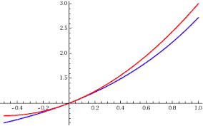
If our differential equation is not autonomous, the situation becomes a bit more involved. As a prototypical example let us investigate the differential equation
$$
\dot{x}=x^2-t^2 .
$$
It is of Riccati type and according to the previous section, it cannot be solved unless a particular solution can be found. But there does not seem to be a solution which can be easily guessed. (We will show later, in Problem 4.8, that it is explicitly solvable in terms of special functions.)

数学代写|常微分方程代写ordinary differential equation代考|Qualitative analysis of first-order periodic equations

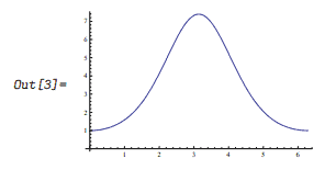
Some of the most interesting examples are periodic ones, where $f(t+1, x)=$ $f(t, x)$ (without loss we have assumed the period to be one). So let us consider the logistic growth model with a time dependent harvesting term
$$
\dot{x}(t)=(1-x(t)) x(t)-h \cdot(1-\sin (2 \pi t)),
$$
where $h \geq 0$ is some positive constant. In fact, we could replace $1-\sin (2 \pi t)$ by any nonnegative periodic function $g(t)$ and the analysis below will still hold.

The solutions corresponding to some initial conditions for $h=0.2$ are depicted below.

It looks like all solutions starting above some value $x_1$ converge to a periodic solution starting at some other value $x_2>x_1$, while solutions starting below $x_1$ diverge to $-\infty$.

They key idea is to look at the fate of an arbitrary initial value $x$ after precisely one period. More precisely, let us denote the solution which starts at the point $x$ at time $t=0$ by $\phi(t, x)$. Then we can introduce the Poincaré map via
$$
P(x)=\phi(1, x) .
$$
By construction, an initial condition $x_0$ will correspond to a periodic solution if and only if $x_0$ is a fixed point of the Poincaré map, $P\left(x_0\right)=x_0$. In fact, this follows from uniqueness of solutions of the initial value problem, since $\phi(t+1, x)$ again satisfies $\dot{x}=f(t, x)$ if $f(t+1, x)=f(t, x)$. So $\phi\left(t+1, x_0\right)=\phi\left(t, x_0\right)$ if and only if equality holds at the initial time $t=0$, that is, $\phi\left(1, x_0\right)=\phi\left(0, x_0\right)=x_0$.

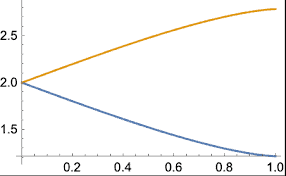
We begin by trying to compute the derivative of $P(x)$ as follows. Set
$$
\theta(t, x)=\frac{\partial}{\partial x} \phi(t, x)
$$
and differentiate the differential equation
$$
\dot{\phi}(t, x)=(1-\phi(t, x)) \phi(t, x)-h \cdot(1-\sin (2 \pi t)),
$$
with respect to $x$ (we will justify this step in Theorem 2.10). Then we obtain
$$
\dot{\theta}(t, x)=(1-2 \phi(t, x)) \theta(t, x)
$$
and assuming $\phi(t, x)$ is known we can use Problem $1.13$ to write down the solution
$$
\theta(t, x)=\exp \left(\int_0^t(1-2 \phi(s, x)) d s\right) .
$$

数学代写|常微分方程代写ordinary differential equation代考|MATH211

常微分方程代写

数学代写|常微分方程代写ordinary differential equation代考|Qualitative analysis of first-order equations

如前一节所述,只有极少数常微分方程是可明确解的。幸运的是,在许多情况下,不需要解决方案,只对解决方案 的一些定性方面感兴趣。例如,它是否停留在某个区域内,它看起来像大 $t$ ,ETC。
此外,即使在可以获得精确解的情况下,定性分析也可以比解的公式更好地概述行为。例如,考虑逻辑增长模型 (问题 1.16)
$$
\dot{x}(t)=(1-x(t)) x(t)-h,
$$
这可以通过变量分离来解决。为了获得概览,我们绘制相应的右侧 $f(x)=(1-x) x-h$ : 自从签到 $f(x)$ 告诉我 们解决方案将朝哪个方向发展,我们所要做的就是讨论 $f(x) !$ 为了 $0\frac{1}{4}$ 没有零点,所有解都 减少并收敛到 $-\infty$.
所以我们只要讨论 $f(x)$ ! 更一般地,对于一阶自主初始值问题(问题 1.27),我们有以下结果
$$
\dot{x}=f(x), \quad x(0)=x_0,
$$
在哪里 $f$ 是这样的解决方案是唯一的(例如 $f \in C^1$ ) 。
$(一)$ 如果 $f\left(x_0\right)=0$ ,然后 $x(t)=x_0$ 对所有人 $t$.
(ii) 如果 $f\left(x_0\right) \neq 0$ ,然后 $x(t)$ 收玫到左边的第一个零 $\left(f\left(x_0\right)<0\right)$ 分别对 $\left(f\left(x_0\right)>0\right)$ 的 $x_0$. 如果没有这样的 零,则解收敛到 $-\infty$ ,分别 $\infty$.
如果我们的微分方程不是自主的,情况就会变得更加复杂。作为一个典型的例子,让我们研究微分方程
$$
\dot{x}=x^2-t^2 .
$$
它是 Riccati 类型的,根据前面的部分,除非找到特定的解决方案,否则它无法解决。但似乎没有一个容易猜到的 解决方案。(我们将在后面的问题 $4.8$ 中证明,它可以用特殊函数显式解决。)

数学代写|常微分方程代写ordinary differential equation代考|Qualitative analysis of first-order periodic equations

一些最有趣的例子是周期性的,其中 $f(t+1, x)=f(t, x)$ (没有损失,我们假设周期为一)。因此,让我们考 虑具有时间相关收获项的逻辑增长模型
$$
\dot{x}(t)=(1-x(t)) x(t)-h \cdot(1-\sin (2 \pi t)),
$$
在哪里 $h \geq 0$ 是一些正常数。事实上,我们可以替换 $1-\sin (2 \pi t)$ 由任何非负周期函数 $g(t)$ 下面的分析仍然成 立。
对应于一些初始条件的解 $h=0.2$ 如下图所示。
看起来所有解决方案都从某个值开始 $x_1$ 收敛到从某个其他值开始的周期解 $x_2>x_1$ ,而解决方案从下面开始 $x_1$ 发 散到 $-\infty$.
他们的关键思想是查看任意初始值的命运 $x$ 怙好在一个时期之后。更准确地说,让我们表示从点开始的解决方案 $x$ 有时 $t=0$ 经过 $\phi(t, x)$. 然后我们可以通过
$$
P(x)=\phi(1, x) .
$$
通过构造,初始条件 $x_0$ 将对应于周期解当且仅当 $x_0$ 是庞加莱图的一个不动点, $P\left(x_0\right)=x_0$. 事实上,这源于初 始值问题的解的唯一性,因为 $\phi(t+1, x)$ 再次满足 $\dot{x}=f(t, x)$ 如果 $f(t+1, x)=f(t, x)$. 所以 $\phi\left(t+1, x_0\right)=\phi\left(t, x_0\right)$ 当且仅当等式在初始时间成立 $t=0$ ,那是, $\phi\left(1, x_0\right)=\phi\left(0, x_0\right)=x_0$.
我们首先尝试计算 $P(x)$ 如下。放
$$
\theta(t, x)=\frac{\partial}{\partial x} \phi(t, x)
$$
并微分方程
$$
\dot{\phi}(t, x)=(1-\phi(t, x)) \phi(t, x)-h \cdot(1-\sin (2 \pi t)),
$$
关于 $x$ (我们将在定理 $2.10$ 中证明这一步的合理性)。然后我们得到
$$
\dot{\theta}(t, x)=(1-2 \phi(t, x)) \theta(t, x)
$$
并假设 $\phi(t, x)$ 已知我们可以使用问题 $1.13$ 写下解决方案
$$
\theta(t, x)=\exp \left(\int_0^t(1-2 \phi(s, x)) d s\right) .
$$

统计代写请认准statistics-lab™. statistics-lab™为您的留学生涯保驾护航。

金融工程代写

金融工程是使用数学技术来解决金融问题。金融工程使用计算机科学、统计学、经济学和应用数学领域的工具和知识来解决当前的金融问题,以及设计新的和创新的金融产品。

非参数统计代写

非参数统计指的是一种统计方法,其中不假设数据来自于由少数参数决定的规定模型;这种模型的例子包括正态分布模型和线性回归模型。

广义线性模型代考

广义线性模型(GLM)归属统计学领域,是一种应用灵活的线性回归模型。该模型允许因变量的偏差分布有除了正态分布之外的其它分布。

术语 广义线性模型(GLM)通常是指给定连续和/或分类预测因素的连续响应变量的常规线性回归模型。它包括多元线性回归,以及方差分析和方差分析(仅含固定效应)。

有限元方法代写

有限元方法(FEM)是一种流行的方法,用于数值解决工程和数学建模中出现的微分方程。典型的问题领域包括结构分析、传热、流体流动、质量运输和电磁势等传统领域。

有限元是一种通用的数值方法,用于解决两个或三个空间变量的偏微分方程(即一些边界值问题)。为了解决一个问题,有限元将一个大系统细分为更小、更简单的部分,称为有限元。这是通过在空间维度上的特定空间离散化来实现的,它是通过构建对象的网格来实现的:用于求解的数值域,它有有限数量的点。边界值问题的有限元方法表述最终导致一个代数方程组。该方法在域上对未知函数进行逼近。[1] 然后将模拟这些有限元的简单方程组合成一个更大的方程系统,以模拟整个问题。然后,有限元通过变化微积分使相关的误差函数最小化来逼近一个解决方案。

tatistics-lab作为专业的留学生服务机构,多年来已为美国、英国、加拿大、澳洲等留学热门地的学生提供专业的学术服务,包括但不限于Essay代写,Assignment代写,Dissertation代写,Report代写,小组作业代写,Proposal代写,Paper代写,Presentation代写,计算机作业代写,论文修改和润色,网课代做,exam代考等等。写作范围涵盖高中,本科,研究生等海外留学全阶段,辐射金融,经济学,会计学,审计学,管理学等全球99%专业科目。写作团队既有专业英语母语作者,也有海外名校硕博留学生,每位写作老师都拥有过硬的语言能力,专业的学科背景和学术写作经验。我们承诺100%原创,100%专业,100%准时,100%满意。

随机分析代写


随机微积分是数学的一个分支,对随机过程进行操作。它允许为随机过程的积分定义一个关于随机过程的一致的积分理论。这个领域是由日本数学家伊藤清在第二次世界大战期间创建并开始的。

时间序列分析代写

随机过程,是依赖于参数的一组随机变量的全体,参数通常是时间。 随机变量是随机现象的数量表现,其时间序列是一组按照时间发生先后顺序进行排列的数据点序列。通常一组时间序列的时间间隔为一恒定值(如1秒,5分钟,12小时,7天,1年),因此时间序列可以作为离散时间数据进行分析处理。研究时间序列数据的意义在于现实中,往往需要研究某个事物其随时间发展变化的规律。这就需要通过研究该事物过去发展的历史记录,以得到其自身发展的规律。

回归分析代写

多元回归分析渐进(Multiple Regression Analysis Asymptotics)属于计量经济学领域,主要是一种数学上的统计分析方法,可以分析复杂情况下各影响因素的数学关系,在自然科学、社会和经济学等多个领域内应用广泛。

MATLAB代写

MATLAB 是一种用于技术计算的高性能语言。它将计算、可视化和编程集成在一个易于使用的环境中,其中问题和解决方案以熟悉的数学符号表示。典型用途包括:数学和计算算法开发建模、仿真和原型制作数据分析、探索和可视化科学和工程图形应用程序开发,包括图形用户界面构建MATLAB 是一个交互式系统,其基本数据元素是一个不需要维度的数组。这使您可以解决许多技术计算问题,尤其是那些具有矩阵和向量公式的问题,而只需用 C 或 Fortran 等标量非交互式语言编写程序所需的时间的一小部分。MATLAB 名称代表矩阵实验室。MATLAB 最初的编写目的是提供对由 LINPACK 和 EISPACK 项目开发的矩阵软件的轻松访问,这两个项目共同代表了矩阵计算软件的最新技术。MATLAB 经过多年的发展,得到了许多用户的投入。在大学环境中,它是数学、工程和科学入门和高级课程的标准教学工具。在工业领域,MATLAB 是高效研究、开发和分析的首选工具。MATLAB 具有一系列称为工具箱的特定于应用程序的解决方案。对于大多数 MATLAB 用户来说非常重要,工具箱允许您学习应用专业技术。工具箱是 MATLAB 函数(M 文件)的综合集合,可扩展 MATLAB 环境以解决特定类别的问题。可用工具箱的领域包括信号处理、控制系统、神经网络、模糊逻辑、小波、仿真等。

R语言代写问卷设计与分析代写
PYTHON代写回归分析与线性模型代写
MATLAB代写方差分析与试验设计代写
STATA代写机器学习/统计学习代写
SPSS代写计量经济学代写
EVIEWS代写时间序列分析代写
EXCEL代写深度学习代写
SQL代写各种数据建模与可视化代写

数学代写|常微分方程代写ordinary differential equation代考|MATH2410

如果你也在 怎样代写常微分方程ordinary differential equation这个学科遇到相关的难题,请随时右上角联系我们的24/7代写客服。

常微分方程是为一个或多个独立变量的函数及其导数定义的方程。y’=x+1是一个常微分方程的例子。

statistics-lab™ 为您的留学生涯保驾护航 在代写常微分方程ordinary differential equation方面已经树立了自己的口碑, 保证靠谱, 高质且原创的统计Statistics代写服务。我们的专家在代写常微分方程ordinary differential equation代写方面经验极为丰富,各种代写常微分方程ordinary differential equation相关的作业也就用不着说。

我们提供的常微分方程ordinary differential equation及其相关学科的代写,服务范围广, 其中包括但不限于:

  • Statistical Inference 统计推断
  • Statistical Computing 统计计算
  • Advanced Probability Theory 高等概率论
  • Advanced Mathematical Statistics 高等数理统计学
  • (Generalized) Linear Models 广义线性模型
  • Statistical Machine Learning 统计机器学习
  • Longitudinal Data Analysis 纵向数据分析
  • Foundations of Data Science 数据科学基础
数学代写|常微分方程代写ordinary differential equation代考|MATH2410

数学代写|常微分方程代写ordinary differential equation代考|First order autonomous equations

Let us look at the simplest (nontrivial) case of a first-order autonomous equation and let us try to find the solution starting at a certain point $x_0$ at time $t=0$ :
$$
\dot{x} f(x), \quad x(0) \quad x_0, \quad f \in C(\mathbb{R})
$$

We could of course also ask for the solution starting at $x_0$ at time $t_0$. However, once we have a solution $\phi(t)$ with $\phi(0)=x_0$, the solution $\psi(t)$ with $\psi\left(t_0\right)=x_0$ is given by a simple shift $\psi(t)=\phi\left(t-t_0\right)$ (this holds in fact for any autonomous equation – compare Problem 1.8).

This equation can be solved using a small ruse. If $f\left(x_0\right) \neq 0$, we can divide both sides by $f(x)$ and integrate both sides with respect to $t$ :
$$
\int_0^t \frac{\dot{x}(s) d s}{f(x(s))}=t \text {. }
$$
Abbreviating $F(x)=\int_{x_0}^x \frac{d y}{f(y)}$ we see that every solution $x(t)$ of $(1.20)$ must satisfy $F(x(t))=t$. Since $F(x)$ is strictly monotone near $x_0$, it can be inverted and we obtain a unique solution
$$
\phi(t)=F^{-1}(t), \quad \phi(0)=F^{-1}(0)=x_0,
$$
of our initial value problem. Here $F^{-1}(t)$ is the inverse map of $F(t)$.
Now let us look at the maximal interval of existence. If $f\left(x_0\right)>0$ (the case $f\left(x_0\right)<0$ follows analogously), then $f$ remains positive in some interval $\left(x_1, x_2\right)$ around $x_0$ by continuity. Define $T_{+}=\lim {x \uparrow x_2} F(x) \in(0, \infty], \quad$ respectively $\quad T{-}=\lim {x \downarrow x_1} F(x) \in[-\infty, 0)$. (1.23) Then $\phi \in C^1\left(\left(T{-}, T_{+}\right)\right)$and $$ \lim {t \uparrow T{+}} \phi(t)=x_2, \quad \text { respectively } \quad \lim {t \downarrow T{-}} \phi(t)=x_1 . $$ In particular, $\phi$ exists for all $t>0$ (resp. $t<0$ ) if and only if
$$
T_{+}=\int_{x_0}^{x_2} \frac{d y}{f(y)}=+\infty,
$$
that is, if $1 / f(x)$ is not integrable near $x_2$. Similarly, $\phi$ exists for all $t<0$ if and only if $1 / f(x)$ is not integrable near $x_1$.
Now let us look at some examples.

数学代写|常微分方程代写ordinary differential equation代考|Finding explicit solutions

We have seen in the previous section, that some differential equations can be solved explicitly. Unfortunately, there is no general recipe for solving a given differential equation. Moreover, finding explicit solutions is in general impossible unless the equation is of a particular form. In this section I will show you some classes of first-order equations which are explicitly solvable.
The general idea is to find a suitable change of variables which transforms the given equation into a solvable form. Hence we want to review this concept first. Given the point with coordinates $(t, x)$, we may change to new coordinates $(s, y)$ given by
$$
s=\sigma(t, x), \quad y=\eta(t, x) .
$$
Since we do not want to lose information, we require this transformation to be invertible.

A given function $\phi(t)$ will be transformed into a function $\psi(s)$ which has to be obtained by eliminating $t$ from
$$
s=\sigma(t, \phi(t)), \quad \psi=\eta(t, \phi(t)) .
$$
Unfortunately this will not always be possible (e.g., if we rotate the graph of a function in $\mathbb{R}^2$, the refiult might not be the graph of a function). To avoid this problem we restrict our attention to the special case of fiber preserving transformations
$$
s=\sigma(t), \quad y=\eta(t, x)
$$
(which map the fibers $t=$ const to the fibers $s=$ const). Denoting the inverse transform by
$$
t=\tau(s), \quad x=\xi(s, y),
$$
a straightforward application of the chain rule shows that $\phi(t)$ satisfies
$$
\dot{x}=f(t, x)
$$
if and only if $\psi(s)=\eta(\tau(s), \phi(\tau(s)))$ satisfies
$$
\dot{y}=\dot{\tau}\left(\frac{\partial \eta}{\partial t}(\tau, \xi)+\frac{\partial \eta}{\partial x}(\tau, \xi) f(\tau, \xi)\right),
$$
where $\tau=\tau(s)$ and $\xi=\xi(s, y)$.

数学代写|常微分方程代写ordinary differential equation代考|MATH2410

常微分方程代写

数学代写|常微分方程代写ordinary differential equation代考|First order autonomous equations

让我们看一下一阶自治方程的最简单 (非平凡) 情况,让我们尝试从某个点开始找到解 $x_0$ 有时 $t=0$ :
$$
\dot{x} f(x), \quad x(0) \quad x_0, \quad f \in C(\mathbb{R})
$$
我们当然也可以要求解决方案从 $x_0$ 有时 $t_0$. 但是,一旦我们有了解决方案 $\phi(t)$ 和 $\phi(0)=x_0$ ,解决方案 $\psi(t)$ 和 $\psi\left(t_0\right)=x_0$ 由一个简单的移位给出 $\psi(t)=\phi\left(t-t_0\right)$ (这实际上适用于任何自治方程一一比较问题 1.8) 。
这个方程可以用一个小技巧来解决。如果 $f\left(x_0\right) \neq 0$ ,我们可以将两边除以 $f(x)$ 并整合双方关于 $t$ :
$$
\int_0^t \frac{\dot{x}(s) d s}{f(x(s))}=t .
$$
缩写 $F(x)=\int_{x_0}^x \frac{d y}{f(y)}$ 我们看到每个解决方案 $x(t)$ 的 $(1.20)$ 必须满足 $F(x(t))=t$. 自从 $F(x)$ 附近是严格单调的 $x_0$ ,它可以被反转,我们得到一个唯一的解决方案
$$
\phi(t)=F^{-1}(t), \quad \phi(0)=F^{-1}(0)=x_0,
$$
我们的初值问题。这里 $F^{-1}(t)$ 是的逆映射 $F(t)$.
现在让我们看看存在的最大间隔。如果 $f\left(x_0\right)>0$ (案子 $f\left(x_0\right)<0$ 类似地遵循),然后 $f$ 在一段时间内保持积 极 $\left(x_1, x_2\right)$ 大约 $x_0$ 通过连续性。定义 $T_{+}=\lim x \uparrow x_2 F(x) \in(0, \infty]$, 分别 $T-=\lim x \downarrow x_1 F(x) \in[-\infty, 0)$. (1.23) 那么 $\phi \in C^1\left(\left(T-, T_{+}\right)\right)$和 $\lim t \uparrow T+\phi(t)=x_2, \quad$ respectively $\quad \lim t \downarrow T-\phi(t)=x_1$. 尤其是, $\phi$ 为所有人而存在 $t>0$ (分别。 $t<0$ ) 当且仅当
$$
T_{+}=\int_{x_0}^{x_2} \frac{d y}{f(y)}=+\infty
$$
也就是说,如果 $1 / f(x)$ 附近不可积 $x_2$. 相似地, $\phi$ 为所有人而存在 $t<0$ 当且仅当 $1 / f(x)$ 附近不可积 $x_1$. 现在让我们看一些例子。

数学代写|常微分方程代写ordinary differential equation代考|Finding explicit solutions

我们在上一节中已经看到,一些微分方程可以显式求解。不幸的是,没有解决给定微分方程的通用方法。此外,除 非方程具有特定形式,否则通常不可能找到明确的解。在本节中,我将向您展示一些明确可解的一阶方程。
总体思路是找到合适的变量变化,将给定方程转换为可解形式。因此,我们想先回顾一下这个概念。给定坐标点 $(t, x)$ ,我们可能会改变到新的坐标 $(s, y)$ 由
$$
s=\sigma(t, x), \quad y=\eta(t, x) .
$$
由于我们不想至失信息,因此我们要求这种转换是可逆的。
给定函数 $\phi(t)$ 将转化为函数 $\psi(s)$ 这必须通过消除来获得 $t$ 从
$$
s=\sigma(t, \phi(t)), \quad \psi=\eta(t, \phi(t)) .
$$
不幸的是,这并不总是可能的(例如,如果我们在 $\mathbb{R}^2$ ,结果可能不是函数图)。为了避免这个问题,我们将注意 力限制在纤维保留变换的特殊情况上
$$
s=\sigma(t), \quad y=\eta(t, x)
$$
(映射纤维 $t=$ const 到纤维 $s=$ 常量)。将逆变换表示为
$$
t=\tau(s), \quad x=\xi(s, y),
$$
链式法则的直接应用表明 $\phi(t)$ 满足
$$
\dot{x}=f(t, x)
$$
当且仅当 $\psi(s)=\eta(\tau(s), \phi(\tau(s)))$ 满足
$$
\dot{y}=\dot{\tau}\left(\frac{\partial \eta}{\partial t}(\tau, \xi)+\frac{\partial \eta}{\partial x}(\tau, \xi) f(\tau, \xi)\right),
$$
在哪里 $\tau=\tau(s)$ 和 $\xi=\xi(s, y)$.

统计代写请认准statistics-lab™. statistics-lab™为您的留学生涯保驾护航。

金融工程代写

金融工程是使用数学技术来解决金融问题。金融工程使用计算机科学、统计学、经济学和应用数学领域的工具和知识来解决当前的金融问题,以及设计新的和创新的金融产品。

非参数统计代写

非参数统计指的是一种统计方法,其中不假设数据来自于由少数参数决定的规定模型;这种模型的例子包括正态分布模型和线性回归模型。

广义线性模型代考

广义线性模型(GLM)归属统计学领域,是一种应用灵活的线性回归模型。该模型允许因变量的偏差分布有除了正态分布之外的其它分布。

术语 广义线性模型(GLM)通常是指给定连续和/或分类预测因素的连续响应变量的常规线性回归模型。它包括多元线性回归,以及方差分析和方差分析(仅含固定效应)。

有限元方法代写

有限元方法(FEM)是一种流行的方法,用于数值解决工程和数学建模中出现的微分方程。典型的问题领域包括结构分析、传热、流体流动、质量运输和电磁势等传统领域。

有限元是一种通用的数值方法,用于解决两个或三个空间变量的偏微分方程(即一些边界值问题)。为了解决一个问题,有限元将一个大系统细分为更小、更简单的部分,称为有限元。这是通过在空间维度上的特定空间离散化来实现的,它是通过构建对象的网格来实现的:用于求解的数值域,它有有限数量的点。边界值问题的有限元方法表述最终导致一个代数方程组。该方法在域上对未知函数进行逼近。[1] 然后将模拟这些有限元的简单方程组合成一个更大的方程系统,以模拟整个问题。然后,有限元通过变化微积分使相关的误差函数最小化来逼近一个解决方案。

tatistics-lab作为专业的留学生服务机构,多年来已为美国、英国、加拿大、澳洲等留学热门地的学生提供专业的学术服务,包括但不限于Essay代写,Assignment代写,Dissertation代写,Report代写,小组作业代写,Proposal代写,Paper代写,Presentation代写,计算机作业代写,论文修改和润色,网课代做,exam代考等等。写作范围涵盖高中,本科,研究生等海外留学全阶段,辐射金融,经济学,会计学,审计学,管理学等全球99%专业科目。写作团队既有专业英语母语作者,也有海外名校硕博留学生,每位写作老师都拥有过硬的语言能力,专业的学科背景和学术写作经验。我们承诺100%原创,100%专业,100%准时,100%满意。

随机分析代写


随机微积分是数学的一个分支,对随机过程进行操作。它允许为随机过程的积分定义一个关于随机过程的一致的积分理论。这个领域是由日本数学家伊藤清在第二次世界大战期间创建并开始的。

时间序列分析代写

随机过程,是依赖于参数的一组随机变量的全体,参数通常是时间。 随机变量是随机现象的数量表现,其时间序列是一组按照时间发生先后顺序进行排列的数据点序列。通常一组时间序列的时间间隔为一恒定值(如1秒,5分钟,12小时,7天,1年),因此时间序列可以作为离散时间数据进行分析处理。研究时间序列数据的意义在于现实中,往往需要研究某个事物其随时间发展变化的规律。这就需要通过研究该事物过去发展的历史记录,以得到其自身发展的规律。

回归分析代写

多元回归分析渐进(Multiple Regression Analysis Asymptotics)属于计量经济学领域,主要是一种数学上的统计分析方法,可以分析复杂情况下各影响因素的数学关系,在自然科学、社会和经济学等多个领域内应用广泛。

MATLAB代写

MATLAB 是一种用于技术计算的高性能语言。它将计算、可视化和编程集成在一个易于使用的环境中,其中问题和解决方案以熟悉的数学符号表示。典型用途包括:数学和计算算法开发建模、仿真和原型制作数据分析、探索和可视化科学和工程图形应用程序开发,包括图形用户界面构建MATLAB 是一个交互式系统,其基本数据元素是一个不需要维度的数组。这使您可以解决许多技术计算问题,尤其是那些具有矩阵和向量公式的问题,而只需用 C 或 Fortran 等标量非交互式语言编写程序所需的时间的一小部分。MATLAB 名称代表矩阵实验室。MATLAB 最初的编写目的是提供对由 LINPACK 和 EISPACK 项目开发的矩阵软件的轻松访问,这两个项目共同代表了矩阵计算软件的最新技术。MATLAB 经过多年的发展,得到了许多用户的投入。在大学环境中,它是数学、工程和科学入门和高级课程的标准教学工具。在工业领域,MATLAB 是高效研究、开发和分析的首选工具。MATLAB 具有一系列称为工具箱的特定于应用程序的解决方案。对于大多数 MATLAB 用户来说非常重要,工具箱允许您学习应用专业技术。工具箱是 MATLAB 函数(M 文件)的综合集合,可扩展 MATLAB 环境以解决特定类别的问题。可用工具箱的领域包括信号处理、控制系统、神经网络、模糊逻辑、小波、仿真等。

R语言代写问卷设计与分析代写
PYTHON代写回归分析与线性模型代写
MATLAB代写方差分析与试验设计代写
STATA代写机器学习/统计学习代写
SPSS代写计量经济学代写
EVIEWS代写时间序列分析代写
EXCEL代写深度学习代写
SQL代写各种数据建模与可视化代写

数学代写|常微分方程代写ordinary differential equation代考|MATH3331

如果你也在 怎样代写常微分方程ordinary differential equation这个学科遇到相关的难题,请随时右上角联系我们的24/7代写客服。

常微分方程是为一个或多个独立变量的函数及其导数定义的方程。y’=x+1是一个常微分方程的例子。

statistics-lab™ 为您的留学生涯保驾护航 在代写常微分方程ordinary differential equation方面已经树立了自己的口碑, 保证靠谱, 高质且原创的统计Statistics代写服务。我们的专家在代写常微分方程ordinary differential equation代写方面经验极为丰富,各种代写常微分方程ordinary differential equation相关的作业也就用不着说。

我们提供的常微分方程ordinary differential equation及其相关学科的代写,服务范围广, 其中包括但不限于:

  • Statistical Inference 统计推断
  • Statistical Computing 统计计算
  • Advanced Probability Theory 高等概率论
  • Advanced Mathematical Statistics 高等数理统计学
  • (Generalized) Linear Models 广义线性模型
  • Statistical Machine Learning 统计机器学习
  • Longitudinal Data Analysis 纵向数据分析
  • Foundations of Data Science 数据科学基础
数学代写|常微分方程代写ordinary differential equation代考|MATH3331

数学代写|常微分方程代写ordinary differential equation代考|Newton’s equations

Let us begin with an example from physics. In classical mechanics a particle is described by a point in space whose location is given by a function

The derivative of this function with respect to time is the velocity of the particle
$$
v=\dot{x}: \mathbb{R} \rightarrow \mathbb{R}^3
$$
and the derivative of the velocity is the acceleration
$$
a=\dot{v}: \mathbb{R} \rightarrow \mathbb{R}^3 .
$$
In such a model the particle is usually moving in an external force field
$$
F: \mathbb{R}^3 \rightarrow \mathbb{R}^3
$$
which exerts a force $F(x)$ on the particle at $x$. The Newton’s second law states that, at each point $x$ in space, the force acting on the particle must be equal to the acceleration times the mass $m$ (a positive constant) of the particle, that is,
$$
m \ddot{x}(t)=F(x(t)), \quad \text { for all } t \in \mathbb{R} .
$$
Such a relation between a function $x(t)$ and its derivatives is called a differential equation. Equation (1.5) is of second order since the highest derivative is of second degree. More precisely, we have a system of differential equations since there is one for each coordinate direction.

In our case $x$ is called the dependent and $t$ is called the independent variable. It is also possible to increase the number of dependent variables by adding $v$ to the dependent variables and considering $(x, v) \in \mathbb{R}^6$. The advantage is, that we now have a first-order system
$$
\begin{aligned}
\dot{x}(t) &=v(t) \
\dot{v}(t) &=\frac{1}{m} F(x(t)) .
\end{aligned}
$$
This form is often better suited for theoretical investigations.
For given force $F$ one wants to find solutions, that is functions $x(t)$ that satisfy (1.5) (respectively (1.6)). To be more specific, let us look at the motion of a stone falling towards the earth. In the vicinity of the surface of the earth, the gravitational force acting on the stone is approximately constant and given by
$$
F(x)=-m g\left(\begin{array}{l}
0 \
0 \
1
\end{array}\right) \text {. }
$$

数学代写|常微分方程代写ordinary differential equation代考|Classification of differential equations

Let $U \subseteq \mathbb{R}^m, V \subseteq \mathbb{R}^n$ and $k \in \mathbb{N}_0$. Then $C^k(U, V)$ denotes the set of functions $U \rightarrow V$ having continuous derivatives up to order $k$. In addition, we will abbreviate $C(U, V)=C^0(U, V)$ and $C^k(U)=C^k(U, \mathbb{R})$.

A classical ordinary differential equation (ODE) is a relation of the form
$$
F\left(t, x, x^{(1)}, \ldots, x^{(k)}\right)=0
$$
for the unknown function $x \in C^k(J), J \subseteq \mathbb{R}$. Here $F \in C(U)$ with $U$ an open subset of $\mathbb{R}^{k+2}$ and
$$
x^{(k)}(t)=\frac{d^k x(t)}{d t^k}, \quad k \in \mathbb{N}_0,
$$
are the ordinary derivatives of $x$. One frequently calls $t$ the independent and $x$ the dependent variable. The highest derivative appearing in $F$ is called the order of the differential equation. A solution of the ODE (1.12) is a function $\phi \in C^k(I)$, where $I \subseteq J$ is an interval, such that
$$
F\left(t, \phi(t), \phi^{(1)}(t), \ldots, \phi^{(k)}(t)\right)=0, \quad \text { for all } t \in I \text {. }
$$
This implicitly implies $\left(t, \phi(t), \phi^{(1)}(t), \ldots, \phi^{(k)}(t)\right) \in U$ for all $t \in I$.
Unfortunately there is not too much one can say about general differential equations in the above form (1.12). Hence we will assume that one can solve $F$ for the highest derivative, resulting in a differential equation of the form
$$
x^{(k)}=f\left(t, x, x^{(1)}, \ldots, x^{(k-1)}\right)
$$
By the implicit function theorem this can be done at least locally near some point $(t, y) \in U$ if the partial derivative with respect to the highest derivative does not vanish at that point, $\frac{\partial F}{\partial y_k}(t, y) \neq 0$. This is the type of differential equations we will consider from now on.

数学代写|常微分方程代写ordinary differential equation代考|MATH3331

常微分方程代写

数学代写|常微分方程代写ordinary differential equation代考|Newton’s equations

让我们从物理学中的一个例子开始。在经典力学中,粒子由空间中的一个点来描述,该点的位置由函数给出
这个函数对时间的导数就是粒子的速度
$$
v=\dot{x}: \mathbb{R} \rightarrow \mathbb{R}^3
$$
速度的导数就是加速度
$$
a=\dot{v}: \mathbb{R} \rightarrow \mathbb{R}^3 .
$$
在这样的模型中,粒子通常在外力场中运动
$$
F: \mathbb{R}^3 \rightarrow \mathbb{R}^3
$$
施加力 $F(x)$ 在粒子上 $x$. 牛顿第二定律指出,在每一点 $x$ 在太空中,作用在粒子上的力必须等于加速度乘以质量 $m$ 粒子的 (正常数),即 $m \ddot{x}(t)=F(x(t)), \quad$ for all $t \in \mathbb{R}$.
函数之间的这种关系 $x(t)$ 其导数称为微分方程。方程 $(1.5)$ 是二阶的,因为最高导数是二阶的。更准确地说,我 们有一个微分方程系统,因为每个坐标方向都有一个。
在我们的例子中 $x$ 被称为依赖和 $t$ 称为自变量。也可以通过添加来增加因变量的数量 $v$ 到因变量并考虑 $(x, v) \in \mathbb{R}^6$. 优点是,我们现在有一个一阶系统
$$
\dot{x}(t)=v(t) \dot{v}(t) \quad=\frac{1}{m} F(x(t)) .
$$
这种形式通常更适合理论研究。
对于给定的力 $F$ 一个人想找到解决方案,那就是函数 $x(t)$ 满足 (1.5) (分别为 (1.6)) 。更具体地说,让我们看 一下石头落向地球的运动。在地球表面附近,作用在石头上的重力近似恒定,由下式给出
$$
F(x)=-m g\left(\begin{array}{llll}
0 & 0 & 1
\end{array}\right) .
$$

数学代写|常微分方程代写ordinary differential equation代考|Classification of differential equations

让 $U \subseteq \mathbb{R}^m, V \subseteq \mathbb{R}^n$ 和 $k \in \mathbb{N}_0$. 然后 $C^k(U, V)$ 表示函数集 $U \rightarrow V$ 有连续的衍生品订单 $k$. 此外,我们将缩写 $C(U, V)=C^0(U, V)$ 和 $C^k(U)=C^k(U, \mathbb{R})$.
经典常微分方程 (ODE) 是以下形式的关系
$$
F\left(t, x, x^{(1)}, \ldots, x^{(k)}\right)=0
$$
对于末知函数 $x \in C^k(J), J \subseteq \mathbb{R}$. 这里 $F \in C(U)$ 和 $U$ 的一个开放子集 $\mathbb{R}^{k+2}$ 和
$$
x^{(k)}(t)=\frac{d^k x(t)}{d t^k}, \quad k \in \mathbb{N}_0,
$$
是的普通导数 $x$.一个经常打电话 $t$ 独立和 $x$ 因变量。出现的最高导数 $F$ 称为微分方程的阶数。ODE (1.12) 的解是一 个函数 $\phi \in C^k(I)$ , 在哪里 $I \subseteq J$ 是一个区间,使得
$$
F\left(t, \phi(t), \phi^{(1)}(t), \ldots, \phi^{(k)}(t)\right)=0, \quad \text { for all } t \in I .
$$
这隐含地暗示 $\left(t, \phi(t), \phi^{(1)}(t), \ldots, \phi^{(k)}(t)\right) \in U$ 对所有人 $t \in I$.
不幸的是,对于上述形式 (1.12) 的一般溦分方程,没有太多可以说的。因此,我们假设可以解决 $F$ 对于最高导数, 得到形式为的微分方程
$$
x^{(k)}=f\left(t, x, x^{(1)}, \ldots, x^{(k-1)}\right)
$$
根据隐函数定理,这至少可以在某个点附近局部完成 $(t, y) \in U$ 如果关于最高导数的偏导数在该点没有消失, $\frac{\partial F}{\partial y_k}(t, y) \neq 0$. 这是我们从现在开始考虑的微分方程类型。

统计代写请认准statistics-lab™. statistics-lab™为您的留学生涯保驾护航。

金融工程代写

金融工程是使用数学技术来解决金融问题。金融工程使用计算机科学、统计学、经济学和应用数学领域的工具和知识来解决当前的金融问题,以及设计新的和创新的金融产品。

非参数统计代写

非参数统计指的是一种统计方法,其中不假设数据来自于由少数参数决定的规定模型;这种模型的例子包括正态分布模型和线性回归模型。

广义线性模型代考

广义线性模型(GLM)归属统计学领域,是一种应用灵活的线性回归模型。该模型允许因变量的偏差分布有除了正态分布之外的其它分布。

术语 广义线性模型(GLM)通常是指给定连续和/或分类预测因素的连续响应变量的常规线性回归模型。它包括多元线性回归,以及方差分析和方差分析(仅含固定效应)。

有限元方法代写

有限元方法(FEM)是一种流行的方法,用于数值解决工程和数学建模中出现的微分方程。典型的问题领域包括结构分析、传热、流体流动、质量运输和电磁势等传统领域。

有限元是一种通用的数值方法,用于解决两个或三个空间变量的偏微分方程(即一些边界值问题)。为了解决一个问题,有限元将一个大系统细分为更小、更简单的部分,称为有限元。这是通过在空间维度上的特定空间离散化来实现的,它是通过构建对象的网格来实现的:用于求解的数值域,它有有限数量的点。边界值问题的有限元方法表述最终导致一个代数方程组。该方法在域上对未知函数进行逼近。[1] 然后将模拟这些有限元的简单方程组合成一个更大的方程系统,以模拟整个问题。然后,有限元通过变化微积分使相关的误差函数最小化来逼近一个解决方案。

tatistics-lab作为专业的留学生服务机构,多年来已为美国、英国、加拿大、澳洲等留学热门地的学生提供专业的学术服务,包括但不限于Essay代写,Assignment代写,Dissertation代写,Report代写,小组作业代写,Proposal代写,Paper代写,Presentation代写,计算机作业代写,论文修改和润色,网课代做,exam代考等等。写作范围涵盖高中,本科,研究生等海外留学全阶段,辐射金融,经济学,会计学,审计学,管理学等全球99%专业科目。写作团队既有专业英语母语作者,也有海外名校硕博留学生,每位写作老师都拥有过硬的语言能力,专业的学科背景和学术写作经验。我们承诺100%原创,100%专业,100%准时,100%满意。

随机分析代写


随机微积分是数学的一个分支,对随机过程进行操作。它允许为随机过程的积分定义一个关于随机过程的一致的积分理论。这个领域是由日本数学家伊藤清在第二次世界大战期间创建并开始的。

时间序列分析代写

随机过程,是依赖于参数的一组随机变量的全体,参数通常是时间。 随机变量是随机现象的数量表现,其时间序列是一组按照时间发生先后顺序进行排列的数据点序列。通常一组时间序列的时间间隔为一恒定值(如1秒,5分钟,12小时,7天,1年),因此时间序列可以作为离散时间数据进行分析处理。研究时间序列数据的意义在于现实中,往往需要研究某个事物其随时间发展变化的规律。这就需要通过研究该事物过去发展的历史记录,以得到其自身发展的规律。

回归分析代写

多元回归分析渐进(Multiple Regression Analysis Asymptotics)属于计量经济学领域,主要是一种数学上的统计分析方法,可以分析复杂情况下各影响因素的数学关系,在自然科学、社会和经济学等多个领域内应用广泛。

MATLAB代写

MATLAB 是一种用于技术计算的高性能语言。它将计算、可视化和编程集成在一个易于使用的环境中,其中问题和解决方案以熟悉的数学符号表示。典型用途包括:数学和计算算法开发建模、仿真和原型制作数据分析、探索和可视化科学和工程图形应用程序开发,包括图形用户界面构建MATLAB 是一个交互式系统,其基本数据元素是一个不需要维度的数组。这使您可以解决许多技术计算问题,尤其是那些具有矩阵和向量公式的问题,而只需用 C 或 Fortran 等标量非交互式语言编写程序所需的时间的一小部分。MATLAB 名称代表矩阵实验室。MATLAB 最初的编写目的是提供对由 LINPACK 和 EISPACK 项目开发的矩阵软件的轻松访问,这两个项目共同代表了矩阵计算软件的最新技术。MATLAB 经过多年的发展,得到了许多用户的投入。在大学环境中,它是数学、工程和科学入门和高级课程的标准教学工具。在工业领域,MATLAB 是高效研究、开发和分析的首选工具。MATLAB 具有一系列称为工具箱的特定于应用程序的解决方案。对于大多数 MATLAB 用户来说非常重要,工具箱允许您学习应用专业技术。工具箱是 MATLAB 函数(M 文件)的综合集合,可扩展 MATLAB 环境以解决特定类别的问题。可用工具箱的领域包括信号处理、控制系统、神经网络、模糊逻辑、小波、仿真等。

R语言代写问卷设计与分析代写
PYTHON代写回归分析与线性模型代写
MATLAB代写方差分析与试验设计代写
STATA代写机器学习/统计学习代写
SPSS代写计量经济学代写
EVIEWS代写时间序列分析代写
EXCEL代写深度学习代写
SQL代写各种数据建模与可视化代写