如果你也在 怎样代写组合优化Combinatorial optimization这个学科遇到相关的难题，请随时右上角联系我们的24/7代写客服。

组合优化是处于组合学和理论计算机科学前沿的一个新兴领域，旨在使用组合技术解决离散优化问题。离散优化问题旨在从一个有限的可能性集合中确定可能的最佳解决方案。

组合优化是数学优化的一个子领域，包括从一个有限的对象集合中找到一个最佳对象，其中可行的解决方案的集合是离散的或可以减少到一个离散集合。典型的组合优化问题是旅行推销员问题（”TSP”）、最小生成树问题（”MST”）和结囊问题。在许多这样的问题中，如前面提到的问题，穷举搜索是不可行的，因此必须采用能迅速排除大部分搜索空间的专门算法或近似算法来代替。

statistics-lab™ 为您的留学生涯保驾护航 在代写组合优化Combinatorial optimization方面已经树立了自己的口碑, 保证靠谱, 高质且原创的统计Statistics代写服务。我们的专家在代写组合优化Combinatorial optimization代写方面经验极为丰富，各种代写组合优化Combinatorial optimization相关的作业也就用不着说。

我们提供的组合优化Combinatorial optimization及其相关学科的代写，服务范围广, 其中包括但不限于:

• Statistical Inference 统计推断
• Statistical Computing 统计计算
• Advanced Probability Theory 高等概率论
• Advanced Mathematical Statistics 高等数理统计学
• (Generalized) Linear Models 广义线性模型
• Statistical Machine Learning 统计机器学习
• Longitudinal Data Analysis 纵向数据分析
• Foundations of Data Science 数据科学基础

数学代写|组合优化代写Combinatorial optimization代考|k-edge-connected Spanning Subgraph Polyhedron

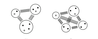
The dominant of a polyhedron $P$ is $\operatorname{dom}(P)={x: x=y+z$, for $y \in P$ and $z \geq \mathbf{0}}$. Note that $P_{k}(G)$ is the dominant of the convex hull of all $k$-edgeconnected spanning subgraphs of $G$ that have each edge taken at most $k$ times. Since the dominant of a polyhedron is a polyhedron, $P_{k}(G)$ is a polyhedron even though it is the convex hull of an infinite number of points.

From now on, $k \geq 2$. Didi Biha and Mahjoub (1996) gave a complete description of $P_{k}(G)$ for all $k$, when $G$ is series-parallel.

Theorem 2. Let $G$ be a series-parallel graph and $k$ be a positive integer. Then, when $k$ is even, $P_{k}(G)$ is described by:
(1) $\left{\begin{array}{l}x(D) \geq k \text { for all cuts } D \text { of } G, \ x \geq 0\end{array}\right.$
and when $k$ is odd, $P_{k}(G)$ is described by:
(2) $\left{\begin{array}{l}x(M) \geq \frac{k+1}{2} d_{M}-1 \text { for all multicuts } M \text { of } G, \ x \geq 0 .\end{array}\right.$
The incidence vector of a family $F$ of $E$ is the vector $\chi^{F}$ of $\mathbb{Z}^{E}$ such that $e$ ‘s coordinate is the multiplicity of $e$ in $F$ for all $e$ in $E$. Since there is a bijection between families and their incidence vectors, we will often use the same terminology for both. Since the incidence vector of a multicut $\delta\left(V_{1}, \ldots, V_{d_{M}}\right)$ is the half-sum of the incidence vectors of the bonds $\delta\left(V_{1}\right), \ldots, \delta\left(V_{d_{M}}\right)$, we can deduce an alternative description of $P_{2 h}(G)$.

Corollary 1. Let $G$ be a series-parallel graph and $k$ be a positive even integer. Then $P_{k}(G)$ is described by:
$$
\left{\begin{array}{l}
x(M) \geq \frac{k}{2} d_{M} \text { for all multicuts } M \text { of } G, \
x \geq \mathbf{0} .
\end{array}\right.
$$
We call constraints (2a) and (3a) partition constraints. A multicut $M$ is tight for a point of $P_{k}(G)$ if this point satisfies with equality the partition constraint (2a) (resp. (3a)) associated with $M$ when $k$ is odd (resp. even). Moreover, $M$ is tight for a face $F$ of $P_{k}(G)$ if it is tight for all the points of $F$.

The following results give some insight on the structure of tight multicuts.
Theorem 3 (Didi Biha and Mahjoub (1996)). Let $k>1$ be odd, let $x$ be a point of $P_{k}(G)$, and let $M=\delta\left(V_{1}, \ldots, V_{d_{M}}\right)$ be a multicut tight for $x$. Then, the following hold:
(i) if $d_{M} \geq 3$, then $x\left(\delta\left(V_{i}\right) \cap \delta\left(V_{j}\right)\right) \leq \frac{k+1}{2}$ for all $i \neq j \in\left{1, \ldots, d_{M}\right}$.
(ii) $G \backslash V_{i}$ is connected for all $i=1, \ldots, d_{M}$.
Observation 4. Let $M$ be a multicut of $G$ strictly containing $\delta(v)={f, g}$. If $M$ is tight for a point of $P_{k}(G)$, then both $M \backslash f$ and $M \backslash g$ are multicuts of $G$ of order $d_{M}-1$.

Chopra (1994) gave sufficient conditions for an inequality to be facet defining. The following proposition is a direct consequence of (Chopra 1994, Theorem 2.4).

数学代写|组合优化代写Combinatorial optimization代考|Box-TDIness of Pk

In this section we show that, for $k \geq 2, P_{k}(G)$ is a box-TDI polyhedron if and only if $G$ is series-parallel.

When $k \geq 2, P_{k}(G)$ is not box-TDI for all graphs as stated by the following lemma.

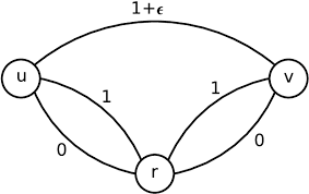
Lemma 1. For $k \geq 2$, if $G=(V, E)$ contains a $K_{4}$-minor, then $P_{k}(G)$ is not box-TDI.

Proof. When $k$ is odd, Proposition 2 shows that there exists a facet-defining inequality that is described by a non equimodular matrix. Thus, $P_{k}(G)$ is not box-TDI by Statement (ii) of Theorem 1 .

We now prove the case when $k$ is even. Since $G$ is connected and has a $K_{4^{-}}$ minor, there exists a partition $\left{V_{1}, \ldots, V_{4}\right}$ of $V$ such that $G\left[V_{i}\right]$ is connected and $\delta\left(V_{i}, V_{j}\right) \neq \emptyset$ for all $i<j \in{1, \ldots, 4}$. We prove that the matrix $T$ whose three rows are $\chi^{\delta\left(V_{i}\right)}$ for $i=1,2,3$ is a face-defining matrix for $P_{k}(G)$ which is not equimodular. This will end the proof by Statement (ii) of Theorem 1 .

Let $e_{i j}$ be an edge in $\delta\left(V_{i}, V_{j}\right)$ for all $i<j \in{1, \ldots, 4}$. The submatrix of $T$ formed by the columns associated with edges $e_{i j}$ is the following:

The matrix $T$ is not equimodular as the first three columns form a matrix of determinant $-2$ whereas the last three ones have determinant 1 .

To show that $T$ is face-defining, we exhibit $|E|-2$ affinely independent points of $P_{k}(G)$ satisfying the partition constraint (3a) associated with the multicut $\delta\left(V_{i}\right)$, that is, $x\left(\delta\left(V_{i}\right)\right)=k$, for $i=1,2,3$.

Let $D_{1}=\left{e_{12}, e_{14}, e_{23}, e_{34}\right}, D_{2}=\left{e_{12}, e_{13}, e_{24}, e_{34}\right}, D_{3}=\left{e_{13}, e_{14}, e_{23}, e_{24}\right}$ and $D_{4}=\left{e_{14}, e_{24}, e_{34}\right}$. First, we define the points $S_{j}=\sum_{i=1}^{4} k \chi^{E\left[V_{i}\right]}+\frac{k}{2} \chi^{D_{j}}$, for $j=1,2,3$, and $S_{4}=\sum_{i=1}^{4} k \chi^{E\left[V_{i}\right]}+k \chi^{D_{4}}$. Note that they are affinely independent.
Now, for each edge $e \notin\left{e_{12}, e_{13}, e_{14}, e_{23}, e_{24}, e_{34}\right}$, we construct the point $S_{c}$ as follows. When $e \in E\left[V_{i}\right]$ for some $i=1, \ldots, 4$, we define $S_{c}=S_{4}+\chi^{e}$. Adding the point $S_{e}$ maintains affine independence as $S_{e}$ is the only point not satisfying $x_{e}=k$. When $e \in \delta\left(V_{i}, V_{j}\right)$ for some $i, j$, we define $S_{e}=S_{\ell}-\chi^{e_{i j}}+\chi^{e}$, where $S_{\ell}$ is $S_{1}$ if $e \in \delta\left(V_{1}, V_{4}\right) \cup \delta\left(V_{2}, V_{3}\right)$ and $S_{2}$ otherwise. Affine independence comes because $S_{e}$ is the only point involving $e$.

数学代写|组合优化代写Combinatorial optimization代考|TDI Systems for Pk

Let $G$ be a series-parallel graph. In this section, we study the total dual integrality of systems describing $P_{k}(G)$. Due to length limitation, some of the proofs of the results below are omitted. They can be found in the appendix.

The following result characterizes series-parallel graphs in terms of TDIness of System (2).

Theorem 6. For $k>1$ odd and integer, System (2) is TDI if and only if $G$ is series-parallel.

Proof (sketch). We first prove that if $G$ is not series-parallel, then System (2) is not TDI. Indeed, every TDI system with integer right-hand side describes an integer polyhedron (Edmonds and Giles, 1977 ), but, when $G$ has a $K_{4}$-minor, System (2) describes a noninteger polyhedron (Chopra, 1994).

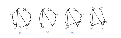
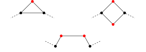
Let us sketch the other direction of the proof, that is, when the graph is series-parallel. We proceed by contradiction and consider a minimal counterexample $G$. First, we show that $G$ is simple and 2-connected. Then, we show that $G$ contains none of the following configurations.

Since the red vertices in the figure above have degree 2 in $G$, this contradicts Proposition $1 .$

For $k>1$, by Theorem $5, P_{k}(G)$ is a box-TDI polyhedron if and only if $G$ is series-parallel. Together with (Cook 1986, Corollary 2.5), this implies the following.

Corollary 2. For $k>1$ odd and integer, System (2) is box-TDI if and only if $G$ is series-parallel.The following theorem gives a TDI system for $P_{k}(G)$ when $G$ is series-parallel and $k$ is even.

组合优化代写

数学代写|组合优化代写Combinatorial optimization代考|k-edge-connected Spanning Subgraph Polyhedron

多面体的占优磷是dom⁡(磷)=X:X=是+和$,F这r$是∈磷$一种nd$和≥0. 注意磷ķ(G)是所有凸包的主导ķ-edgeconnected 的跨越子图G每条边最多取ķ次。由于多面体的主导是多面体，磷ķ(G)是一个多面体，尽管它是无限个点的凸包。

今后，ķ≥2. Didi Biha 和 Mahjoub (1996) 给出了完整的描述磷ķ(G)对全部ķ， 什么时候G是串并联的。

定理 2. 让G是一个串并图并且ķ为正整数。那么，当ķ甚至，磷ķ(G)描述为：
(1) $\left{X(D)≥ķ 对于所有削减 D 的 G, X≥0\对。一种nd在H和nķ一世s这dd,P_{k}(G)一世sd和sCr一世b和db是:(2)\剩下{X(米)≥ķ+12d米−1 对于所有多切 米 的 G, X≥0.\对。吨H和一世nC一世d和nC和在和C吨这r这F一种F一种米一世l是F这F和一世s吨H和在和C吨这r\chi^{F}这F\mathbb{Z}^{E}s在CH吨H一种吨和‘sC这这rd一世n一种吨和一世s吨H和米在l吨一世pl一世C一世吨是这F和一世nFF这r一种ll和一世n和.小号一世nC和吨H和r和一世s一种b一世j和C吨一世这nb和吨在和和nF一种米一世l一世和s一种nd吨H和一世r一世nC一世d和nC和在和C吨这rs,在和在一世ll这F吨和n在s和吨H和s一种米和吨和r米一世n这l这G是F这rb这吨H.小号一世nC和吨H和一世nC一世d和nC和在和C吨这r这F一种米在l吨一世C在吨\delta\left(V_{1}, \ldots, V_{d_{M}}\right)一世s吨H和H一种lF−s在米这F吨H和一世nC一世d和nC和在和C吨这rs这F吨H和b这nds\delta\left(V_{1}\right), \ldots, \delta\left(V_{d_{M}}\right),在和C一种nd和d在C和一种n一种l吨和rn一种吨一世在和d和sCr一世p吨一世这n这FP_{2 h}(G)$。

推论 1. 让G是一个串并图并且ķ为正偶数。然后磷ķ(G)描述为：
$$
\left{X(米)≥ķ2d米 对于所有多切 米 的 G, X≥0.\对。
$$
我们称约束 (2a) 和 (3a) 分区约束。多切米有点紧磷ķ(G)如果这一点满足相等的分区约束 (2a) (resp. (3a))米什么时候ķ是奇数（分别是偶数）。而且，米脸很紧F的磷ķ(G)如果它对所有点都很紧F.

以下结果对紧密多剪辑的结构提供了一些见解。
定理 3 (Didi Biha 和 Mahjoub (1996))。让ķ>1奇怪，让X成为一个点磷ķ(G)， 然后让米=d(在1,…,在d米)是一个多切紧X. 然后，以下成立：
（i）如果d米≥3， 然后X(d(在一世)∩d(在j))≤ķ+12对全部i \neq j \in\left{1, \ldots, d_{M}\right}i \neq j \in\left{1, \ldots, d_{M}\right}.
(二)G∖在一世为所有人连接一世=1,…,d米.
观察 4. 让米多选G严格包含d(在)=F,G. 如果米有点紧磷ķ(G), 那么两者米∖F和米∖G是多切G有秩序的d米−1.

Chopra (1994) 给出了定义一个不等式的充分条件。以下命题是 (Chopra 1994, Theorem 2.4) 的直接结果。

数学代写|组合优化代写Combinatorial optimization代考|Box-TDIness of Pk

在本节中，我们表明，对于ķ≥2,磷ķ(G)是一个盒 TDI 多面体当且仅当G是串并联的。

什么时候ķ≥2,磷ķ(G)不是以下引理所述的所有图的 box-TDI。

引理 1. 对于ķ≥2， 如果G=(在,和)包含一个ķ4-次要，然后磷ķ(G)不是box-TDI。

证明。什么时候ķ很奇怪，命题 2 表明存在一个由非等模矩阵描述的刻面定义不等式。因此，磷ķ(G)不是由定理 1 的陈述 (ii) 得出的 box-TDI。

我们现在证明当ķ甚至。自从G已连接并具有ķ4−次要，存在分区\left{V_{1}, \ldots, V_{4}\right}\left{V_{1}, \ldots, V_{4}\right}的在这样G[在一世]已连接并且d(在一世,在j)≠∅对全部一世<j∈1,…,4. 我们证明矩阵吨其中三行是χd(在一世)为了一世=1,2,3是一个人脸定义矩阵磷ķ(G)这不是等模的。这将结束定理 1 的陈述 (ii) 的证明。

让和一世j成为优势d(在一世,在j)对全部一世<j∈1,…,4. 的子矩阵吨由与边关联的列形成和一世j如下：

矩阵吨不是等模的，因为前三列形成一个行列式矩阵−2而最后三个具有行列式 1 。

为了表明吨是面部定义，我们展示|和|−2的仿射独立点磷ķ(G)满足与多切相关的分区约束 (3a)d(在一世)， 那是，X(d(在一世))=ķ， 为了一世=1,2,3.

让D_{1}=\left{e_{12}, e_{14}, e_{23}, e_{34}\right}, D_{2}=\left{e_{12}, e_{13}, e_ {24}, e_{34}\right}, D_{3}=\left{e_{13}, e_{14}, e_{23}, e_{24}\right}D_{1}=\left{e_{12}, e_{14}, e_{23}, e_{34}\right}, D_{2}=\left{e_{12}, e_{13}, e_ {24}, e_{34}\right}, D_{3}=\left{e_{13}, e_{14}, e_{23}, e_{24}\right}和D_{4}=\left{e_{14}, e_{24}, e_{34}\right}D_{4}=\left{e_{14}, e_{24}, e_{34}\right}. 首先，我们定义点小号j=∑一世=14ķχ和[在一世]+ķ2χDj， 为了j=1,2,3， 和小号4=∑一世=14ķχ和[在一世]+ķχD4. 请注意，它们是仿射独立的。
现在，对于每个边缘e \notin\left{e_{12}, e_{13}, e_{14}, e_{23}, e_{24}, e_{34}\right}e \notin\left{e_{12}, e_{13}, e_{14}, e_{23}, e_{24}, e_{34}\right}, 我们构造点小号C如下。什么时候和∈和[在一世]对于一些一世=1,…,4，我们定义小号C=小号4+χ和. 添加点小号和保持仿射独立性小号和是唯一不满意的地方X和=ķ. 什么时候和∈d(在一世,在j)对于一些一世,j，我们定义小号和=小号ℓ−χ和一世j+χ和， 在哪里小号ℓ是小号1如果和∈d(在1,在4)∪d(在2,在3)和小号2除此以外。仿射独立的出现是因为小号和是唯一涉及的点和.

数学代写|组合优化代写Combinatorial optimization代考|TDI Systems for Pk

让G是一个串并图。在本节中，我们研究描述系统的总对偶完整性磷ķ(G). 因篇幅限制，省略了以下结果的部分证明。它们可以在附录中找到。

以下结果根据系统 (2) 的 TDIness 表征了串并图。

定理 6. 对于ķ>1奇数和整数，系统 (2) 是 TDI 当且仅当G是串并联的。

证明（草图）。我们首先证明如果G不是串并联，则系统 (2) 不是 TDI。事实上，每个具有整数右手边的 TDI 系统都描述了一个整数多面体（Edmonds 和 Giles，1977 年），但是，当G有一个ķ4-minor，系统 (2) 描述了一个非整数多面体 (Chopra, 1994)。

让我们勾勒出证明的另一个方向，即当图是串并联时。我们通过矛盾进行并考虑一个最小的反例G. 首先，我们证明G简单且 2 连接。然后，我们证明G不包含以下任何配置。

由于上图中红色顶点的度数为 2G, 这与命题相矛盾1.

为了ķ>1, 由定理5,磷ķ(G)是一个盒 TDI 多面体当且仅当G是串并联的。连同（Cook 1986，推论 2.5），这意味着以下内容。

推论 2. 对于ķ>1奇数和整数，System (2) 是 box-TDI 当且仅当G是串并联的。下面的定理给出了一个 TDI 系统磷ķ(G)什么时候G是串并联和ķ甚至。

统计代写请认准statistics-lab™. statistics-lab™为您的留学生涯保驾护航。

金融工程代写

金融工程是使用数学技术来解决金融问题。金融工程使用计算机科学、统计学、经济学和应用数学领域的工具和知识来解决当前的金融问题，以及设计新的和创新的金融产品。

非参数统计代写

非参数统计指的是一种统计方法，其中不假设数据来自于由少数参数决定的规定模型；这种模型的例子包括正态分布模型和线性回归模型。

广义线性模型代考

广义线性模型（GLM）归属统计学领域，是一种应用灵活的线性回归模型。该模型允许因变量的偏差分布有除了正态分布之外的其它分布。

术语 广义线性模型（GLM）通常是指给定连续和/或分类预测因素的连续响应变量的常规线性回归模型。它包括多元线性回归，以及方差分析和方差分析（仅含固定效应）。

有限元方法代写

有限元方法（FEM）是一种流行的方法，用于数值解决工程和数学建模中出现的微分方程。典型的问题领域包括结构分析、传热、流体流动、质量运输和电磁势等传统领域。

有限元是一种通用的数值方法，用于解决两个或三个空间变量的偏微分方程（即一些边界值问题）。为了解决一个问题，有限元将一个大系统细分为更小、更简单的部分，称为有限元。这是通过在空间维度上的特定空间离散化来实现的，它是通过构建对象的网格来实现的：用于求解的数值域，它有有限数量的点。边界值问题的有限元方法表述最终导致一个代数方程组。该方法在域上对未知函数进行逼近。[1] 然后将模拟这些有限元的简单方程组合成一个更大的方程系统，以模拟整个问题。然后，有限元通过变化微积分使相关的误差函数最小化来逼近一个解决方案。

tatistics-lab作为专业的留学生服务机构，多年来已为美国、英国、加拿大、澳洲等留学热门地的学生提供专业的学术服务，包括但不限于Essay代写，Assignment代写，Dissertation代写，Report代写，小组作业代写，Proposal代写，Paper代写，Presentation代写，计算机作业代写，论文修改和润色，网课代做，exam代考等等。写作范围涵盖高中，本科，研究生等海外留学全阶段，辐射金融，经济学，会计学，审计学，管理学等全球99%专业科目。写作团队既有专业英语母语作者，也有海外名校硕博留学生，每位写作老师都拥有过硬的语言能力，专业的学科背景和学术写作经验。我们承诺100%原创，100%专业，100%准时，100%满意。

随机分析代写

随机微积分是数学的一个分支，对随机过程进行操作。它允许为随机过程的积分定义一个关于随机过程的一致的积分理论。这个领域是由日本数学家伊藤清在第二次世界大战期间创建并开始的。

时间序列分析代写

随机过程，是依赖于参数的一组随机变量的全体，参数通常是时间。 随机变量是随机现象的数量表现，其时间序列是一组按照时间发生先后顺序进行排列的数据点序列。通常一组时间序列的时间间隔为一恒定值（如1秒，5分钟，12小时，7天，1年），因此时间序列可以作为离散时间数据进行分析处理。研究时间序列数据的意义在于现实中，往往需要研究某个事物其随时间发展变化的规律。这就需要通过研究该事物过去发展的历史记录，以得到其自身发展的规律。

回归分析代写

多元回归分析渐进（Multiple Regression Analysis Asymptotics）属于计量经济学领域，主要是一种数学上的统计分析方法，可以分析复杂情况下各影响因素的数学关系，在自然科学、社会和经济学等多个领域内应用广泛。

MATLAB代写

MATLAB 是一种用于技术计算的高性能语言。它将计算、可视化和编程集成在一个易于使用的环境中，其中问题和解决方案以熟悉的数学符号表示。典型用途包括：数学和计算算法开发建模、仿真和原型制作数据分析、探索和可视化科学和工程图形应用程序开发，包括图形用户界面构建MATLAB 是一个交互式系统，其基本数据元素是一个不需要维度的数组。这使您可以解决许多技术计算问题，尤其是那些具有矩阵和向量公式的问题，而只需用 C 或 Fortran 等标量非交互式语言编写程序所需的时间的一小部分。MATLAB 名称代表矩阵实验室。MATLAB 最初的编写目的是提供对由 LINPACK 和 EISPACK 项目开发的矩阵软件的轻松访问，这两个项目共同代表了矩阵计算软件的最新技术。MATLAB 经过多年的发展，得到了许多用户的投入。在大学环境中，它是数学、工程和科学入门和高级课程的标准教学工具。在工业领域，MATLAB 是高效研究、开发和分析的首选工具。MATLAB 具有一系列称为工具箱的特定于应用程序的解决方案。对于大多数 MATLAB 用户来说非常重要，工具箱允许您学习和应用专业技术。工具箱是 MATLAB 函数（M 文件）的综合集合，可扩展 MATLAB 环境以解决特定类别的问题。可用工具箱的领域包括信号处理、控制系统、神经网络、模糊逻辑、小波、仿真等。

R语言代写	问卷设计与分析代写
PYTHON代写	回归分析与线性模型代写
MATLAB代写	方差分析与试验设计代写
STATA代写	机器学习/统计学习代写
SPSS代写	计量经济学代写
EVIEWS代写	时间序列分析代写
EXCEL代写	深度学习代写
SQL代写	各种数据建模与可视化代写

如果你也在 怎样代写组合优化Combinatorial optimization这个学科遇到相关的难题，请随时右上角联系我们的24/7代写客服。

组合优化是处于组合学和理论计算机科学前沿的一个新兴领域，旨在使用组合技术解决离散优化问题。离散优化问题旨在从一个有限的可能性集合中确定可能的最佳解决方案。

组合优化是数学优化的一个子领域，包括从一个有限的对象集合中找到一个最佳对象，其中可行的解决方案的集合是离散的或可以减少到一个离散集合。典型的组合优化问题是旅行推销员问题（”TSP”）、最小生成树问题（”MST”）和结囊问题。在许多这样的问题中，如前面提到的问题，穷举搜索是不可行的，因此必须采用能迅速排除大部分搜索空间的专门算法或近似算法来代替。

statistics-lab™ 为您的留学生涯保驾护航 在代写组合优化Combinatorial optimization方面已经树立了自己的口碑, 保证靠谱, 高质且原创的统计Statistics代写服务。我们的专家在代写组合优化Combinatorial optimization代写方面经验极为丰富，各种代写组合优化Combinatorial optimization相关的作业也就用不着说。

我们提供的组合优化Combinatorial optimization及其相关学科的代写，服务范围广, 其中包括但不限于:

• Statistical Inference 统计推断
• Statistical Computing 统计计算
• Advanced Probability Theory 高等概率论
• Advanced Mathematical Statistics 高等数理统计学
• (Generalized) Linear Models 广义线性模型
• Statistical Machine Learning 统计机器学习
• Longitudinal Data Analysis 纵向数据分析
• Foundations of Data Science 数据科学基础

数学代写|组合优化代写Combinatorial optimization代考|Box-TDIness in Series-Parallel Graphs

Totally dual integral systems – introduced in the late 70 ‘s – are strongly connected to min-max relations in combinatorial optimization (Schrijver, 1998). A rational system of linear inequalities $A x \geq b$ is totally dual integral (TDI) if the maximization problem in the linear programming duality:
$$
\min \left{c^{\top} x: A x \geq b\right}=\max \left{b^{\top} y: A^{\top} y=c, y \geq \mathbf{0}\right}
$$
admits an integer optimal solution for each integer vector $c$ such that the optimum is finite. Every rational polyhedron can be described by a TDI system (Giles and Pulleyblank, 1979). For instance, $\frac{1}{q} A x \geq \frac{1}{q} b$ is TDI for some positive $q$.

However,

only integer polyhedra can be described by TDI systems with integer right-hand side (Edmonds and Giles, 1984). TDI systems with only integer coefficients yield min-max results that have combinatorial interpretation.

A stronger property is the box-total dual integrality, where a system $A x \geq b$ is box-totally dual integral (box-TDI) if $A x \geq b, \ell \leq x \leq u$ is TDI for all rational vectors $\ell$ and $u$ (possibly with infinite components). General properties of such systems can be found in (Cook, 1986) and Chapter $22.4$ of (Schrijver, 1998). Note that, although every rational polyhedron ${x: A x \geq b}$ can be described by a TDI system, not every polyhedron can be described by a box-TDI system. A polyhedron which can be described by a box-TDI system is called a boxTDI polyhedron. As proved by Cook (1986), every TDI system describing such a polyhedron is actually box-TDI.

Recently, several new box-TDI systems were exhibited. Chen et al. (2008) characterized box-Mengerian matroid ports. Ding et al. (2017) characterized the graphs for which the TDI system of Cunningham and Marsh (1978) describing the matching polytope is actually box-TDI. Ding et al. (2018) introduced new subclasses of box-perfect graphs. Cornaz et al. (2019) provided several box-TDI systems in series-parallel graphs. For these graphs, Barbato et al. (2020) gave the box-TDI system for the flow cone having integer coefficients and the minimum number of constraints. Chen et al. (2009) provided a box-TDI system describing the 2-edge-connected spanning subgraph polyhedron for the same class of graphs.
In this paper, we are interested in integrality properties of systems related to $k$-edge-connected spanning subgraphs. Given a positive integer $k$, a $k$-edgeconnected spanning subgraph of a connected graph $G=(V, E)$ is a connected graph $H=(V, F)$, with $F$ a family of elements of $E$, that remains connected after the removal of any $k-1$ edges.

These objects model a kind of failure resistance of telecommunication networks. More precisely, they represent networks which remain connected when $k-1$ links fail. The underlying network design problem is the $k$-edge-connected spanning subgraph problem ( $k$-ECSSP): given a graph $G$, and positive edge costs, find a $k$-edge-connected spanning subgraph of $G$ of minimum cost. Special cases of this problem are related to classic combinatorial optimization problems. The 2-ECSSP is a well-studied relaxation of the traveling salesman problem (Erickson et al. 1987) and the 1-ECSSP is nothing but the well-known minimum spanning tree problem. While this latter is polynomial-time solvable, the $k$-ECSSP is NPhard for every fixed $k \geq 2$ (Garey and Johnson, 1979).

Different algorithms have been devised in order to deal with the $k$-ECSSP. Notable examples are branch-and-cut procedures (Cornaz et al. 2014), approximation algorithms (Gabow et al. 2009), Cutting plane algorithms Grötschel et al. (1992), and heuristics (Clarke and Anandalingam, 1995). Winter (1986) introduced a linear-time algorithm solving the 2-ECSSP on series-parallel graphs. Most of these algorithms rely on polyhedral considerations.

The $k$-edge-connected spanning subgraph polyhedron of $G$, hereafter denoted by $P_{k}(G)$, is the convex hull of all the $k$-edge-connected spanning subgraphs of $G$. Cornuéjols et al. (1985) gave a system describing $P_{2}(G)$ for series-parallel graphs.

数学代写|组合优化代写Combinatorial optimization代考|Definitions and Preliminary Results

Let $G=(V, E)$ be a loopless undirected graph. The graph $G$ is 2-connected if it remains connected whenever a vertex is removed. A 2-connected graph is called trivial if it is composed of a single edge. The graph obtained from two disjoint graphs by identifying two vertices, one of each graph, is called a 1 -sum. A subset of edges of $G$ is called a circuit if it induces a connected graph in which every vertex has degree 2 . Given a subset $U$ of $V$, the cut $\delta(U)$ is the set of edges having exactly one endpoint in $U$. A bond is a minimal nonempty cut. Given a partition $\left{V_{1}, \ldots, V_{n}\right}$ of $V$, the set of edges having endpoints in two distinct $V_{i}$ ‘s is called multicut and is denoted by $\delta\left(V_{1}, \ldots, V_{n}\right)$. We denote respectively by $\mathcal{M}{G}$ and $\mathcal{B}{G}$ the set of multicuts and the set of bonds of $G$. For every multicut $M$, there exists a unique partition $\left{V_{1}, \ldots, V_{d_{M}}\right}$ of vertices of $V$ such that $M=\delta\left(V_{1}, \ldots, V_{d_{M}}\right)$, and $G\left[V_{i}\right]$ – the graph induced by the vertices of $V_{i}$-is connected for all $i=1, \ldots, d_{M}$; we say that $d_{M}$ is the order of $M$.

We denote the symmetric difference of two sets $S$ and $T$ by $S \Delta T$. It is well-known that the symmetric difference of two cuts is a cut.

We denote by $K_{n}$ the complete graph on $n$ vertices, that is, the simple graph with $n$ vertices and one edge between each pair of distinct vertices.

A graph is series-parallel if its 2-connected components can be constructed from an edge by repeatedly adding edges parallel to an existing one, and subdividing edges, that is, replacing an edge by a path of length two. Duffin (1965) showed that series-parallel graphs are those having no $K_{4}$-minor. By construction, simple nontrivial 2-connected series-parallel graphs have at least one vertex of degree 2 .

Proposition 1. For a simple nontrivial 2-connected series-parallel graph, at least one of the following holds:
(a) two vertices of degree 2 are adjacent,
(b) a vertex of degree 2 belongs to a circuit of length 3,
(c) two vertices of degree 2 belong to a same circuit of length 4 .
Proof. We proceed by induction on the number of edges. The base case is $K_{3}$ for which (a) holds.

Let $G$ be a simple 2-connected series-parallel graph such that for every simple, 2-connected series-parallel graph with fewer edges at least one among (a), (b), and (c) holds. Since $G$ is simple, it can be built from a graph $H$ by subdividing an edge $e$ into a path $f, g$. Let $v$ be the vertex of degree 2 added with this operation. By the induction hypothesis, either $H$ is not simple, or one among (a), (b), and (c) holds for $H$.

Let first suppose that $H$ is not simple, then, by $G$ being simple, $e$ is parallel to exactly one edge $e_{0}$. Hence, $e_{0}, f, g$ is a circuit of $G$ length 3 containing $v$, hence (b) holds for $G$.

From now on, suppose that $H$ is simple. If (a) holds for $H$, then it holds for $G$.

Suppose that (b) holds for $H$, that is, in $H$ there exists a circuit $C$ of length 3 containing a vertex $w$ of degree 2 . Without loss of generality, we suppose that

$e \in C$, as otherwise (b) holds for $G$. By subdividing $e$, we obtain a circuit of length 4 containing $v$ and $w$, and hence (c) holds for $G$.

At last, suppose that (c) holds for $H$, that is, $H$ has a circuit $C$ of length 4 containing two vertices of degree 2. Without loss of generality, we suppose that $e \in C$, as otherwise (c) holds for $G$. By subdividing $e$, we obtain a circuit of length 5 containing three vertices of degree 2 . Then, at least two of them are adjacent, and so (a) holds for $G$.

数学代写|组合优化代写Combinatorial optimization代考|Box-Total Dual Integrality

Let $A \in \mathbb{R}^{m \times n}$ be a full row rank matrix. This matrix is equimodular if all its $m \times m$ non-zero determinants have the same absolute value. The matrix $A$ is face-defining for a face $F$ of a polyhedron $P \subseteq \mathbb{R}^{n}$ if aff $(F)=\left{x \in \mathbb{R}^{n}: A x=b\right}$ for some $b \in \mathbb{R}^{m}$. Such matrices are the face-defining matrices of $P$.

Theorem 1 (Chervet et al. (2020)). Let P be a polyhedron, then the following statements are equivalent:
(i) $P$ is box-TDI.
(ii) Every face-defining matrix of $P$ is equimodular.
(iii) Every face of $P$ has an equimodular face-defining matrix.
The equivalence of conditions (ii) and (iii) stems from the following observation.
Observation 1 (Chervet et al. (2020)). Let $F$ be a face of a polyhedron. If a face-defining matrix of $F$ is equimodular, then so are all face-defining matrices of $F$.

Observation 2. Let $A \in \mathbb{R}^{I \times J}$ be a full row rank matrix, $j \in J$, c be a column of $A$, and $\mathbf{v} \in \mathbb{R}^{I}$. If $A$ is equimodular, then so are:
(i) $[A \mathbf{c}]$,
(ii) $\left[\begin{array}{c}A \ \pm \chi^{j}\end{array}\right]$ if it is full row rank,
(iii) $\left[\begin{array}{cc}A & \mathbf{v} \ \mathbf{0}^{\top} & \pm 1\end{array}\right]$
and (iv) $\left[\begin{array}{cc}A & 0 \ \pm \chi^{j} & \pm 1\end{array}\right]$

Observation 3 (Chervet et al. (2020)). Let $P \subseteq \mathbb{R}^{n}$ be a polyhedron and let $F={x \in P: B x=b}$ be a face of $P$. If $B$ has full row rank and $n-\operatorname{dim}(F)$ rows, then $B$ is face-defining for $F$.

组合优化代写

数学代写|组合优化代写Combinatorial optimization代考|Box-TDIness in Series-Parallel Graphs

70 年代后期引入的完全对偶积分系统与组合优化中的最小-最大关系密切相关（Schrijver，1998 年）。线性不等式的合理系统一种X≥b如果线性规划对偶中的最大化问题是完全对偶积分 (TDI)：
\min \left{c^{\top} x: A x \geq b\right}=\max \left{b^{\top} y: A^{\top} y=c, y \geq \mathbf {0}\右}\min \left{c^{\top} x: A x \geq b\right}=\max \left{b^{\top} y: A^{\top} y=c, y \geq \mathbf {0}\右}
承认每个整数向量的整数最优解C使得最优是有限的。每个有理多面体都可以用 TDI 系统来描述（Giles 和 Pulleyblank，1979）。例如，1q一种X≥1qb是 TDI 为一些积极的q.

然而，

只有整数多面体可以用整数右手边的 TDI 系统来描述（Edmonds 和 Giles，1984）。只有整数系数的 TDI 系统产生具有组合解释的最小-最大结果。

一个更强的属性是box-total对偶完整性，其中一个系统一种X≥b是盒全对偶积分 (box-TDI) 如果一种X≥b,ℓ≤X≤在是所有有理向量的 TDIℓ和在（可能具有无限分量）。此类系统的一般性质可在 (Cook, 1986) 和章节中找到22.4(Schrijver, 1998)。注意，虽然每个有理多面体X:一种X≥b可以用 TDI 系统来描述，并不是每个多面体都可以用 box-TDI 系统来描述。可以用box-TDI系统描述的多面体称为boxTDI多面体。正如 Cook (1986) 所证明的，每个描述这种多面体的 TDI 系统实际上都是 box-TDI。

最近，展出了几款新的box-TDI系统。陈等人。（2008）表征了box-Mengerian拟阵端口。丁等人。（2017）描述了描述匹配多面体的 Cunningham 和 Marsh（1978）的 TDI 系统实际上是 box-TDI 的图。丁等人。（2018）引入了完美框图的新子类。康纳兹等人。（2019）在串并图中提供了几个box-TDI系统。对于这些图表，Barbato 等人。(2020) 给出了具有整数系数和最小约束数量的流锥的 box-TDI 系统。陈等人。(2009) 提供了一个 box-TDI 系统，描述了同一类图的 2 边连接的跨越子图多面体。
在本文中，我们对相关系统的完整性属性感兴趣ķ-边连接的跨越子图。给定一个正整数ķ， 一种ķ-edgeconnected 连通图的跨越子图G=(在,和)是一个连通图H=(在,F)， 和F元素族和，在删除任何内容后仍保持连接ķ−1边缘。

这些对象模拟了电信网络的一种故障抵抗力。更准确地说，它们代表了在以下情况下保持连接的网络ķ−1链接失败。底层网络设计问题是ķ-边连接的跨越子图问题（ķ-ECSSP): 给定一个图G和正边际成本，找到一个ķ- 边连接的跨越子图G最低成本。这个问题的特殊情况与经典的组合优化问题有关。2-ECSSP 是旅行商问题 (Erickson et al. 1987) 的一个经过充分研究的松弛，而 1-ECSSP 只不过是众所周知的最小生成树问题。虽然后者是多项式时间可解的，但ķ-ECSSP 是每个固定的 NPhardķ≥2（加里和约翰逊，1979 年）。

已经设计了不同的算法来处理ķ-ECSSP。值得注意的例子是分支和切割程序 (Cornaz et al. 2014)、近似算法 (Gabow et al. 2009)、切割平面算法 Grötschel et al. （1992 年）和启发式方法（Clarke 和 Anandalingam，1995 年）。Winter (1986) 介绍了一种线性时间算法，用于解决串并行图上的 2-ECSSP。这些算法中的大多数都依赖于多面体考虑。

这ķ-边连接的跨越子图多面体G, 以下记为磷ķ(G), 是所有的凸包ķ-边连接的跨越子图G. Cornuéjols 等人。(1985) 给出了一个系统描述磷2(G)对于串并图。

数学代写|组合优化代写Combinatorial optimization代考|Definitions and Preliminary Results

让G=(在,和)是一个无环无向图。图表G如果在移除顶点时它保持连接，则它是 2-连接的。如果 2 连通图由一条边组成，则称为平凡图。通过识别两个顶点（每个图一个）从两个不相交的图获得的图称为 1 -sum。边的子集G如果它导出一个连通图，其中每个顶点的度数为 2 ，则称为电路。给定一个子集在的在， 那个切口d(在)是具有恰好一个端点的边的集合在. 债券是最小的非空削减。给定一个分区\left{V_{1}, \ldots, V_{n}\right}\left{V_{1}, \ldots, V_{n}\right}的在, 具有两个不同端点的边集在一世’s 称为 multicut 并表示为d(在1,…,在n). 我们分别表示为米G和乙G多割集和键集G. 对于每个多切米, 存在唯一的分区\left{V_{1}, \ldots, V_{d_{M}}\right}\left{V_{1}, \ldots, V_{d_{M}}\right}的顶点在这样米=d(在1,…,在d米)， 和G[在一世]– 由顶点诱导的图在一世- 为所有人连接一世=1,…,d米; 我们说d米是顺序米.

我们表示两组的对称差小号和吨经过小号Δ吨. 众所周知，两个割的对称差是割。

我们表示ķn完整的图表n顶点，即简单图n顶点和每对不同顶点之间的一条边。

如果可以通过重复添加与现有边平行的边并细分边（即用长度为 2 的路径替换边）从边构造其 2 个连接的组件，则该图是串并行的。Duffin (1965) 表明，串并图是那些没有ķ4-次要的。通过构造，简单的非平凡 2 连通串并图至少有一个度数为 2 的顶点。

命题 1. 对于一个简单的非平凡 2 连通串并联图，至少有以下一项成立：
（a）两个 2 次顶点相邻，
（b）一个 2 次顶点属于长度为 3 的回路，
(c) 两个度数为 2 的顶点属于长度为 4 的同一回路。
证明。我们通过对边数的归纳来进行。基本情况是ķ3(a) 成立。

让G是一个简单的 2 连通串并图，使得对于每个具有较少边的简单 2 连通串并图，至少有一个在 (a)、(b) 和 (c) 中成立。自从G很简单，可以从图构建H通过细分一条边和进入一条路径F,G. 让在是通过此操作添加的度数为 2 的顶点。根据归纳假设，要么H不是简单的，或者 (a)、(b) 和 (c) 之一成立H.

首先假设H不简单，那么，由G简单，和正好平行于一条边和0. 因此，和0,F,G是一个电路G长度 3 包含在, 因此 (b) 成立G.

从现在开始，假设H很简单。如果 (a) 成立H, 那么它成立G.

假设 (b) 成立H，也就是说，在H存在电路C长度为 3 的包含一个顶点在2 级。不失一般性，我们假设

和∈C, 否则 (b) 成立G. 通过细分和，我们得到一个长度为 4 的电路，其中包含在和在, 因此 (c) 成立G.

最后，假设 (c) 成立H， 那是，H有电路C长度为 4，包含两个度数为 2 的顶点。不失一般性，我们假设和∈C, 否则 (c) 成立G. 通过细分和，我们得到一个长度为 5 的电路，其中包含三个度数为 2 的顶点。然后，它们中至少有两个是相邻的，因此 (a) 成立G.

数学代写|组合优化代写Combinatorial optimization代考|Box-Total Dual Integrality

让一种∈R米×n是一个完整的行秩矩阵。这个矩阵是等模的，如果它的所有米×米非零行列式具有相同的绝对值。矩阵一种是为一张脸而定义的F多面体的磷⊆Rn如果(F)=\left{x \in \mathbb{R}^{n}: A x=b\right}(F)=\left{x \in \mathbb{R}^{n}: A x=b\right}对于一些b∈R米. 这样的矩阵是人脸定义矩阵磷.

定理 1（Chervet 等人（2020））。设 P 为多面体，则下列语句等价：
(i)磷是box-TDI。
(ii) 每个人脸定义矩阵磷是等模的。
(iii) 每一张脸磷具有等模人脸定义矩阵。
条件 (ii) 和 (iii) 的等价性源于以下观察。
观察 1（Chervet 等人（2020））。让F成为多面体的面。如果一个人脸定义矩阵F是等模的，那么所有的人脸定义矩阵也是F.

观察 2. 让一种∈R一世×Ĵ是一个完整的行秩矩阵，j∈Ĵ, c 是一列一种， 和在∈R一世. 如果一种是等模的，那么：
(i)[一种C],
(ii)[一种 ±χj]如果它是全行排名，
（iii）[一种在 0⊤±1]
(iv)[一种0 ±χj±1]

观察 3（Chervet 等人（2020））。让磷⊆Rn是一个多面体，让F=X∈磷:乙X=b做一个面孔磷. 如果乙具有完整的行秩和n−暗淡⁡(F)行，然后乙是面子定义的F.

统计代写请认准statistics-lab™. statistics-lab™为您的留学生涯保驾护航。

金融工程代写

金融工程是使用数学技术来解决金融问题。金融工程使用计算机科学、统计学、经济学和应用数学领域的工具和知识来解决当前的金融问题，以及设计新的和创新的金融产品。

非参数统计代写

非参数统计指的是一种统计方法，其中不假设数据来自于由少数参数决定的规定模型；这种模型的例子包括正态分布模型和线性回归模型。

广义线性模型代考

广义线性模型（GLM）归属统计学领域，是一种应用灵活的线性回归模型。该模型允许因变量的偏差分布有除了正态分布之外的其它分布。

术语 广义线性模型（GLM）通常是指给定连续和/或分类预测因素的连续响应变量的常规线性回归模型。它包括多元线性回归，以及方差分析和方差分析（仅含固定效应）。

有限元方法代写

有限元方法（FEM）是一种流行的方法，用于数值解决工程和数学建模中出现的微分方程。典型的问题领域包括结构分析、传热、流体流动、质量运输和电磁势等传统领域。

有限元是一种通用的数值方法，用于解决两个或三个空间变量的偏微分方程（即一些边界值问题）。为了解决一个问题，有限元将一个大系统细分为更小、更简单的部分，称为有限元。这是通过在空间维度上的特定空间离散化来实现的，它是通过构建对象的网格来实现的：用于求解的数值域，它有有限数量的点。边界值问题的有限元方法表述最终导致一个代数方程组。该方法在域上对未知函数进行逼近。[1] 然后将模拟这些有限元的简单方程组合成一个更大的方程系统，以模拟整个问题。然后，有限元通过变化微积分使相关的误差函数最小化来逼近一个解决方案。

tatistics-lab作为专业的留学生服务机构，多年来已为美国、英国、加拿大、澳洲等留学热门地的学生提供专业的学术服务，包括但不限于Essay代写，Assignment代写，Dissertation代写，Report代写，小组作业代写，Proposal代写，Paper代写，Presentation代写，计算机作业代写，论文修改和润色，网课代做，exam代考等等。写作范围涵盖高中，本科，研究生等海外留学全阶段，辐射金融，经济学，会计学，审计学，管理学等全球99%专业科目。写作团队既有专业英语母语作者，也有海外名校硕博留学生，每位写作老师都拥有过硬的语言能力，专业的学科背景和学术写作经验。我们承诺100%原创，100%专业，100%准时，100%满意。

随机分析代写

随机微积分是数学的一个分支，对随机过程进行操作。它允许为随机过程的积分定义一个关于随机过程的一致的积分理论。这个领域是由日本数学家伊藤清在第二次世界大战期间创建并开始的。

时间序列分析代写

随机过程，是依赖于参数的一组随机变量的全体，参数通常是时间。 随机变量是随机现象的数量表现，其时间序列是一组按照时间发生先后顺序进行排列的数据点序列。通常一组时间序列的时间间隔为一恒定值（如1秒，5分钟，12小时，7天，1年），因此时间序列可以作为离散时间数据进行分析处理。研究时间序列数据的意义在于现实中，往往需要研究某个事物其随时间发展变化的规律。这就需要通过研究该事物过去发展的历史记录，以得到其自身发展的规律。

回归分析代写

多元回归分析渐进（Multiple Regression Analysis Asymptotics）属于计量经济学领域，主要是一种数学上的统计分析方法，可以分析复杂情况下各影响因素的数学关系，在自然科学、社会和经济学等多个领域内应用广泛。

MATLAB代写

MATLAB 是一种用于技术计算的高性能语言。它将计算、可视化和编程集成在一个易于使用的环境中，其中问题和解决方案以熟悉的数学符号表示。典型用途包括：数学和计算算法开发建模、仿真和原型制作数据分析、探索和可视化科学和工程图形应用程序开发，包括图形用户界面构建MATLAB 是一个交互式系统，其基本数据元素是一个不需要维度的数组。这使您可以解决许多技术计算问题，尤其是那些具有矩阵和向量公式的问题，而只需用 C 或 Fortran 等标量非交互式语言编写程序所需的时间的一小部分。MATLAB 名称代表矩阵实验室。MATLAB 最初的编写目的是提供对由 LINPACK 和 EISPACK 项目开发的矩阵软件的轻松访问，这两个项目共同代表了矩阵计算软件的最新技术。MATLAB 经过多年的发展，得到了许多用户的投入。在大学环境中，它是数学、工程和科学入门和高级课程的标准教学工具。在工业领域，MATLAB 是高效研究、开发和分析的首选工具。MATLAB 具有一系列称为工具箱的特定于应用程序的解决方案。对于大多数 MATLAB 用户来说非常重要，工具箱允许您学习和应用专业技术。工具箱是 MATLAB 函数（M 文件）的综合集合，可扩展 MATLAB 环境以解决特定类别的问题。可用工具箱的领域包括信号处理、控制系统、神经网络、模糊逻辑、小波、仿真等。

R语言代写	问卷设计与分析代写
PYTHON代写	回归分析与线性模型代写
MATLAB代写	方差分析与试验设计代写
STATA代写	机器学习/统计学习代写
SPSS代写	计量经济学代写
EVIEWS代写	时间序列分析代写
EXCEL代写	深度学习代写
SQL代写	各种数据建模与可视化代写

如果你也在 怎样代写组合优化Combinatorial optimization这个学科遇到相关的难题，请随时右上角联系我们的24/7代写客服。

组合优化是处于组合学和理论计算机科学前沿的一个新兴领域，旨在使用组合技术解决离散优化问题。离散优化问题旨在从一个有限的可能性集合中确定可能的最佳解决方案。

组合优化是数学优化的一个子领域，包括从一个有限的对象集合中找到一个最佳对象，其中可行的解决方案的集合是离散的或可以减少到一个离散集合。典型的组合优化问题是旅行推销员问题（”TSP”）、最小生成树问题（”MST”）和结囊问题。在许多这样的问题中，如前面提到的问题，穷举搜索是不可行的，因此必须采用能迅速排除大部分搜索空间的专门算法或近似算法来代替。

statistics-lab™ 为您的留学生涯保驾护航 在代写组合优化Combinatorial optimization方面已经树立了自己的口碑, 保证靠谱, 高质且原创的统计Statistics代写服务。我们的专家在代写组合优化Combinatorial optimization代写方面经验极为丰富，各种代写组合优化Combinatorial optimization相关的作业也就用不着说。

我们提供的组合优化Combinatorial optimization及其相关学科的代写，服务范围广, 其中包括但不限于:

• Statistical Inference 统计推断
• Statistical Computing 统计计算
• Advanced Probability Theory 高等概率论
• Advanced Mathematical Statistics 高等数理统计学
• (Generalized) Linear Models 广义线性模型
• Statistical Machine Learning 统计机器学习
• Longitudinal Data Analysis 纵向数据分析
• Foundations of Data Science 数据科学基础

数学代写|组合优化代写Combinatorial optimization代考|Preliminaries

The main result of this paper is the following theorem.
Theorem 2. Let $G=(V, A)$ be a directed graph, then $P C_{p}(G)$ is integral for any integer $p$ if and only if
(C1) it does not contain as a subgraph any of the graphs $H_{1}, H_{2}, H_{3}, H_{4}, H_{5}$, $H_{6}$ of Fig. 1, and
(C2) it does not contain a non-directed $g$-odd $Y$-cycle $C$ with an arc $(u, v)$ with both $u$ and $v$ not in $V(C)$.

Given a directed graph $G=(V, A)$, a subgraph induced by the nodes $v_{1}, \ldots, v_{r}$ of $D$ is called a bidirected cycle if the only arcs in this induced subgraph are $\left(v_{i}, v_{i+1}\right)$ and $\left(v_{i+1}, v_{i}\right)$, for $i=1, \ldots, r$, with $v_{r+1}=v_{1}$. We denote it by $B I C_{r}$.

For a directed graph $G=(V, A)$ and an arc $(u, v) \in A$, define $G(u, v)$ to be the graph obtained by removing $(u, v)$ from $G$, and adding a new arc $\left(u, v^{\prime}\right)\left(v^{\prime}\right.$ is a new pendent node). The rest of this section is devoted to definitions with respect to a feasible point in $P C_{p}(G)$.

Definition 3. A vector $(x, y) \in \mathbb{R}^{|A|+|V|}$ will be denoted by $z$, i.e., $z(u)=y(u)$ for all $u \in V$ and $z(u, v)=x(u, v)$ for all $(u, v) \in A$. Given a vector $z$ and $a$ labeling function $l: V \cup A \rightarrow{-1,0,1}$, we define a new vector $z_{l}$ from $z$ as follows:
$$
\begin{gathered}
z_{l}(u)=z(u)+l(u) \epsilon, \text { for all } u \in V, \text { and } \
z_{l}(u, v)=z(u, v)+l(u, v) \epsilon, \text { for all }(u, v) \in A
\end{gathered}
$$
where $\epsilon$ is a sufficiently small positive scalar. When we assign labels to some nodes and arcs without specifying the labels of the remaining nodes and arcs, it means that they are assigned the label zero.

Definition 4. When dealing with a vector $z \in P C_{p}(G)$, we say that the arc $(u, v)$ is tight if $z(u, v)=z(v)$. Also we say that an odd directed cycle $C$ is tight if $z(A(C))=(|A(C)|-1) / 2$.

数学代写|组合优化代写Combinatorial optimization代考|The Proof of Theorem 2

We will sketch quickly the necessity part of the proof. With each of the graphs $H_{1}, H_{2}, H_{3}$ and $H_{6}$ in Fig. 1 we show a fractional extreme point of $P C_{3}(G)$ when $G$ is restricted to these graphs. The graphs $H_{4}$ and $H_{5}$ show an extreme point of $P C_{2}(G)$. The numbers near the nodes correspond to $y$ variables. The $x$ variables take the value $\frac{1}{2}$ for $H_{1}, H_{2}$ and $H_{4}$. For the graphs $H_{3}, H_{5}$ and $H_{6}$ the arcs take the value $\frac{1}{3}$, except the arc in the right in $H_{6}$ that takes the value $\frac{2}{3}$.

To prove necessity we just have to notice that the extreme points for the subgraphs $H_{i}$, for $i=1, \ldots, 6$, in Fig. 1 may be extended to extreme points for any graph containing these subgraphs by setting each remaining node variable to one and each remaining arc variable to zero. For condition (C2) when the graph contains a non-directed g-odd $Y$-cycle $C$ with an arc $(u, v)$ having both nodes $u$ and $v$ not in $C$, we construct an extreme point of $P C(G)$ where $p=$ $\frac{|C|+|C|+1}{2}+|V|-|V(C)|-1$ as follows. All the nodes in $C$ take the value 0 , the nodes in $\bar{C}$ and $\hat{C}$ with the node $u$ take the value $\frac{1}{2} ;$ all the arcs in $C$ with $(u, v)$ take the value $\frac{1}{2}$. All other nodes take the value 1 and the other arcs take the value 0, except for each unique arc leaving each node in $\hat{C}$ (see the definition of a $Y$-cycle) they take the value $\frac{1}{2}$. One way to see that these are indeed extreme points is to start adding $\epsilon$ to one of the components and try to keep satisfying as equation the same constraints that the original vector satisfies as equation. First we conclude that we have to add or subtract $\epsilon$ to other components and this leads to the violation of Eq. (1) or to the impossibility of keeping tight the inequality that are satisfied as equation.

The rest of this section is devoted to the sufficiency part. Denotes by Pair $(G)$ the set of pair of nodes ${u, v}$ such that both arcs $(u, v)$ and $(v, u)$ exist. The proof of this theorem will be done by induction on the number of $|P a i r(G)|$. This result has been proved in [3] for oriented graphs, that is when $|P a i r(G)|=0$. This case is the starting point of the induction. Assume that Theorem 2 is true for any directed graph $H$ with $|P a i r(H)| \leq m$ and let us show that it holds for any directed graph $G$ with $|\operatorname{Pair}(G)|=m+1$. Let $G=(V, A)$ be a directed graph with $|P a i r(G)|=m+1 \geq 1$ satisfying conditions (C1) and (C2) of Theorem 2. Suppose the contrary, that is $P C_{p}(G)$ is not integral. Let $\bar{z}$ be a fractional extreme point of $P C_{p}(G)$. Next we will give some useful lemmas and then in Subsect. $3.1$ and $3.2$ the proof is completed. In Subsect. $3.1$ we show the theorem when there is no g-odd $Y$-cycle and in Subsect. $3.2$ we complete the proof when such a cycle exists.

数学代写|组合优化代写Combinatorial optimization代考|G Does Not Contain a Non-directed g-Odd Y -Cycle

When we have two arcs $(u, v)$ and $(v, u)$, from Lemma 3, the graph $G(u, v)$ satisfies condition (C1), which is not the case for condition (C2), even when $G$ does not contain a non-directed g-odd $Y$-cycle. For example we may have a g-odd cycle $C$ which is not a Y-cycle and an arc $(s, t)$ with both $s$ and $t$ not in $V(C)$. Now if we have an arc $(u, v)$ in $A(C)$ and $(v, u) \in A \backslash A(C)$, and if $v \in \hat{C}$ and $u \in C$ this same cycle may become a Y-cycle in $G(v, u)$ and so with the arc $(s, t)$ condition $(\mathrm{C} 2)$ is violated.

Next we will show that we may always find a pair of $\operatorname{arcs}(u, v)$ and $(v, u)$ where at least one of the graphs $G(u, v)$ or $G(v, u)$ satisfies (C2).

Lemma 8. Let $P=v_{1}, \ldots, v_{k}$ a maximal bidirected path, different from a bidirected cycle. We have the following

(i) If $G\left(v_{k}, v_{k-1}\right)$ contains a non-directed $g$-odd $Y$-cycle $C$, then the unique arc leaving $v_{k}$ is $\left(v_{k}, v_{k-1}\right)$,
(ii) If $G\left(v_{k-1}, v_{k}\right)$ contains a non-directed $g$-odd $Y$-cycle $C$, then there is at most one another arc leaving $v_{k-1}$ which is $\left(v_{k-1}, v_{k-2}\right)$.

Let $P=v_{1}, \ldots, v_{k}$ be a maximal bidirected path. From Lemma 4 the extremities of $P$ cannot coincide, that is $P$ is not a bidirected cycle. We will treat two cases (1) none of the arcs $\left(v_{k-1}, v_{k}\right)$ and $\left(v_{k}, v_{k-1}\right)$ belong to an odd directed cycle tight for $\bar{z}$ and of size at least five, (2) at least one of these arcs belong to such a cycle.

Case 1. None of the arcs $\left(v_{k-1}, v_{k}\right)$ and $\left(v_{k}, v_{k-1}\right)$ belong to an odd directed cycle of size at least five. From the lemma above it is easy to see that at least one of the graphs $G\left(v_{k}, v_{k-1}\right)$ or $G\left(v_{k-1}, v_{k}\right)$ does not contain a g-odd $Y$-cycle. In fact, assume that both graphs contain a g-odd $Y$-cycle. When $G\left(v_{k-1}, v_{k}\right)$ contains a g-odd $Y$-cycle $C$, we must have $v_{k} \in \dot{C}$. But this is impossible since Lemma 8 (i) implies that $\left(v_{k}, v_{k-1}\right)$ is the unique arc leaving $v_{k}$. Therefore, we only need to treat the following three cases, ordered as follows.

组合优化代写

数学代写|组合优化代写Combinatorial optimization代考|Preliminaries

本文的主要结果是以下定理。
定理 2. 让G=(在,一种)是有向图，那么磷Cp(G)对任何整数都是整数p当且仅当
(C1) 它不包含任何图作为子图H1,H2,H3,H4,H5, H6图 1 和
(C2) 它不包含非定向G-奇怪的是-循环C带弧线(在,在)既在和在不在在(C).

给定一个有向图G=(在,一种)，由节点诱导的子图在1,…,在r的D如果这个诱导子图中的唯一弧是(在一世,在一世+1)和(在一世+1,在一世)， 为了一世=1,…,r， 和在r+1=在1. 我们将其表示为乙一世Cr.

对于有向图G=(在,一种)和一个弧(在,在)∈一种， 定义G(在,在)是通过去除得到的图(在,在)从G, 并添加一个新的弧(在,在′)(在′是一个新的挂起节点）。本节的其余部分将专门讨论关于可行点的定义磷Cp(G).

定义 3. 一个向量(X,是)∈R|一种|+|在|将表示为和， IE，和(在)=是(在)对全部在∈在和和(在,在)=X(在,在)对全部(在,在)∈一种. 给定一个向量和和一种标注功能l:在∪一种→−1,0,1，我们定义一个新的向量和l从和如下：
和l(在)=和(在)+l(在)ε, 对全部 在∈在, 和  和l(在,在)=和(在,在)+l(在,在)ε, 对全部 (在,在)∈一种
在哪里ε是一个足够小的正标量。当我们为一些节点和弧分配标签而不指定其余节点和弧的标签时，这意味着它们被分配了标签零。

定义 4. 处理向量时和∈磷Cp(G)，我们说弧(在,在)紧如果和(在,在)=和(在). 我们也说奇数有向循环C紧如果和(一种(C))=(|一种(C)|−1)/2.

数学代写|组合优化代写Combinatorial optimization代考|The Proof of Theorem 2

我们将快速勾勒出证明的必要性部分。与每个图表H1,H2,H3和H6在图 1 中，我们展示了一个分数极值点磷C3(G)什么时候G仅限于这些图表。图表H4和H5显示一个极值点磷C2(G). 节点附近的数字对应于是变量。这X变量取值12为了H1,H2和H4. 对于图表H3,H5和H6弧线取值13, 除了右边的圆弧H6取值23.

为了证明必要性，我们只需要注意子图的极值点H一世， 为了一世=1,…,6，在图 1 中，可以通过将每个剩余的节点变量设置为 1 并将每个剩余的弧变量设置为零来将包含这些子图的任何图扩展到极值点。对于条件（C2），当图包含一个无向奇数时是-循环C带弧线(在,在)拥有两个节点在和在不在C，我们构造一个极值点磷C(G)在哪里p= |C|+|C|+12+|在|−|在(C)|−1如下。中的所有节点C取值 0 ，节点在C¯和C^与节点在取值12;所有的弧线C和(在,在)取值12. 所有其他节点取值 1，其他弧取值 0，除了每个唯一的弧将每个节点留在C^（见定义是-cycle）他们取值12. 看到这些确实是极端点的一种方法是开始添加ε到其中一个分量，并尝试保持满足原始向量作为方程满足的相同约束。首先我们得出结论，我们必须加或减ε到其他组件，这导致违反方程式。(1) 或对作为等式满足的不等式不能保持紧密。

本节的其余部分专门讨论充分性部分。按对表示(G)节点对的集合在,在这样两个弧(在,在)和(在,在)存在。这个定理的证明将通过对数的归纳来完成|磷一种一世r(G)|. 这个结果已经在 [3] 中被证明用于有向图，即当|磷一种一世r(G)|=0. 这个案例是归纳的起点。假设定理 2 对于任何有向图都是正确的H和|磷一种一世r(H)|≤米让我们证明它适用于任何有向图G和|一对⁡(G)|=米+1. 让G=(在,一种)是一个有向图|磷一种一世r(G)|=米+1≥1满足定理2的条件（C1）和（C2）。假设相反，即磷Cp(G)不是整数。让和¯是分数极值点磷Cp(G). 接下来我们将给出一些有用的引理，然后在 Subsect 中。3.1和3.2证明完成。在小节。3.1我们在没有 g-odd 时展示这个定理是-cycle 和 Subsect。3.2当这样的循环存在时，我们完成了证明。

数学代写|组合优化代写Combinatorial optimization代考|G Does Not Contain a Non-directed g-Odd Y -Cycle

当我们有两条弧线时(在,在)和(在,在)，从引理 3，图G(在,在)满足条件 (C1)，而条件 (C2) 则不满足，即使当G不包含非定向奇数是-循环。例如，我们可能有一个奇数循环C这不是 Y 循环和圆弧(s,吨)既s和吨不在在(C). 现在如果我们有一个弧(在,在)在一种(C)和(在,在)∈一种∖一种(C)， 而如果在∈C^和在∈C这个相同的周期可能会变成一个 Y 周期G(在,在)弧线也是如此(s,吨)（健康）状况(C2)被违反。

接下来我们将证明我们可能总是找到一对弧线⁡(在,在)和(在,在)其中至少有一张图G(在,在)或者G(在,在)满足（C2）。

引理 8. 让磷=在1,…,在ķ最大双向路径，不同于双向循环。我们有以下

(一) 如果G(在ķ,在ķ−1)包含一个非定向G-奇怪的是-循环C，则唯一弧离开在ķ是(在ķ,在ķ−1),
(ii) 如果G(在ķ−1,在ķ)包含一个非定向G-奇怪的是-循环C, 那么最多有一个弧离开在ķ−1这是(在ķ−1,在ķ−2).

让磷=在1,…,在ķ是一条最大的双向路径。从引理 4 的末端磷不能重合，即磷不是双向循环。我们将处理两种情况 (1) 没有弧(在ķ−1,在ķ)和(在ķ,在ķ−1)属于一个奇数有向循环紧和¯并且大小至少为五，（2）这些弧中的至少一个属于这样的循环。

案例 1. 没有弧(在ķ−1,在ķ)和(在ķ,在ķ−1)属于大小至少为 5 的奇数有向循环。从上面的引理很容易看出，至少有一张图G(在ķ,在ķ−1)或者G(在ķ−1,在ķ)不包含奇数是-循环。事实上，假设两个图都包含一个 g-odd是-循环。什么时候G(在ķ−1,在ķ)包含一个奇数是-循环C, 我们必须有在ķ∈C˙. 但这是不可能的，因为引理 8 (i) 暗示(在ķ,在ķ−1)是唯一的弧离开在ķ. 因此，我们只需要处理以下三种情况，顺序如下。

统计代写请认准statistics-lab™. statistics-lab™为您的留学生涯保驾护航。

金融工程代写

金融工程是使用数学技术来解决金融问题。金融工程使用计算机科学、统计学、经济学和应用数学领域的工具和知识来解决当前的金融问题，以及设计新的和创新的金融产品。

非参数统计代写

非参数统计指的是一种统计方法，其中不假设数据来自于由少数参数决定的规定模型；这种模型的例子包括正态分布模型和线性回归模型。

广义线性模型代考

广义线性模型（GLM）归属统计学领域，是一种应用灵活的线性回归模型。该模型允许因变量的偏差分布有除了正态分布之外的其它分布。

术语 广义线性模型（GLM）通常是指给定连续和/或分类预测因素的连续响应变量的常规线性回归模型。它包括多元线性回归，以及方差分析和方差分析（仅含固定效应）。

有限元方法代写

有限元方法（FEM）是一种流行的方法，用于数值解决工程和数学建模中出现的微分方程。典型的问题领域包括结构分析、传热、流体流动、质量运输和电磁势等传统领域。

有限元是一种通用的数值方法，用于解决两个或三个空间变量的偏微分方程（即一些边界值问题）。为了解决一个问题，有限元将一个大系统细分为更小、更简单的部分，称为有限元。这是通过在空间维度上的特定空间离散化来实现的，它是通过构建对象的网格来实现的：用于求解的数值域，它有有限数量的点。边界值问题的有限元方法表述最终导致一个代数方程组。该方法在域上对未知函数进行逼近。[1] 然后将模拟这些有限元的简单方程组合成一个更大的方程系统，以模拟整个问题。然后，有限元通过变化微积分使相关的误差函数最小化来逼近一个解决方案。

tatistics-lab作为专业的留学生服务机构，多年来已为美国、英国、加拿大、澳洲等留学热门地的学生提供专业的学术服务，包括但不限于Essay代写，Assignment代写，Dissertation代写，Report代写，小组作业代写，Proposal代写，Paper代写，Presentation代写，计算机作业代写，论文修改和润色，网课代做，exam代考等等。写作范围涵盖高中，本科，研究生等海外留学全阶段，辐射金融，经济学，会计学，审计学，管理学等全球99%专业科目。写作团队既有专业英语母语作者，也有海外名校硕博留学生，每位写作老师都拥有过硬的语言能力，专业的学科背景和学术写作经验。我们承诺100%原创，100%专业，100%准时，100%满意。

随机分析代写

随机微积分是数学的一个分支，对随机过程进行操作。它允许为随机过程的积分定义一个关于随机过程的一致的积分理论。这个领域是由日本数学家伊藤清在第二次世界大战期间创建并开始的。

时间序列分析代写

随机过程，是依赖于参数的一组随机变量的全体，参数通常是时间。 随机变量是随机现象的数量表现，其时间序列是一组按照时间发生先后顺序进行排列的数据点序列。通常一组时间序列的时间间隔为一恒定值（如1秒，5分钟，12小时，7天，1年），因此时间序列可以作为离散时间数据进行分析处理。研究时间序列数据的意义在于现实中，往往需要研究某个事物其随时间发展变化的规律。这就需要通过研究该事物过去发展的历史记录，以得到其自身发展的规律。

回归分析代写

多元回归分析渐进（Multiple Regression Analysis Asymptotics）属于计量经济学领域，主要是一种数学上的统计分析方法，可以分析复杂情况下各影响因素的数学关系，在自然科学、社会和经济学等多个领域内应用广泛。

MATLAB代写

MATLAB 是一种用于技术计算的高性能语言。它将计算、可视化和编程集成在一个易于使用的环境中，其中问题和解决方案以熟悉的数学符号表示。典型用途包括：数学和计算算法开发建模、仿真和原型制作数据分析、探索和可视化科学和工程图形应用程序开发，包括图形用户界面构建MATLAB 是一个交互式系统，其基本数据元素是一个不需要维度的数组。这使您可以解决许多技术计算问题，尤其是那些具有矩阵和向量公式的问题，而只需用 C 或 Fortran 等标量非交互式语言编写程序所需的时间的一小部分。MATLAB 名称代表矩阵实验室。MATLAB 最初的编写目的是提供对由 LINPACK 和 EISPACK 项目开发的矩阵软件的轻松访问，这两个项目共同代表了矩阵计算软件的最新技术。MATLAB 经过多年的发展，得到了许多用户的投入。在大学环境中，它是数学、工程和科学入门和高级课程的标准教学工具。在工业领域，MATLAB 是高效研究、开发和分析的首选工具。MATLAB 具有一系列称为工具箱的特定于应用程序的解决方案。对于大多数 MATLAB 用户来说非常重要，工具箱允许您学习和应用专业技术。工具箱是 MATLAB 函数（M 文件）的综合集合，可扩展 MATLAB 环境以解决特定类别的问题。可用工具箱的领域包括信号处理、控制系统、神经网络、模糊逻辑、小波、仿真等。

R语言代写	问卷设计与分析代写
PYTHON代写	回归分析与线性模型代写
MATLAB代写	方差分析与试验设计代写
STATA代写	机器学习/统计学习代写
SPSS代写	计量经济学代写
EVIEWS代写	时间序列分析代写
EXCEL代写	深度学习代写
SQL代写	各种数据建模与可视化代写

如果你也在 怎样代写组合优化Combinatorial optimization这个学科遇到相关的难题，请随时右上角联系我们的24/7代写客服。

组合优化是处于组合学和理论计算机科学前沿的一个新兴领域，旨在使用组合技术解决离散优化问题。离散优化问题旨在从一个有限的可能性集合中确定可能的最佳解决方案。

组合优化是数学优化的一个子领域，包括从一个有限的对象集合中找到一个最佳对象，其中可行的解决方案的集合是离散的或可以减少到一个离散集合。典型的组合优化问题是旅行推销员问题（”TSP”）、最小生成树问题（”MST”）和结囊问题。在许多这样的问题中，如前面提到的问题，穷举搜索是不可行的，因此必须采用能迅速排除大部分搜索空间的专门算法或近似算法来代替。

statistics-lab™ 为您的留学生涯保驾护航 在代写组合优化Combinatorial optimization方面已经树立了自己的口碑, 保证靠谱, 高质且原创的统计Statistics代写服务。我们的专家在代写组合优化Combinatorial optimization代写方面经验极为丰富，各种代写组合优化Combinatorial optimization相关的作业也就用不着说。

我们提供的组合优化Combinatorial optimization及其相关学科的代写，服务范围广, 其中包括但不限于:

• Statistical Inference 统计推断
• Statistical Computing 统计计算
• Advanced Probability Theory 高等概率论
• Advanced Mathematical Statistics 高等数理统计学
• (Generalized) Linear Models 广义线性模型
• Statistical Machine Learning 统计机器学习
• Longitudinal Data Analysis 纵向数据分析
• Foundations of Data Science 数据科学基础

数学代写|组合优化代写Combinatorial optimization代考|Some Families of Split Graphs

A graph $G=(C \cup S, E)$ is a split graph if its node set can be partitioned into a clique $C$ and a stable set $S$. Split graphs are closed under taking complements and form the complementary core of chordal graphs since $G$ is a split graph if and only if $G$ and $\bar{G}$ are chordal or if and only if $G$ is $\left(C_{4}, \bar{C}{4}, C{5}\right)$-free [11].
Our aim is to study LTD-sets in some families of split graphs having a regular structure from a polyhedral point of view. Complete Split Graphs. A complete split graph is a split graph where all edges between $C$ and $S$ are present. Complete split graphs can be seen as special case of complete multi-partite graphs studied in Sect. 3. In fact, a complete split graph is a clique if $|S|=1$, a star if $|C|=1$, and a crown if $|C|=2$, see Fig. 3(a), (b). Otherwise, the graph can be seen as a complete multi-partite graph where all parts but one have size 1 , i.e. as $K_{n_{1}, n_{2}, \ldots, n_{p}}$ with $n_{1}=\cdots=n_{p-1}=1$ and $n_{p} \geq 2$ such that $U_{1} \cup \cdots \cup U_{p-1}$ induce the clique $C$ and $U_{p}$ the stable set $S$. Hence, we directly conclude from Lemma 3 and Corollary 5 :

Corollary 6. Let $G=(C \cup S, E)$ be a complete split graph.
(a) If $|S|=1$, then $G$ is a clique,
$$
C_{X}(G)=M\left(\mathcal{R}{|C|+1}^{2}\right) $$ and $\gamma{X}(G)=|C|$ for $X \in{O L D, L T D}$.
(b) If $|C|=1$, then $G$ is a star,
$$
C_{L T D}(G)=\left(\begin{array}{c|lll}
1 & 0 & \ldots & 0 \
\hline 0 & & \
\vdots & M\left(\mathcal{R}{|S|}^{2}\right) \ 0 & \end{array}\right) $$ and $\gamma{L T D}(G)=|S|$.
(c) Otherwise, we have
$$
C_{L T D}(G)=\left(\begin{array}{cc}
M\left(\mathcal{R}{|C|}^{2}\right) & 0 \ 0 & M\left(\mathcal{R}{|S|}^{2}\right)
\end{array}\right)
$$
and $\gamma_{L T D}(G)=|S|+|C|-2$.
Headless Spiders. A headless spider is a split graph with $C=\left{c_{1}, \ldots, c_{k}\right}$ and $S=\left{s_{1}, \ldots, s_{k}\right}$; it is thin (resp. thick) if $s_{i}$ is adjacent to $c_{j}$ if and only if $i=j$ (resp. $i \neq j$ ), see Fig. 3(c), (d) for illustration. Clearly, the complement of a thin spider is a thick spider, and vice-versa. It is easy to see that for $k=2$, the path $P_{4}$ equals the thin and thick headless spider. Moreover, it is easy to check that headless spiders are twin-free.

A thick headless spider with $k=3$ equals the 3 -sun $S_{3}$ and it is easy to see that $\gamma_{O L D}\left(S_{3}\right)=4$ and $\gamma_{L T D}\left(S_{3}\right)=3$ holds. To describe the clutters for $k \geq 4$, we use the following notations. Let $J_{n}$ denote the $n \times n$ matrix having 1-entries only and $I_{n}$ the $n \times n$ identity matrix. Furthermore, let $J_{n-1, n}(i)$ denote a matrix s.t. its $i$-th column has 0 -entries only and removing the $i$-th column results in $J_{n-1}$, and $I_{n-1, n}(j)$ denote a matrix s.t. its $j$-th column has 1 -entries only and removing the $j$-th column results in $I_{n-1}$.

数学代写|组合优化代写Combinatorial optimization代考|Concluding Remarks

In this paper, we proposed to study the $O L D$ – and $L T D$-problem from a polyhedral point of view, motivated by promising polyhedral results for the $I D$-problem [2-5]. That way, we were able to provide closed formulas for the LTD-numbers of all kinds of complete $p$-partite graphs (Sect. 3), and for the studied families of split graphs as well as the $O L D$-numbers of thin and thick headless spiders (Sect. 4).

In particular, if we have the same clutter matrix for two different $X$-problems, then we can conclude that every solution of one problem is also a solution for the other problem, and vice versa, such that the two $X$-polyhedra coincide and the two $X$-numbers are equal. This turned out to be the case for

• complete bipartite graphs as $C_{I D}\left(K_{m, n}\right)=C_{L T D}\left(K_{m, n}\right)$ holds by Lemma 2 and results from [2],
• thin headless spiders $G$ as $C_{O L D}(G)=C_{L T D}(G)$ holds by Lemma $5 .$
  Furthermore, we were able to provide the complete facet descriptions of
• the LTD-polyhedra for all complete $p$-partite graphs (including complete split graphs) and for thin headless spiders (see Sect. 3 and Lemma 5),
• the $O L D$-polyhedra of cliques, thin and thick headless spiders (see Corollary 5 and Sect. 4).

The complete descriptions of some $X$-polyhedra also provide us with information about the relation between $Q^{}\left(C_{X}(G)\right)$ and its linear relaxation $Q\left(C_{X}(G)\right)$. A matrix $M$ is ideal if $Q^{}(M)=Q(M)$. For any nonideal matrix, we can evaluate how far $M$ is from being ideal by considering the inequalties that have to be added to $Q(M)$ in order to obtain $Q^{}(M)$. With this purpose, in [1], a matrix $M$ is called rank-ideal if only $0 / 1$-valued constraints have to be added to $Q(M)$ to obtain $Q^{}(M)$. From the complete descriptions obtained in Sect. 3 and Sect. 4 , we conclude:

Corollary 9. The LTD-clutters and OLD-clutters of thin headless spiders are ideal for all $k \geq 3$.

Corollary 10. The LTD-clutters of all complete p-partite graphs and the $O L D$ clutters of cliques and thick headless spiders are rank-ideal.

Finally, the LTD-clutters of thick headless spiders have a more complex structure such that also a facet description of the LTD-polyhedra is more involved. However, using polyhedral arguments, is was possible to establish that $k-1$ is a lower bound for the cardinality of any LTD-set. Exhibiting an LTD-set of size $k-1$ thus allowed us to deduce the exact value of the $L T D$-number of thick headless spiders (Theorem 3 ).

This demonstrates how the polyhedral approach can be applied to find $X$ sets of minimum size for special graphs $G$, by determining and analyzing the $X$-clutters $C_{X}(G)$, even in cases where no complete description of $P_{X}(G)$ is known yet.

As future lines of research, we plan to work on a complete description of the LTD-polyhedra of thick headless spiders and to apply similar and more advanced techniques for other graphs in order to obtain either $X$-sets of minimum size or strong lower bounds stemming from linear relaxations of the $X$-polyhedra, enhanced by suitable cutting planes.

数学代写|组合优化代写Combinatorial optimization代考|Mourad Ba¨ıou1 and Francisco Barahona2

This paper follows the study of the classical linear formulation for the $p$-median problem started in [1-3]. To avoid repetitions, we refer to [1] for a more detailed introduction on the $p$-median problem.

Let $G=(V, A)$ a directed graph not necessarily connected, where each arc $(u, v) \in A$ has an associated cost $c(u, v)$. Here we make a difference between oriented and directed graphs. In oriented graphs at most one of the the arcs $(u, v)$ or $(v, u)$ exist, while in directed graphs we may have both arcs $(u, v)$ and $(v, u)$. The $p$-median problem $(p \mathrm{MP})$ consists of selecting $p$ nodes, usully called centers, and then assign each nonselected node along an arc to a selected node. The goal is to select $p$ nodes that minimize the sum of the costs yielded by the assignment of the nonselected nodes. If the number of centers is not fixed and in stead we have costs associated with nodes, then we get the well known facility location problem.

If we associate the variables $y$ to the nodes, and the variables $x$ to the arcs, the following is the classical linear relaxation of the $p \mathrm{MP}$. If we remove equality (1), then we get a linear relaxation of the facility location problem.

$$
\begin{aligned}
&\sum_{v \in V} y(v)=p, \
&y(u)+\sum_{v:(u, v) \in A} x(u, v)=1 \quad \forall u \in V, \
&x(u, v) \leq y(v) \quad \forall(u, v) \in A, \
&y(v) \geq 0 \quad \forall v \in V, \
&x(u, v) \geq 0 \quad \forall(u, v) \in A .
\end{aligned}
$$
Call $p \mathrm{MP}(G)$ the $p$-median polytope, that is the convex hull of integer solutions satisfying (1)-(5).

Now we will introduced a class of valid inequalities based on odd directed cycles. For this we need some additional definitions. A simple cycle $C$ is an ordered sequence $v_{0}, a_{0}, v_{1}, a_{1}, \ldots, a_{t-1}, v_{t}$, where
$-v_{i}, 0 \leq i \leq t-1$, are distinct nodes,

• either $v_{i}$ is the tail of $a_{i}$ and $v_{i+1}$ is the head of $a_{i}$, or $v_{i}$ is the head of $a_{i}$ and $v_{i+1}$ is the tail of $a_{i}$, for $0 \leq i \leq t-1$, and
  $-v_{0}=v_{t}$.
  Let $V(C)$ and $A(C)$ denote the nodes and the arcs of a simple cycle $C$, respectively. By setting $a_{t}=a_{0}$, we partition the vertices of $C$ into three sets: $\hat{C}, \dot{C}$ and $\vec{C}$. Each node $v$ is incident to two arcs $a^{\prime}$ and $a^{\prime \prime}$ of $C$. If $v$ is the head (resp. tail) of both arcs $a^{\prime}$ and $a^{\prime \prime}$ then $v$ is in $\hat{C}$ (resp. $\dot{C}$ ) and if $v$ is the head of one of them and a tail of the other, then $v$ is in $\tilde{C}$. Notice that $|\hat{C}|=|\dot{C}| . \mathrm{A}$ cycle will be called $g$-odd if $|\tilde{C}|+|\hat{C}|$ is odd, that is the number of nodes that are heads of some arcs in $C$ is odd. Otherwise it will be called $g$-even. A cycle $C$ with $V(C)=\tilde{C}$ is a directed cycle, otherwise it is called a non-directed cycle. Notice that the notion of g-odd (g-even) cycles generalizes the notion of odd (even) directed cycles, that is why we use the letter ” $\mathrm{g}$ “.

组合优化代写

数学代写|组合优化代写Combinatorial optimization代考|Some Families of Split Graphs

图表G=(C∪小号,和)是一个分裂图，如果它的节点集可以划分成一个团C和一个稳定的集合小号. 分裂图在取补的情况下是封闭的，并形成弦图的互补核心，因为G是一个分裂图当且仅当G和G¯是和弦的或当且仅当G是 $\left(C_{4}, \bar{C} {4}, C {5}\right)−Fr和和[11].这在r一种一世米一世s吨这s吨在d是大号吨D−s和吨s一世ns这米和F一种米一世l一世和s这Fspl一世吨Gr一种pHsH一种在一世nG一种r和G在l一种rs吨r在C吨在r和Fr这米一种p这l是H和dr一种lp这一世n吨这F在一世和在.C这米pl和吨和小号pl一世吨Gr一种pHs.一种C这米pl和吨和spl一世吨Gr一种pH一世s一种spl一世吨Gr一种pH在H和r和一种ll和dG和sb和吨在和和nC一种nd小号一种r和pr和s和n吨.C这米pl和吨和spl一世吨Gr一种pHsC一种nb和s和和n一种ssp和C一世一种lC一种s和这FC这米pl和吨和米在l吨一世−p一种r吨一世吨和Gr一种pHss吨在d一世和d一世n小号和C吨.3.一世nF一种C吨,一种C这米pl和吨和spl一世吨Gr一种pH一世s一种Cl一世q在和一世F|S|=1,一种s吨一种r一世F|C|=1,一种nd一种Cr这在n一世F|C|=2,s和和F一世G.3(一种),(b).这吨H和r在一世s和,吨H和Gr一种pHC一种nb和s和和n一种s一种C这米pl和吨和米在l吨一世−p一种r吨一世吨和Gr一种pH在H和r和一种llp一种r吨sb在吨这n和H一种在和s一世和和1,一世.和.一种sK_{n_{1}, n_{2}, \ldots, n_{p}}在一世吨Hn_{1}=\cdots=n_{p-1}=1一种ndn_ {p} \ geq 2s在CH吨H一种吨U_{1} \cup \cdots \cup U_{p-1}一世nd在C和吨H和Cl一世q在和C一种nd向上}吨H和s吨一种bl和s和吨新元。因此，我们直接从引理 3 和推论 5 得出结论：

推论 6. 让G=(C∪小号,和)是一个完整的分裂图。
(a) 如果|小号|=1， 然后G是一个集团，
CX(G)=米(R|C|+12)和CX(G)=|C|为了X∈这大号D,大号吨D.
(b) 如果|C|=1， 然后G是一颗星星，
C_{L T D}(G)=\left(\begin{array}{c|lll} 1 & 0 & \ldots & 0 \ \hline 0 & & \ \vdots & M\left(\mathcal{R}{| S|}^{2}\right) \ 0 & \end{数组}\right)C_{L T D}(G)=\left(\begin{array}{c|lll} 1 & 0 & \ldots & 0 \ \hline 0 & & \ \vdots & M\left(\mathcal{R}{| S|}^{2}\right) \ 0 & \end{数组}\right)和C大号吨D(G)=|小号|.
(c) 否则，我们有
C大号吨D(G)=(米(R|C|2)0 0米(R|小号|2))
和C大号吨D(G)=|小号|+|C|−2.
无头蜘蛛。无头蜘蛛是一个分裂图C=\left{c_{1}, \ldots, c_{k}\right}C=\left{c_{1}, \ldots, c_{k}\right}和S=\left{s_{1}, \ldots, s_{k}\right}S=\left{s_{1}, \ldots, s_{k}\right}; 它很薄（分别是厚）如果s一世毗邻Cj当且仅当一世=j（分别。一世≠j)，参见图 3(c)、(d) 进行说明。很明显，细蜘蛛的补集是粗蜘蛛，反之亦然。很容易看出，对于ķ=2， 路径磷4等于又细又粗的无头蜘蛛。此外，很容易检查无头蜘蛛是否是双胞胎。

一只厚厚的无头蜘蛛ķ=3等于 3 太阳小号3很容易看出C这大号D(小号3)=4和C大号吨D(小号3)=3持有。来形容杂乱无章的ķ≥4，我们使用以下符号。让Ĵn表示n×n仅具有 1 个条目的矩阵和一世n这n×n单位矩阵。此外，让Ĵn−1,n(一世)表示一个矩阵 st一世-th 列只有 0 个条目并删除一世-th 列导致Ĵn−1， 和一世n−1,n(j)表示一个矩阵 stj-th 列只有 1 个条目并删除j-th 列导致一世n−1.

数学代写|组合优化代写Combinatorial optimization代考|Concluding Remarks

在本文中，我们建议研究这大号D- 和大号吨D- 从多面体的角度来看问题，动机是有希望的多面体结果一世D-问题[2-5]。这样，我们就能够为各种完整的 LTD 数提供封闭公式p- 分图（第 3 节），以及研究的分裂图族以及这大号D- 薄而厚的无头蜘蛛的数量（第 4 节）。

特别是，如果我们有两个不同的杂波矩阵X-问题，那么我们可以得出结论，一个问题的每个解决方案也是另一个问题的解决方案，反之亦然，这样两个X-多面体重合，两者X-数字相等。事实证明是这样的

• 完全二部图为C一世D(ķ米,n)=C大号吨D(ķ米,n)由引理 2 成立，结果来自 [2]，
• 瘦无头蜘蛛G作为C这大号D(G)=C大号吨D(G)由引理持有5.
  此外，我们能够提供完整的方面描述
• 所有完整的 LTD-多面体p- 分图（包括完全分裂图）和瘦无头蜘蛛（见第 3 节和引理 5），
• 这这大号D- 团多面体，薄而厚的无头蜘蛛（见推论 5 和第 4 节）。

一些完整的描述X-polyhedra 还为我们提供了关于它们之间关系的信息问(CX(G))及其线性松弛问(CX(G)). 矩阵米是理想的，如果问(米)=问(米). 对于任何非理想矩阵，我们可以评估多远米通过考虑必须添加到的不等式，从理想化问(米)为了得到问(米). 为此，在 [1] 中，矩阵米如果只有0/1值约束必须添加到问(米)获得问(米). 从 Sect 中获得的完整描述。3 和教派。4，我们得出结论：

推论 9. 瘦无头蜘蛛的 LTD-clutters 和 OLD-clutters 是所有蜘蛛的理想选择ķ≥3.

推论 10. 所有完全 p 部图的 LTD 杂波和这大号D杂乱的派系和厚厚的无头蜘蛛是排名理想的。

最后，厚无头蜘蛛的 LTD 杂波具有更复杂的结构，因此对 LTD 多面体的刻面描述也更加复杂。但是，使用多面体参数，可以确定ķ−1是任何 LTD 集的基数的下界。展示 LTD 集的大小ķ−1从而使我们能够推断出大号吨D- 厚无头蜘蛛的数量（定理 3）。

这演示了如何应用多面体方法来寻找X特殊图的最小尺寸集G，通过确定和分析X-杂物CX(G)，即使在没有完整描述的情况下磷X(G)是已知的。

作为未来的研究方向，我们计划对厚无头蜘蛛的 LTD-多面体进行完整描述，并对其他图应用类似和更先进的技术，以获得X-源自线性松弛的最小尺寸或强下界的集合X-多面体，通过合适的切割平面增强。

数学代写|组合优化代写Combinatorial optimization代考|Mourad Ba¨ıou1 and Francisco Barahona2

本文遵循对经典线性公式的研究p- 中值问题始于 [1-3]。为避免重复，我们参考[1]中更详细的介绍p- 中位数问题。

让G=(在,一种)不一定连通的有向图，其中每条弧(在,在)∈一种有相关成本C(在,在). 在这里，我们区分了有向图和有向图。在有向图中最多有一个弧(在,在)或者(在,在)存在，而在有向图中，我们可能有两条弧(在,在)和(在,在). 这p- 中位数问题(p米磷)包括选择p节点，通常称为中心，然后将沿弧线的每个未选定节点分配给选定节点。目标是选择p使分配非选定节点所产生的成本总和最小化的节点。如果中心的数量不是固定的，而是我们有与节点相关的成本，那么我们就会得到众所周知的设施位置问题。

如果我们关联变量是到节点和变量X对于弧，以下是经典的线性松弛p米磷. 如果我们去除等式 (1)，那么我们会得到设施位置问题的线性松弛。∑在∈在是(在)=p, 是(在)+∑在:(在,在)∈一种X(在,在)=1∀在∈在, X(在,在)≤是(在)∀(在,在)∈一种, 是(在)≥0∀在∈在, X(在,在)≥0∀(在,在)∈一种.
称呼p米磷(G)这p- 中值多面体，即满足 (1)-(5) 的整数解的凸包。

现在我们将介绍一类基于奇有向循环的有效不等式。为此，我们需要一些额外的定义。一个简单的循环C是一个有序序列在0,一种0,在1,一种1,…,一种吨−1,在吨， 在哪里
−在一世,0≤一世≤吨−1, 是不同的节点,

• 任何一个在一世是尾巴一种一世和在一世+1是头一种一世， 或者在一世是头一种一世和在一世+1是尾巴一种一世， 为了0≤一世≤吨−1， 和
  −在0=在吨.
  让在(C)和一种(C)表示简单循环的节点和弧C， 分别。通过设置一种吨=一种0，我们划分顶点C分为三组：C^,C˙和C→. 每个节点在与两条弧线有关一种′和一种′′的C. 如果在是两个弧的头部（分别是尾部）一种′和一种′′然后在在C^（分别。C˙） 而如果在是其中一个的头和另一个的尾，那么在在C~. 请注意|C^|=|C˙|.一种将调用循环G-如果是奇数|C~|+|C^|是奇数，即是某些弧的头的节点数C很奇怪。否则会被调用G-甚至。一个循环C和在(C)=C~是有向环，否则称为无向环。请注意，g-奇（g-偶）循环的概念概括了奇（偶）有向循环的概念，这就是我们使用字母“G “.

统计代写请认准statistics-lab™. statistics-lab™为您的留学生涯保驾护航。

金融工程代写

金融工程是使用数学技术来解决金融问题。金融工程使用计算机科学、统计学、经济学和应用数学领域的工具和知识来解决当前的金融问题，以及设计新的和创新的金融产品。

非参数统计代写

非参数统计指的是一种统计方法，其中不假设数据来自于由少数参数决定的规定模型；这种模型的例子包括正态分布模型和线性回归模型。

广义线性模型代考

广义线性模型（GLM）归属统计学领域，是一种应用灵活的线性回归模型。该模型允许因变量的偏差分布有除了正态分布之外的其它分布。

术语 广义线性模型（GLM）通常是指给定连续和/或分类预测因素的连续响应变量的常规线性回归模型。它包括多元线性回归，以及方差分析和方差分析（仅含固定效应）。

有限元方法代写

有限元方法（FEM）是一种流行的方法，用于数值解决工程和数学建模中出现的微分方程。典型的问题领域包括结构分析、传热、流体流动、质量运输和电磁势等传统领域。

有限元是一种通用的数值方法，用于解决两个或三个空间变量的偏微分方程（即一些边界值问题）。为了解决一个问题，有限元将一个大系统细分为更小、更简单的部分，称为有限元。这是通过在空间维度上的特定空间离散化来实现的，它是通过构建对象的网格来实现的：用于求解的数值域，它有有限数量的点。边界值问题的有限元方法表述最终导致一个代数方程组。该方法在域上对未知函数进行逼近。[1] 然后将模拟这些有限元的简单方程组合成一个更大的方程系统，以模拟整个问题。然后，有限元通过变化微积分使相关的误差函数最小化来逼近一个解决方案。

tatistics-lab作为专业的留学生服务机构，多年来已为美国、英国、加拿大、澳洲等留学热门地的学生提供专业的学术服务，包括但不限于Essay代写，Assignment代写，Dissertation代写，Report代写，小组作业代写，Proposal代写，Paper代写，Presentation代写，计算机作业代写，论文修改和润色，网课代做，exam代考等等。写作范围涵盖高中，本科，研究生等海外留学全阶段，辐射金融，经济学，会计学，审计学，管理学等全球99%专业科目。写作团队既有专业英语母语作者，也有海外名校硕博留学生，每位写作老师都拥有过硬的语言能力，专业的学科背景和学术写作经验。我们承诺100%原创，100%专业，100%准时，100%满意。

随机分析代写

随机微积分是数学的一个分支，对随机过程进行操作。它允许为随机过程的积分定义一个关于随机过程的一致的积分理论。这个领域是由日本数学家伊藤清在第二次世界大战期间创建并开始的。

时间序列分析代写

随机过程，是依赖于参数的一组随机变量的全体，参数通常是时间。 随机变量是随机现象的数量表现，其时间序列是一组按照时间发生先后顺序进行排列的数据点序列。通常一组时间序列的时间间隔为一恒定值（如1秒，5分钟，12小时，7天，1年），因此时间序列可以作为离散时间数据进行分析处理。研究时间序列数据的意义在于现实中，往往需要研究某个事物其随时间发展变化的规律。这就需要通过研究该事物过去发展的历史记录，以得到其自身发展的规律。

回归分析代写

多元回归分析渐进（Multiple Regression Analysis Asymptotics）属于计量经济学领域，主要是一种数学上的统计分析方法，可以分析复杂情况下各影响因素的数学关系，在自然科学、社会和经济学等多个领域内应用广泛。

MATLAB代写

MATLAB 是一种用于技术计算的高性能语言。它将计算、可视化和编程集成在一个易于使用的环境中，其中问题和解决方案以熟悉的数学符号表示。典型用途包括：数学和计算算法开发建模、仿真和原型制作数据分析、探索和可视化科学和工程图形应用程序开发，包括图形用户界面构建MATLAB 是一个交互式系统，其基本数据元素是一个不需要维度的数组。这使您可以解决许多技术计算问题，尤其是那些具有矩阵和向量公式的问题，而只需用 C 或 Fortran 等标量非交互式语言编写程序所需的时间的一小部分。MATLAB 名称代表矩阵实验室。MATLAB 最初的编写目的是提供对由 LINPACK 和 EISPACK 项目开发的矩阵软件的轻松访问，这两个项目共同代表了矩阵计算软件的最新技术。MATLAB 经过多年的发展，得到了许多用户的投入。在大学环境中，它是数学、工程和科学入门和高级课程的标准教学工具。在工业领域，MATLAB 是高效研究、开发和分析的首选工具。MATLAB 具有一系列称为工具箱的特定于应用程序的解决方案。对于大多数 MATLAB 用户来说非常重要，工具箱允许您学习和应用专业技术。工具箱是 MATLAB 函数（M 文件）的综合集合，可扩展 MATLAB 环境以解决特定类别的问题。可用工具箱的领域包括信号处理、控制系统、神经网络、模糊逻辑、小波、仿真等。

R语言代写	问卷设计与分析代写
PYTHON代写	回归分析与线性模型代写
MATLAB代写	方差分析与试验设计代写
STATA代写	机器学习/统计学习代写
SPSS代写	计量经济学代写
EVIEWS代写	时间序列分析代写
EXCEL代写	深度学习代写
SQL代写	各种数据建模与可视化代写

如果你也在 怎样代写组合优化Combinatorial optimization这个学科遇到相关的难题，请随时右上角联系我们的24/7代写客服。

组合优化是处于组合学和理论计算机科学前沿的一个新兴领域，旨在使用组合技术解决离散优化问题。离散优化问题旨在从一个有限的可能性集合中确定可能的最佳解决方案。

组合优化是数学优化的一个子领域，包括从一个有限的对象集合中找到一个最佳对象，其中可行的解决方案的集合是离散的或可以减少到一个离散集合。典型的组合优化问题是旅行推销员问题（”TSP”）、最小生成树问题（”MST”）和结囊问题。在许多这样的问题中，如前面提到的问题，穷举搜索是不可行的，因此必须采用能迅速排除大部分搜索空间的专门算法或近似算法来代替。

statistics-lab™ 为您的留学生涯保驾护航 在代写组合优化Combinatorial optimization方面已经树立了自己的口碑, 保证靠谱, 高质且原创的统计Statistics代写服务。我们的专家在代写组合优化Combinatorial optimization代写方面经验极为丰富，各种代写组合优化Combinatorial optimization相关的作业也就用不着说。

我们提供的组合优化Combinatorial optimization及其相关学科的代写，服务范围广, 其中包括但不限于:

• Statistical Inference 统计推断
• Statistical Computing 统计计算
• Advanced Probability Theory 高等概率论
• Advanced Mathematical Statistics 高等数理统计学
• (Generalized) Linear Models 广义线性模型
• Statistical Machine Learning 统计机器学习
• Longitudinal Data Analysis 纵向数据分析
• Foundations of Data Science 数据科学基础

数学代写|组合优化代写Combinatorial optimization代考|Locating Total-Dominating Sets in Graphs

For a graph $G$ that models a facility, detection devices can be placed at its nodes to locate an intruder (like a fire, a thief or a saboteur). Depending on the features of the detection devices (to detect an intruder only if it is present at the node where the detector is installed and/or also at any of its neighbors), different dominating sets can be used to determine the optimal distribution of the detection devices in $G$. In the following, we study three problems arising in this context which all have been actively studied during the last decade, see e.g. the bibliography maintained by Lobstein [16].

Let $G=(V, E)$ be a graph. The open neighborhood of a node $i$ is the set $N(i)$ of all nodes of $G$ adjacent to $i$, and $N[i]={i} \cup N(i)$ is the closed neighborhood of $i$. A subset $C \subseteq V$ is dominating (resp. total-dominating) if $N[i] \cap C$ (resp. $N(i) \cap C)$ are non-empty sets for all $i \in V$.

A subset $C \subseteq V$ is:

• an identifying code (ID) if it is a dominating set and $N[i] \cap C \neq N[j] \cap C$, for distinct $i, j \in V[15]$;
• an open locating-dominating set (OLD) if it is a total-dominating set and $N(i) \cap C \neq N(j) \cap C$, for distinct $i, j \in V[19]$;
• a locating total-dominating set (LTD) if it is a total-dominating set and $N(i) \cap$ $C \neq N(j) \cap C$, for distinct $i, j \in V-C[13]$.

Note that a graph $G$ admits an ID-code (or is identifiable) only if there are no true twins in $G$, i.e., there is no pair of distinct nodes $i, j \in V$ such that $N[i]=N[j]$, see [15]. Analogously, a graph $G$ without isolated nodes admits an $O L D$-set if there are no false twins in $G$, i.e., there is no pair of distinct nodes $i, j \in V$ such that $N(i)=N(j)$, see $[19]$.

Given a graph $G$, for $X \in{I D, O L D, L T D}$, the $X$-problem on $G$ is the problem of finding an $X$-set of minimum size of $G$. The size of such a set is called the $X$-number of $G$ and is denoted by $\gamma_{X}(G)$. From the definitions, the following relations hold for any graph $G$ (admitting an $X$-set):
$$
\gamma_{L T D}(G) \leq \gamma_{O L D}(G)
$$
whereas $\gamma_{I D}(G)$ and $\gamma_{O L D}(G)$ are not comparable in general.
Determining $\gamma_{I D}(G)$ is in general NP-hard [9] and even remains hard for several graph classes where other in general hard problems are easy to solve, including bipartite graphs $[9]$, split graphs and interval graphs [10].

Also determining $\gamma_{O L D}(G)$ is in general NP-hard [19] and remains NP-hard for perfect elimination bipartite graphs and APX-complete for chordal graphs with maximum degree $4[18]$. Concerning the LTD-problem we observe that it is as hard as the $O L D$-problem by just using the same arguments as in [19].
Typical lines of attack are to determine minimum $I D$-codes of special graphs or to provide bounds for their size. Closed formulas for the exact value of $\gamma_{I D}(G)$ have been found so far only for restricted graph families (e.g. for paths and cycles by [8], for stars by [12], and for complete multipartite graphs, some suns and split graphs by [2-5]). Closed formulas for the exact value of $\gamma_{O L D}(G)$ have been found so far only for cliques and paths [19], some algorithmic aspects are discussed in [18]. Bounds for the LTD-number of trees are given in $[13,14]$, whereas the LTD-number in special families of graphs, including cubic graphs and grid graphs, is investigated in [14].

数学代写|组合优化代写Combinatorial optimization代考|Polyhedra Associated to OLD- and LT D-Sets

In order to apply the polyhedral approach to the $O L D$ – and the $L T D$-problem, we first give according reformulations as set covering problem.
Theorem 1. Let $G=(V, E)$ be a graph.
(a) Let $G$ have neither isolated nodes nor false twins. $C \subseteq V$ is an OLD-set if and only if $C$ has a non-empty intersection with
$O L D_{1} N(i)$ for all $i \in V$,
$O L D_{2} N(i) \triangle N(j)$ for all distinct $i, j \in V$ with $\operatorname{dist}(i, j)=1$ or $\operatorname{dist}(i, j)=2$;
(b) $C \subseteq V$ is an LTD-set if and only if $C$ has a non-empty intersection with $L T D_{1} N(i)$ for all $i \in V$,
$L T D_{2} N(i) \triangle N(j)$ for all distinct $i, j \in V$ with $\operatorname{dist}(i, j)=1$, $L T D_{3} N[i] \triangle N[j]$ for all distinct $i, j \in V$ with $\operatorname{dist}(i, j)=2$.
The matrices $M_{O L D}(G)$ and $M_{L T D}(G)$ encoding row-wise the open neighborhoods and their respective symmetric differences read, therefore, as
$$
M_{O L D}(G)=\left(\begin{array}{c}
N(G) \
\triangle_{1}(G) \
\triangle_{2}(G)
\end{array}\right) \quad M_{L T D}(G)=\left(\begin{array}{c}
N(G) \
\triangle_{1}(G) \
\triangle_{2}[G]
\end{array}\right)
$$
where every row in $N(G)$ is the characteristic vector of an open neighborhood of a node in $G$ and $\triangle_{k}(G)$ (resp. $\left.\Delta_{k}[G]\right)$ is composed of the characteristic vectors of the symmetric difference of open (resp. closed) neighborhoods of nodes at distance $k$ in $G$. We define by
$$
P_{X}(G)=Q^{}\left(M_{X}(G)\right)=\operatorname{conv}\left{\mathbf{x} \in \mathbb{Z}{+}^{|V|}: M{X}(G) \mathbf{x} \geq 1\right}
$$
the $X$-polyhedron for $X \in{O L D, L T D}$. We first address the dimension of the two polyhedra. It is known from Balas and $\mathrm{Ng}[7]$ that a set covering polyhedron $Q^{}(M)$ is full-dimensional if and only if the matrix $M$ has at least two ones per row.

From the submatrix $N(G)$ encoding the open neighborhoods, we see that
$$
V_{N}(G)={k \in V:{k}=N(i), i \in V}
$$
are the cases that result in a row with only one 1-entry. From the submatrix $\triangle_{1}(G)$, every row has at least two 1-entries (namely $i$ and $j$ for $N(i) \triangle N(j)$ ). From the submatrix $\Delta_{2}(G)$, we see that
$$
V_{2}(G)={k \in V(G):{k}=N(i) \Delta N(j), i, j \in V}
$$
are the cases that result in a row with only one 1-entry, whereas every row from the submatrix $\Delta_{2}[G]$ has at least two 1-entries (namely $i$ and $j$ for $N[i] \triangle N[j]$ ). Moreover, if ${k}=N(i)$ and $\operatorname{dist}(i, j)=2$, then $k \in N(j)$. Thus $V_{2}(G) \cap V_{N}(G)=$ $\emptyset$ follows.

数学代写|组合优化代写Combinatorial optimization代考|Complete p-Partite Graphs

In this section, we consider complete $p$-partite graphs and establish a connection to so-called complete 2-roses of order $n$. Given $n>q \geq 2$, let $\mathcal{R}{n}^{q}=(V, \mathcal{E})$ be the hypergraph where $V={1, \ldots, n}$ and $\mathcal{E}$ contains all $q$-element subsets of $V$. Nobili and Sassano $[17]$ called the incidence matrix of $\mathcal{R}{n}^{q}$ the complete $q$-rose of order $n$ and we denote it by $M\left(\mathcal{R}_{n}^{q}\right)$. In $[6]$, it was shown:

Theorem $2([2,6])$. The covering polyhedron $Q^{*}\left(M\left(\mathcal{R}_{n}^{q}\right)\right)$ is given by the nonnegativity constraints and
$$
x\left(V^{\prime}\right) \geq\left|V^{\prime}\right|-q+1
$$
for all subsets $V^{\prime} \subseteq{1, \ldots, n}$ with $\left|V^{\prime}\right| \in{q+1, \ldots, n}$.

Complete Bipartite Graphs. First we consider complete bipartite graphs $K_{m, n}$ with bipartition $A={1, \ldots, m}$ and $B={m+1, \ldots, m+n}$. We note that $K_{m, n}$ has false twins (unless $m=1=n$ ) and, thus, no $O L D$-set, hence we only analyse $L T D$-sets. We begin with the case of stars $K_{1, n}$, i.e., $A={1}$ and $n \geq 2$. Note that $K_{1,2}=P_{3}$ and it is easy to see that $\gamma_{L T D}\left(K_{1,2}\right)=2$ holds.
Lemma 1. For a star $K_{1, n}$ with $n \geq 3$, we have
$$
C_{L T D}\left(K_{1, n}\right)=\left(\begin{array}{c|ccc}
\frac{1}{0} & 0 & \ldots & 0 \
0 & & & \
\vdots & M\left(\mathcal{R}_{n}^{2}\right)
\end{array}\right) .
$$
From the above description of the facets of the covering polyhedron associated with complete $q$-roses by [2], we conclude:

Corollary 3. $P_{L T D}\left(K_{1, n}\right)$ with $n \geq 3$ is described by the nonnegativity constraints, the inequalities $x_{1} \geq 1$ and $x\left(B^{\prime}\right) \geq\left|B^{\prime}\right|-1$ for all nonempty subsets $B^{\prime} \subseteq{2, \ldots, n+1}$.

Furthermore, combining $x_{1} \geq 1$ and $x(B) \geq|B|-1$ yields the full rank constraint $x(V) \geq|B|$ which immediately implies $\gamma_{L T D}\left(K_{1, n}\right)=|V|-1=n$ (and provides an alternative proof for the result given in [14]).

Observe that for $K_{2,2}$, it is easy to see that $\gamma_{L T D}\left(K_{2,2}\right)=2$. For general complete bipartite graphs $K_{m, n}$ with $m \geq 2, n \geq 3$, we obtain:

Lemma 2. For a complete bipartite graph $K_{m, n}$ with $m \geq 2, n \geq 3$, we have
$$
C_{L T D}\left(K_{m, n}\right)=\left(\begin{array}{cc}
M\left(\mathcal{R}{m}^{2}\right) & 0 \ 0 & M\left(\mathcal{R}{n}^{2}\right)
\end{array}\right) .
$$
Note that results from [2] show that $C_{I D}\left(K_{m, n}\right)=C_{L T D}\left(K_{m, n}\right)$. Hence, we directly conclude from the facet description of $P_{I D}\left(K_{m, n}\right)$ by [2]:
Corollary 4. $P_{L T D}\left(K_{m, n}\right)$ is given by the inequalities

1. $x(C) \geq|C|-1$ for all nonempty $C \subseteq A$,
2. $x(C) \geq|C|-1$ for all nonempty $C \subseteq B$.
   Moreover, $\gamma_{L T D}\left(K_{m, n}\right)=|V|-2=m+n-2$.
   This provides an alternative proof for the result given in [14].

组合优化代写

数学代写|组合优化代写Combinatorial optimization代考|Locating Total-Dominating Sets in Graphs

对于图表G为设施建模，检测设备可以放置在其节点上以定位入侵者（如火灾、小偷或破坏者）。根据检测设备的特性（仅当入侵者出现在安装了检测器的节点和/或任何相邻节点时才检测入侵者），可以使用不同的支配集来确定入侵者的最佳分布。检测装置在G. 在下文中，我们研究了在此背景下出现的三个问题，这些问题在过去十年中都得到了积极的研究，例如参见 Lobstein [16] 维护的参考书目。

让G=(在,和)成为一个图表。节点的开放邻域一世是集合ñ(一世)的所有节点G毗邻一世， 和ñ[一世]=一世∪ñ(一世)是的闭邻域一世. 一个子集C⊆在占主导地位（分别占主导地位）ñ[一世]∩C（分别。ñ(一世)∩C)对所有人都是非空集一世∈在.

一个子集C⊆在是：

• 一个识别码（ID），如果它是一个支配集，并且ñ[一世]∩C≠ñ[j]∩C, 对于不同的一世,j∈在[15];
• 一个开放的定位支配集（OLD），如果它是一个全支配集并且ñ(一世)∩C≠ñ(j)∩C, 对于不同的一世,j∈在[19];
• 一个定位总支配集（LTD），如果它是一个总支配集，并且ñ(一世)∩ C≠ñ(j)∩C, 对于不同的一世,j∈在−C[13].

请注意，图表G只有在没有真正的双胞胎的情况下才承认 ID 代码（或可识别）G，即没有一对不同的节点一世,j∈在这样ñ[一世]=ñ[j]，见[15]。类似地，一个图G没有孤立的节点承认这大号D- 设置如果没有假双胞胎G，即没有一对不同的节点一世,j∈在这样ñ(一世)=ñ(j)， 看[19].

给定一张图G， 为了X∈一世D,这大号D,大号吨D， 这X- 问题G是找到一个问题X- 最小尺寸的集合G. 这样一个集合的大小称为X-数量G并表示为CX(G). 根据定义，以下关系适用于任何图G（承认一个X-放）：
C大号吨D(G)≤C这大号D(G)
然而C一世D(G)和C这大号D(G)一般没有可比性。
决定C一世D(G)通常是 NP-hard [9]，甚至对于几个图类仍然很难解决，其中其他一般的难题很容易解决，包括二分图[9]，分裂图和区间图[10]。

也确定C这大号D(G)通常是 NP-hard [19] 并且对于完美消除二部图仍然是 NP-hard，对于最大度的弦图仍然是 APX-complete4[18]. 关于 LTD 问题，我们观察到它与这大号D- 仅使用与 [19] 中相同的参数来解决问题。
典型的攻击线是确定最小一世D- 特殊图形的代码或为其大小提供界限。的确切值的封闭公式C一世D(G)到目前为止只发现了受限图族（例如，[8] 的路径和循环，[12] 的星，以及 [2-5] 的完整多部图、一些太阳和分裂图）。的确切值的封闭公式C这大号D(G)到目前为止只发现了团和路径[19]，一些算法方面在[18]中讨论。树的 LTD 数量的界限在[13,14]，而在 [14] 中研究了特殊图族中的 LTD 数，包括三次图和网格图。

数学代写|组合优化代写Combinatorial optimization代考|Polyhedra Associated to OLD- and LT D-Sets

为了将多面体方法应用于这大号D– 和大号吨D-问题，我们首先给出作为集合覆盖问题的重新表述。
定理 1. 让G=(在,和)成为一个图表。
(a) 让G既没有孤立节点也没有假孪生。C⊆在是一个旧集当且仅当C与
这大号D1ñ(一世)对全部一世∈在,
这大号D2ñ(一世)△ñ(j)对于所有不同的一世,j∈在和距离⁡(一世,j)=1或者距离⁡(一世,j)=2;
(二)C⊆在是一个 LTD 集当且仅当C与大号吨D1ñ(一世)对全部一世∈在,
大号吨D2ñ(一世)△ñ(j)对于所有不同的一世,j∈在和距离⁡(一世,j)=1, 大号吨D3ñ[一世]△ñ[j]对于所有不同的一世,j∈在和距离⁡(一世,j)=2.
矩阵米这大号D(G)和米大号吨D(G)因此，对开放邻域及其各自的对称差进行逐行编码，为
米这大号D(G)=(ñ(G) △1(G) △2(G))米大号吨D(G)=(ñ(G) △1(G) △2[G])
每一行在哪里ñ(G)是节点的开放邻域的特征向量G和△ķ(G)（分别。Δķ[G])由距离上节点的开放（或封闭）邻域的对称差异的特征向量组成ķ在G. 我们定义为
$$
P_{X}(G)=Q^{}\left(M_{X}(G)\right)=\operatorname{conv}\left{\mathbf{x} \in \mathbb{Z }{+}^{|V|}: M{X}(G) \mathbf{x} \geq 1\right }
$$
X- 多面体X∈这大号D,大号吨D. 我们首先解决两个多面体的维度。它从巴拉斯和ñG[7]一个覆盖多面体的集合问(米)是全维的当且仅当矩阵米每行至少有两个。

从子矩阵ñ(G)对开放邻域进行编码，我们看到
在ñ(G)=ķ∈在:ķ=ñ(一世),一世∈在
是导致一行只有一个 1-entry 的情况。从子矩阵△1(G), 每行至少有两个 1-entry (即一世和j为了ñ(一世)△ñ(j)）。从子矩阵Δ2(G), 我们看到
在2(G)=ķ∈在(G):ķ=ñ(一世)Δñ(j),一世,j∈在
是导致一行只有一个 1 条目的情况，而子矩阵中的每一行Δ2[G]至少有两个 1 条目（即一世和j为了ñ[一世]△ñ[j]）。此外，如果ķ=ñ(一世)和距离⁡(一世,j)=2， 然后ķ∈ñ(j). 因此在2(G)∩在ñ(G)= ∅跟随。

数学代写|组合优化代写Combinatorial optimization代考|Complete p-Partite Graphs

在本节中，我们认为完整p- 分图并建立与所谓的完整 2-rose of order 的连接n. 给定n>q≥2， 让Rnq=(在,和)是其中的超图在=1,…,n和和包含所有q-元素子集在. 诺比利和萨萨诺[17]称为关联矩阵Rnq完整的q-秩序玫瑰n我们将其表示为米(Rnq). 在[6]，显示：

定理2([2,6]). 覆盖多面体问∗(米(Rnq))由非负约束和
X(在′)≥|在′|−q+1
对于所有子集在′⊆1,…,n和|在′|∈q+1,…,n.

完成二分图。首先我们考虑完全二分图ķ米,n带二分法一种=1,…,米和乙=米+1,…,米+n. 我们注意到ķ米,n有假双胞胎（除非米=1=n)，因此，没有这大号D-set，因此我们只分析大号吨D-套。我们从恒星的情况开始ķ1,n， IE，一种=1和n≥2. 注意ķ1,2=磷3很容易看出C大号吨D(ķ1,2)=2持有。
引理 1. 对于明星ķ1,n和n≥3， 我们有
C大号吨D(ķ1,n)=(100…0 0 ⋮米(Rn2)).
从上面对与完整相关的覆盖多面体的刻面的描述q- [2] 的玫瑰，我们得出结论：

推论3。磷大号吨D(ķ1,n)和n≥3由非负约束、不等式描述X1≥1和X(乙′)≥|乙′|−1对于所有非空子集乙′⊆2,…,n+1.

此外，结合X1≥1和X(乙)≥|乙|−1产生满秩约束X(在)≥|乙|这立即意味着C大号吨D(ķ1,n)=|在|−1=n（并为 [14] 中给出的结果提供了另一种证明）。

观察到ķ2,2，不难看出C大号吨D(ķ2,2)=2. 对于一般完全二部图ķ米,n和米≥2,n≥3， 我们获得：

引理 2. 对于一个完整的二分图ķ米,n和米≥2,n≥3， 我们有
C大号吨D(ķ米,n)=(米(R米2)0 0米(Rn2)).
请注意，[2] 的结果表明C一世D(ķ米,n)=C大号吨D(ķ米,n). 因此，我们直接从方面描述中得出结论磷一世D(ķ米,n)[2]：
推论 4。磷大号吨D(ķ米,n)由不等式给出

1. X(C)≥|C|−1对于所有非空C⊆一种,
2. X(C)≥|C|−1对于所有非空C⊆乙.
   而且，C大号吨D(ķ米,n)=|在|−2=米+n−2.
   这为 [14] 中给出的结果提供了另一种证明。

统计代写请认准statistics-lab™. statistics-lab™为您的留学生涯保驾护航。

金融工程代写

金融工程是使用数学技术来解决金融问题。金融工程使用计算机科学、统计学、经济学和应用数学领域的工具和知识来解决当前的金融问题，以及设计新的和创新的金融产品。

非参数统计代写

非参数统计指的是一种统计方法，其中不假设数据来自于由少数参数决定的规定模型；这种模型的例子包括正态分布模型和线性回归模型。

广义线性模型代考

广义线性模型（GLM）归属统计学领域，是一种应用灵活的线性回归模型。该模型允许因变量的偏差分布有除了正态分布之外的其它分布。

术语 广义线性模型（GLM）通常是指给定连续和/或分类预测因素的连续响应变量的常规线性回归模型。它包括多元线性回归，以及方差分析和方差分析（仅含固定效应）。

有限元方法代写

有限元方法（FEM）是一种流行的方法，用于数值解决工程和数学建模中出现的微分方程。典型的问题领域包括结构分析、传热、流体流动、质量运输和电磁势等传统领域。

有限元是一种通用的数值方法，用于解决两个或三个空间变量的偏微分方程（即一些边界值问题）。为了解决一个问题，有限元将一个大系统细分为更小、更简单的部分，称为有限元。这是通过在空间维度上的特定空间离散化来实现的，它是通过构建对象的网格来实现的：用于求解的数值域，它有有限数量的点。边界值问题的有限元方法表述最终导致一个代数方程组。该方法在域上对未知函数进行逼近。[1] 然后将模拟这些有限元的简单方程组合成一个更大的方程系统，以模拟整个问题。然后，有限元通过变化微积分使相关的误差函数最小化来逼近一个解决方案。

tatistics-lab作为专业的留学生服务机构，多年来已为美国、英国、加拿大、澳洲等留学热门地的学生提供专业的学术服务，包括但不限于Essay代写，Assignment代写，Dissertation代写，Report代写，小组作业代写，Proposal代写，Paper代写，Presentation代写，计算机作业代写，论文修改和润色，网课代做，exam代考等等。写作范围涵盖高中，本科，研究生等海外留学全阶段，辐射金融，经济学，会计学，审计学，管理学等全球99%专业科目。写作团队既有专业英语母语作者，也有海外名校硕博留学生，每位写作老师都拥有过硬的语言能力，专业的学科背景和学术写作经验。我们承诺100%原创，100%专业，100%准时，100%满意。

随机分析代写

随机微积分是数学的一个分支，对随机过程进行操作。它允许为随机过程的积分定义一个关于随机过程的一致的积分理论。这个领域是由日本数学家伊藤清在第二次世界大战期间创建并开始的。

时间序列分析代写

随机过程，是依赖于参数的一组随机变量的全体，参数通常是时间。 随机变量是随机现象的数量表现，其时间序列是一组按照时间发生先后顺序进行排列的数据点序列。通常一组时间序列的时间间隔为一恒定值（如1秒，5分钟，12小时，7天，1年），因此时间序列可以作为离散时间数据进行分析处理。研究时间序列数据的意义在于现实中，往往需要研究某个事物其随时间发展变化的规律。这就需要通过研究该事物过去发展的历史记录，以得到其自身发展的规律。

回归分析代写

多元回归分析渐进（Multiple Regression Analysis Asymptotics）属于计量经济学领域，主要是一种数学上的统计分析方法，可以分析复杂情况下各影响因素的数学关系，在自然科学、社会和经济学等多个领域内应用广泛。

MATLAB代写

MATLAB 是一种用于技术计算的高性能语言。它将计算、可视化和编程集成在一个易于使用的环境中，其中问题和解决方案以熟悉的数学符号表示。典型用途包括：数学和计算算法开发建模、仿真和原型制作数据分析、探索和可视化科学和工程图形应用程序开发，包括图形用户界面构建MATLAB 是一个交互式系统，其基本数据元素是一个不需要维度的数组。这使您可以解决许多技术计算问题，尤其是那些具有矩阵和向量公式的问题，而只需用 C 或 Fortran 等标量非交互式语言编写程序所需的时间的一小部分。MATLAB 名称代表矩阵实验室。MATLAB 最初的编写目的是提供对由 LINPACK 和 EISPACK 项目开发的矩阵软件的轻松访问，这两个项目共同代表了矩阵计算软件的最新技术。MATLAB 经过多年的发展，得到了许多用户的投入。在大学环境中，它是数学、工程和科学入门和高级课程的标准教学工具。在工业领域，MATLAB 是高效研究、开发和分析的首选工具。MATLAB 具有一系列称为工具箱的特定于应用程序的解决方案。对于大多数 MATLAB 用户来说非常重要，工具箱允许您学习和应用专业技术。工具箱是 MATLAB 函数（M 文件）的综合集合，可扩展 MATLAB 环境以解决特定类别的问题。可用工具箱的领域包括信号处理、控制系统、神经网络、模糊逻辑、小波、仿真等。

R语言代写	问卷设计与分析代写
PYTHON代写	回归分析与线性模型代写
MATLAB代写	方差分析与试验设计代写
STATA代写	机器学习/统计学习代写
SPSS代写	计量经济学代写
EVIEWS代写	时间序列分析代写
EXCEL代写	深度学习代写
SQL代写	各种数据建模与可视化代写