数学代写|组合优化代写Combinatorial optimization代考|Edit Sequences in Add-Delete-Split Form
From the above lemmas we can deduce the following theorem. Theorem 1. For every edit-sequence $S=e_1 \ldots e_k$ there is an edit-sequence $S^{\prime}=e_1^{\prime} \ldots e_{k^{\prime}}^{\prime}$ with equal or lesser length such that
if $e_i^{\prime}$ is an edge addition and $e_j^{\prime}$ is an edge deletion or a vertex splitting, then $i<j$
if $e_i^{\prime}$ is an edge deletion and $e_j^{\prime}$ is a vertex splitting, then $i<j$, and
$S^{\prime}$ contains no do-nothing operations. We refer to an edit-sequence satisfying the statement of Theorem 1 as an edit-sequence in the add-delete-split form. We will now consider only these editsequences, as for any equivalence class of edit-sequences, there is a minimal member of that equivalence class which is in add-delete-split form. In fact, the equivalence class of an add-delete-split edit-sequence is the intersection of an equivalence class of edit-sequences and the set of edit-sequences in add-deletesplit form. A minimal member of any such equivalence class is an edit-sequence in add-delete-split form.
Uniqueness of the Pre-splitting Edge Modification Graph Corresponding to Any Add-Delete-Split Edit-Sequence Equivalence Class. It is now necessary to prove that in any equivalence class the graph obtained after the addition and deletion of edges and before splitting vertices is fixed. By doing so we provide a significant amount of structure to the problem, and do away with the direct use of edit-sequences altogether when searching for a solution. The approach we adopt is to work on time-reversed edit-sequences, taking the final graph of the edit-sequence and the relation between the vertices in the initial graph and the final graph, and proving that we always arrive at the same graph.
Originally introduced by Lin et al. [21], critical cliques provide a useful tool in understanding the clusters in graphs. A critical clique of a graph $G=(V, E)$ is a maximal induced subgraph $C$ of $G$ such that: $-C$ is a complete graph.
There is some subset $U \subseteq V$ such that for every $v \in V(C), N[v]=U$. It was shown in [21] that each vertex is in exactly one critical clique. Let the critical clique containing a vertex $v$ be denoted by $C C(v)$. The critical clique graph $C C(G)$ can then also be defined as a graph with vertices being the critical cliques of $G$, having edges wherever there is an edge between the members of the critical cliques in the original graph [21]. That is to say, that the critical clique graph $G^{\prime}=\left(V^{\prime}, E^{\prime}\right)$ related to the graph $G=(V, E)$ is the graph with $V^{\prime}-C C(G)$ and edges $E^{\prime}-\left{u v \mid \forall x \in V_C(u) \cdot \forall y \in V_C(v) \cdot x y \in E\right}$ Furthermore, the vertices in $G^{\prime}$ are given as a weight the number of vertices they represent in the original graph, similarly for the edges.
The following lemma, dubbed “the critical clique lemma” is adapted from Lemma 1 in [18], with a careful restatement in the context of this new problem. Lemma 8. Any covering $C=\left(S_1 \ldots S_l\right)$ corresponding to a solution to CEVS for a graph $G=(V, E)$ that minimizes $k$ will always satisfy the following property: for any $v \in G$, and for any $S_i \in C$ either $C C(v) \subseteq S_i$ or $C C(v) \cap S_i=\emptyset$. Proof omitted for length reasons. By the critical clique lemma, the CEVS problem is equivalent to a weighted version of the problem on the critical clique graph.
Lemma 9. If there is a solution to CEVS on $(G, k)$ then there are at most $4 k$ non-isolated vertices in $C C(G)$. Moreover, there are at most $3 k+1$ vertices in any connected component of $C C(G)$ and there are at most $k$ connected components in $C C(G)$ which are non-isolated vertices.
We assume familiarity with basic graph theoretic terminology. All graphs in this work are simple, unweighted and undirected. The vertex and edge sets of a graph $G$ are denoted by $V(G)$ and $E(G)$ respectively. For a subset $V^{\prime}$ of $V(G)$, we denote by $G\left[V^{\prime}\right]$ the subgraph of $G$ that is induced by $V^{\prime}$.
A kernelization or kernel for a parameterized problem $P$ is a polynomial time function that maps an instance $(I, k)$ to an instance $\left(I^{\prime}, k^{\prime}\right)$ of $P$ such that:
$(I, k)$ is a YES instance for $P$ if and only if $\left(I^{\prime}, k^{\prime}\right)$ is a YES instance;
$\left|I^{\prime}\right|<f(k)$ for some computable function $f$; $-k^{\prime}<g(k)$ for some computable function $g$. A proper kernelization is a kernelization such that $g(k)<k[3]$. The function $f(k)$ is also called the size of the kernel. A problem has a kernel if and only if it is $F P T$ [12], however not every FPT problem has a kernel of polynomial size [5].
A k-partition of a set $S$ is a collection of pairwise disjoint sets $S_1, S_2, \ldots S_k$ such that $S=\bigcup_{i=1}^k S_i$. A $k$-covering of a set $S$ is a collection of sets $S_1, S_2, \ldots S_k$ such that $S=\bigcup_{i=1}^k S_i$. A cluster graph is a graph in which the vertex set of each connected component induces a clique.
Problem Definition. The Cluster Editing With Vertex Splitting Problem (henceforth CEVS) is defined as follows. Given a graph $G=(V, E)$ and an integer $k$, can a cluster graph $G^{\prime}$ be obtained from $G$ by a $k$-edit-sequence $e_1 \ldots e_k$ of the following operations:
do nothing,
add an edge to $E$,
delete an edge from $E$, and
an inclusive vertex split, that is for some $v \in V$ partition the vertices in $N(v)$ into two sets $U_1, U_2$ such that $U_1 \cup U_2=N(v)$, then remove $v$ from the graph and add two new vertices $v_1$ and $v_2$ with $N\left(v_1\right)=U_1$ and $N\left(v_2\right)=U_2$. A vertex $v \in V(G)$ is said to correspond to a vertex $v^{\prime} \in V\left(G^{\prime}\right)$, constructed from $G$ by an edit-sequence $S$ if $v^{\prime}$ is a leaf on the division-tree $T$ for $v$ defined as follows: (i) $v$ is the root of the tree, and (ii) if an edit sequence operation splits a vertex $u$ which lies on the tree then the two vertices that result from the split are children of $u$.
数学代写|组合优化代写Combinatorial optimization代考|Restricted Re-ordering of the Edit-Sequence
Two edit sequences $S=e_1 \ldots e_k$ and $S^{\prime}=e_1^{\prime} \ldots e_k^{\prime}$ are said to be equivalent if:
$G_S$ and $G_{S^{\prime}}$, the graphs obtained from $G$ by $S$ and $S^{\prime}$ respectively are isomorphic to each other with isomorphism $f: V\left(G_S\right) \rightarrow V\left(G_{S^{\prime}}\right)$, and
if $u_S \in V\left(G_S\right)$ and $u_{S^{\prime}}=f\left(u_S\right)$ then the division tree which $u_S$ is contained in and the division tree which $u_{S^{\prime}}$ is contained in share a common root. In other words, $u_S$ and $u_{S^{\prime}}$ correspond to the same vertex of the original graph. Lemma 1. For any edit-sequence $S=e_1 \ldots e_i e_{i+1} \ldots e_k$ where $e_i$ is an edge deletion and $e_{i+1}$ is an edge addition, there is an equivalent edit-sequence $S^{\prime}=$ $e_1 \ldots e_i^{\prime} e_{i+1}^{\prime} \ldots e_k$ of the same length where either $e_i^{\prime}$ is an edge addition and $e_{i+1}^{\prime}$ is an edge deletion, or both $e_i^{\prime}$ and $e_{i+1}^{\prime}$ are do-nothing operations.
Proof. We begin by noting that we only have to consider the edits $e_i$ and $e_{i+1}$ as we can think of the edit-sequence being a sequence of functions composed with each other, thus if $e_i$ deletes edge $u v$ and $e_{i+1}$ adds edge $w x$ then the graph immediately after applying the two operations in the opposite order will be the same in all cases except that where $u v=w x$ whereby the net effect is that nothing happens, as required.
Lemma 2. For any edit-sequence $S=e_1 \ldots e_i e_{i+1} \ldots e_k$ where $e_i$ is a vertex splitting and $e_{i+1}$ is an edge deletion there is an equivalent edit-sequence $S^{\prime}=$ $e_1 \ldots e_i^{\prime} e_{i+1}^{\prime} \ldots e_k$ where either $e_i^{\prime}$ is an edge deletion and $e_{i+1}$ is a vertex splitting or $e_i^{\prime}$ is a do-nothing operation and $e_{i+1}^{\prime}$ is a vertex splitting.
Proof. If the edge deleted by $e_{i+1}$ is not incident to one of the resulting vertices of the splitting $e_i$ then swapping the two operations produces the required editsequence $E^{\prime}$. Otherwise let $e_i$ split vertex $v$ and $e_{i+1}$ delete edge $u v_i$. Then if $e_i$ has associated covering $U_1, U_2$ of $N(v)$ and without loss of generality $u \in U_1$ then if $u \notin U_2$ then the edit-sequence with $e_i^{\prime}$ being a deletion operation deleting $u v$ and $e_i^{\prime}$ being the vertex splitting and $U_i^{\prime}=U_i \backslash{u}$ and $U_1^{\prime}=U_2$ is equivalent to $E$. Otherwise, $u \in U_1 \cap U_2$. Without loss of generality, suppose $u v_2$ is deleted by $e_{i+1}$. Then the sequence where $e_i^{\prime}$ is a do-nothing operation and where $e_{i+1}^{\prime}$ is a vertex splitting on $v$ with covering $U_1^{\prime}, U_2^{\prime}$ with $U_1^{\prime}=U_1$ and $U_2^{\prime}=U_2 \backslash{u}$ is equivalent.
计算机代写|组合优化代写Combinatorial optimization代考|Rectilinear Minimum Spanning Tree
Consider two points $A=\left(x_1, y_1\right)$ and $B=\left(x_2, y_2\right)$ in the plane. The rectilinear distance of $A$ and $B$ is defined by $$ d(A, B)=\left|x_1-x_2\right|+\left|y_1-y_2\right| . $$ The rectilinear plane is the plane with the rectilinear distance, denoted by $L_1$-plane. In this section, we study the following problem.
Problem 2.2.1 (Rectilinear Minimum Spanning Tree) Given $n$ points in the rectilinear plane, compute the minimum spanning tree on those $n$ given points. In Chap. 1, we already present Kruskal algorithm which can compute a minimum spanning tree within $O(m \log n)$ time. In this section, we will improve this result by showing that the rectilinear minimum spanning tree can be computed in $O(n \log n)$ time. To do so, we first study an interesting problem as follows.
Problem 2.2.2 (All Northeast Nearest Neighbors) Consider a set $P$ of $n$ points in the rectilinear plane. For each $A=\left(x_A, y_A\right) \in P$, another point $B=\left(x_B, y_B\right) \in P$ is said to lie in northeast $(N E)$ area of $A$ if $x_A \leq x_B$ and $y_A \leq y_B$, but $A \neq B$. Furthermore, $B$ is the NE nearest neighbor of $A$ if $B$ has the shortest distance from A among all points lying in the $N E$ area of $A$. This problem is required to compute the NE nearest neighbor for every point in $P$. (The NE nearest neighbor of a point $A$ is “none” if no given point lies in the northeast area of $A$.)
Let us design a divide-and-conquer algorithm to solve this problem. For simplicity of description, assume all $n$ points have distinct $x$-coordinates and distinct $y$-coordinates. Now, we bisect $n$ points by a vertical line $L$. Let $P_l$ be the set of points lying on the left side of $L$ and $P_r$ the set of points lying on the right side of $L$. Suppose we already solve the all NE nearest neighbors problem on input point sets $P_l$ and $P_r$, respectively. Let us discuss how to combine solutions for two subproblems into a solution for all NE nearest neighbors on $P$.
For point $A$ in $P_r$, the NE nearest neighbor in $P_r$ is also the NE nearest neighbor in $P$. However, for point $A$ in $P_l$, the NE nearest neighbor in $P_l$ may not be the NE nearest neighbor in $P$. Actually, let $B_1$ denote the NE nearest neighbor of $A$ in $P_l$ and $B_r$ the NE nearest neighbor of $A$ for $B_2$ in $P_r$. Then, if $d\left(A, B_1\right) \leq d\left(A, B_2\right)$,then the NE nearest neighbor of $A$ in $P$ is $B_1$; otherwise, it is $B_2$. Therefore, to complete the combination task, it is sufficient to compute the NE nearest neighbors in $P_r$ for all points in $P_l$. We will show that this computation takes $O(n)$ time. To do so, let us first show a lemma.
Consider a sequence of $n$ distinct integers which are stored in an array $A[1 \ldots n]$. An element $A[i]$ is a local maximum if $A[i-1]A[i+1]$ for $1S[i+1]$ for $i=1$, and $A[i-1]<A[i]$ for $i=n$. The sequence $A[1 . . n]$ is said to be bitonic if it contains exactly one local maximum, which is actually the global maximum one. Consider the following problem.
Problem 2.3.1 (Maximum Element in Bitonic Sequence) Given a sequence A[1..n of $n$ distinct integers, find the maximum element. The problem can be solved by the following lemma. Lemma 2.3.2 Assume $1 \leq iA[j]$, then $A[1 . . j-1]$ must contain a local maximum. Proof First, assume $A[i]A[j+1]$. In this case, if none of $A[j], A[j-1], \ldots, A[i-1]$ is a local maximum, then $A[j]<A[j-1]<\cdots<A[i]$, contradicting to $A[i]<A[j]$. Similarly, we can show the second statement. $n-j+1 \geq n / 3$. With such $i$ and $j$, for each comparison, the sequence can be cut off at least one third. Therefore, the maximum element can be found within $O(\log n)$ comparisons.
Next, we consider a situation that $A[i]=f(i)$, that is, $A[i]$ has to be obtained through evaluation of a function $f(i)$. Therefore, we want to find the maximum element with the minimum number of evaluations. In this situation, $i$ and $j$ will be selected based on a rule with Fibonacci number $F_i$ defined as follows: $$ F_0=F_1=1, F_i=F_{i-2}+F_{i-1} \text { for } i \geq 2 . $$ Associated Fibonacci search method is as follows.
A data structure is a data storage format which is organized and managed to have efficient access and modification. Each data structure has several standard operations. They are building bricks to construct algorithms. The data structure plays an important role in improving efficiency of algorithms. For example, we may introduce a data structure “Disjoint Sets” to improve Kruskal algorithm.
Consider a collection of disjoint sets. For each set $S$, let First $(S)$ denote the first node in set $S$. For each element $x$ in set $S$, denote First $(x)=\operatorname{First}(S)$. Define three operations as follows: Make-Set $(x)$ creates a new set containing only $x$. $\operatorname{Union}(x, y)$ unions sets $S_x$ and $S_y$ containing $x$ and $y$, respectively, into $S_x \cup S_y$, Moreover, set $$ \operatorname{First}\left(S_x \cup S_y\right)= \begin{cases}\operatorname{First}\left(S_x\right) & \text { if }\left|S_x\right| \geq\left|S_y\right|, \ \operatorname{First}\left(S_y\right) & \text { otherwise. }\end{cases} $$ Find-Set $(x)$ returns First $\left(S_x\right)$ where $S_x$ is the set containing element $x$. With this data structure, Kruskal algorithm can be modified as follows. Kruskal Algorithm input: A connected graph $G=(V, E)$ with nonnegative edge weight $c: E \rightarrow R_{+}$. output: A minimum spanning tree $T$. Sort all edges $e_1, e_2, \ldots, e_m$ in nondecreasing order of weight, An example for running this algorithm is as shown in Fig. 1.7. Denote $m=|E|$ and $n=|V|$. Let us estimate the running time of Kruskal algorithm.
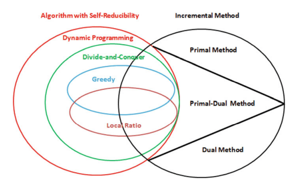
计算机代写|组合优化代写Combinatorial optimization代考|Algorithms with Self-Reducibility
There exist a large number of algorithms in which the problem is reduced to several subproblems, each of which is the same problem on a smaller-size input. Such a problem is said to have the self-reducibility, and the algorithm is said to be with self-reducibility.
For example, consider sorting problem again. Suppose input contains $n$ numbers. We may divide these $n$ numbers into two subproblems. One subproblem is the sorting problem on $\lfloor n / 2\rfloor$ numbers, and the other subproblem is the sorting problem on $\lceil n / 2\rceil$ numbers. After completely sorting each subproblem, combine two sorted sequences into one. This idea will result in a sorting algorithm, called the merge sort. The pseudocode of this algorithm is shown in Algorithm 1.
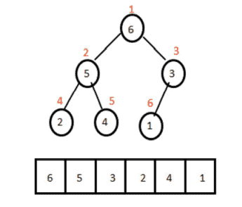
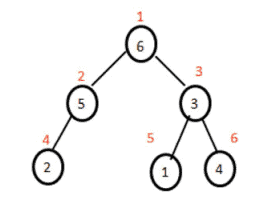
The main body calls a procedure. This procedure contains two self-calls, which means that the merge sort is a recursive algorithm, that is, the divide will continue until each subproblem has input of single number. Then this procedure employs another procedure (Merge) to combine solutions of subproblems with smaller inputs into subproblems with larger inputs. This computation process on input ${5,2,7,4,6,8,1,3}$ is shown in Fig. 2.1.
Note that the running time of procedure Merge at each level is $O(n)$. Let $t(n)$ be the running time of merge sort on input of size $n$. By the recursive structure, we can obtain that $t(1)=0$ and $$ t(n)=t(\lfloor n / 2\rfloor)+t(\lceil n / 2\rceil)+O(n) . $$ Suppose $$ t(n) \leq 2 \cdot t([n / 2\rceil)+c \cdot n $$ for some positive constant $c$. Define $T(1)=0$ and $$ T(n)=2 \cdot T(\lceil n / 2\rceil)+c \cdot n . $$ By induction, we can prove that $$ t(n) \leq T(n) \text { for all } n \geq 1 . $$
计算机代写|组合优化代写Combinatorial optimization代考|Optimal and Approximation Solutions
Let us show an optimality condition for the minimum spanning tree. Theorem 1.2.1 (Path Optimality) A spanning tree $T^*$ is a minimum spanning tree if and only if it satisfies the following condition:
Path Optimality Condition For every edge $(u, v)$ not in $T^$, there exists a path $p$ in $T^$, connecting $u$ and $v$, and moreover, $c(u, v) \geq c(x, y)$ for every edge $(x, y)$ in path $p$.
Proof Suppose, for contradiction, that $c(u, v)<c(x, y)$ for some edge $(x, y)$ in the path $p$. Then $T^{\prime}=\left(T^* \backslash(x, y)\right) \cup(u, v)$ is a spanning tree with cost less than $c\left(T^\right)$, contradicting the minimaality of $T^$.
Conversely, suppose that $T^$ satisfies the path optimality condition. Let $T^{\prime}$ be a minimum spanning tree such that among all minimum spanning tree, $T^{\prime}$ is the one with the most edges in common with $T^$. Suppose, for contradiction, that $T^{\prime} \neq T^$. We claim that there exists an edge $(u, v) \in T^$ such that the path in $T^{\prime}$ between $u$ and $v$ contains an edge $(x, y)$ with length $c(x, y) \geq c(u, v)$. If this claim is true, then $\left(T^{\prime} \backslash(x, y)\right) \cup(u, v)$ is still a minimum spanning tree, contradicting the definition of $T^{\prime}$.
Now, we show the claim by contradiction. Suppose the claim is not true. Consider an edge $\left(u_1, v_1\right) \in T^* \backslash T^{\prime}$. the path in $T^{\prime}$ connecting $u_1$ and $v_1$ must contain an edge $\left(x_1, y_1\right)$ not in $T^$. Since the claim is not true, we have $c\left(u_1, v_1\right)$ connecting $x_1$ and $y_1$, which must contain an edge $\left(u_2, v_2\right) \notin$ $T^{\prime}$. Since $T^$ satisfies the path optimality condition, we have $c\left(x_1, y_1\right) \leq c\left(u_2, v_2\right)$. Hence, $c\left(u_1, v_1\right)$ such that $c\left(u_1, v_2\right)<c\left(u_2, v_2\right)<c\left(u_3, v_3\right)<\cdots$, contradicting the finiteness of $T^*$.
计算机代写|组合优化代写Combinatorial optimization代考|Running Time
The most important measure of quality for algorithms is the running time. However, for the same algorithm, it may take different times when we run it in different computers. To give a uniform standard, we have to get an agreement that runs algorithms in a theoretical computer model. This model is the multi-tape Turing machine which has been accepted by a very large population. Based on the Turing machine, the theory of computational complexity has been built up. We will touch this part of theory in Chap. 8 .
But, we will use RAM model to evaluate the running time for algorithms throughout this book except Chap. 8. In RAM model, assume that each line of pseudocode requires a constant time. For example, the running time of insertion sort is calculated in Fig. 1.6.
Actually, RAM model and Turing machine model are closely related. The running time estimated based on these two models is considered to be close enough. However, they are sometimes different in estimation of running time. For example, the following is a piece of pseudocode. $$ f(n) \leq c \cdot g(n) \text { for } n \geq n_0 $$
There are two more notations which appear very often in representation of running time. $f(n)=\Omega 2(g(n))$ means that there exist constant $c>0$ and $n_0>0$ such that $0 \leq c \cdot g(n) \leq f(n)$ for $n \geq n_0$. $f(n)=\Theta(g(n))$ means that there exist constants $c_1>0, c_2>0$ and $n_0>0$ such that $$ c_1 \cdot g(n) \leq f(n) \leq c_2 \cdot g(n) \text { for } n \geq n_0 . $$ Finally, let us make a remark on input numbers. In the minimum spanning tree problem, every edge has a nonnegative weight which is an input number. In the problem definition, we assumed that this is a real number. However, a real number cannot be exactly input in a computer. Actually, the computation of a real number is sometimes a very hard problem in the theory of computational complexity [260]. Therefore, we have to treat each real number with an oracle which can provide a rational number with expected accuracy, without computation cost. In other words, we ignore the computation trouble of the real number.
However, when our analysis of running time has to consider the size of input numbers, e.g., in analysis of weakly polynomial-time algorithms, we have to change the setting from the real number to the integer.
数学代写|组合优化代写Combinatorial optimization代考|Eulerian and Bipartite Graphs
Euler’s work on the problem of traversing each of the seven bridges of Königsberg exactly once was the origin of graph theory. He showed that the problem had no solution by defining a graph, asking for a walk containing all edges, and observing that more than two vertices had odd degree.
Definition 2.23. An Eulerian walk in a graph $G$ is a closed walk containing every edge. An undirected graph $G$ is called Eulerian if the degree of each vertex is even. A digraph $G$ is Eulerian if $\left|\delta^{-}(v)\right|=\left|\delta^{+}(v)\right|$ for each $v \in V(G)$.
Although Euler neither proved sufficiency nor considered the case explicitly in which we ask for a closed walk, the following famous result is usually attributed to him:
Theorem 2.24. (Euler [1736], Hierholzer [1873]) A connected (directed or undirected) graph has an Eulerian walk if and only if it is Eulerian.
Proof: The necessity of the degree conditions is obvious, as a vertex appearing $k$ times in an Eulerian walk (or $k+1$ times if it is the first and the last vertex) must have in-degree $k$ and out-degree $k$, or degree $2 k$ in the undirected case.
For the sufficiency, let $W=v_1, e_1, v_2, \ldots, v_k, e_k, v_{k+1}$ be a longest walk in $G$, i.e. one with maximum number of edges. In particular, $W$ must contain all edges leaving $v_{k+1}$, which implies $v_{k+1}=v_1$ by the degree conditions. So $W$ is closed. Suppose that $W$ does not contain all edges. As $G$ is connected, we then conclude that there is an edge $e \in E(G)$ for which $e$ does not appear in $W$, but at least one of its endpoints appears in $W$, say $v_i$. Then $e$ can be combined with $v_i, e_i, v_{i+1}, \ldots, e_k, v_{k+1}=v_1, e_1, v_2, \ldots, e_{i-1}, v_i$ to a walk which is longer than $W$.
We shall now introduce an important duality concept. In this section, graphs may contain loops, i.e. edges whose endpoints coincide. In a planar embedding loops are of course represented by polygons instead of polygonal arcs.
Note that Euler’s formula (Theorem 2.32) also holds for graphs with loops: this follows from the observation that subdividing a loop $e$ (i.e. replacing $e={v, v}$ by two parallel edges ${v, w},{w, v}$ where $w$ is a new vertex) and adjusting the embedding (replacing the polygon $J_e$ by two polygonal arcs whose union is $J_e$ ) increases the number of edges and vertices each by one but does not change the number of faces.
Definition 2.41. Let $G$ be a directed or undirected graph, possibly with loops, and let $\Phi=\left(\psi,\left(J_e\right){e \in E(G)}\right)$ be a planar embedding of $G$. We define the planar dual $G^$ whose vertices are the faces of $\Phi$ and whose edge set is $\left{e^: e \in E(G)\right}$, where $e^$ connects the faces that are adjacent to $J_e$ (if $J_e$ is adjacent to only one face, then $e^$ is a loop). In the directed case, say for $e=(v, w)$, we orient $e^=\left(F_1, F_2\right)$ in such a way that $F_1$ is the face “to the right” when traversing $J_e$ from $\psi(v)$ to $\psi(w)$. $G^$ is again planar. In fact, there obviously exists a planar embedding $\left(\psi^,\left(J{e^}\right)_{e^* \in E\left(G^\right)}\right)$ of $G^$ such that $\psi^*(F) \in F$ for all faces $F$ of $\Phi$ and, for each $e \in E(G)$,
$$ J_{e^} \cap\left({\psi(v): v \in V(G)} \cup \bigcup_{f \in E(G) \backslash{e}} J_f\right)=\emptyset, $$ $\left|J_{e^} \cap J_e\right|-1$, and if $e^$ is a loop then the face bounded by $J_{e^}$ contains exactly one endpoint of $e$. Such an embedding is called a standard embedding of $G^*$.
数学代写|组合优化代写Combinatorial optimization代考|Trees, Circuits, and Cuts
An undirected graph $G$ is called connected if there is a $v$-w-path for all $v, w \in$ $V(G)$; otherwise $G$ is disconnected. A digraph is called connected if the underlying undirected graph is connected. The maximal connected subgraphs of a graph are its connected components. Sometimes we identify the connected components with the vertex sets inducing them. A set of vertices $X$ is called connected if the subgraph induced by $X$ is connected. A vertex $v$ with the property that $G-v$ has more connected components than $G$ is called an articulation vertex. An edge $e$ is called a bridge if $G-e$ has more connected components than $G$.
An undirected graph without a circuit (as a subgraph) is called a forest. A connected forest is a tree. A vertex of degree at most 1 in a tree is called a leaf. A star is a tree where at most one vertex is not a leaf.
In the following we shall give some equivalent characterizations of trees and their directed counterparts, arborescences. We need the following connectivity criterion: Proposition 2.3. (a) An undirected graph $G$ is connected if and only if $\delta(X) \neq \emptyset$ for all $\emptyset \neq X \subset$ $V(G)$ (b) Let $G$ be a digraph and $r \in V(G)$. Then there exists an $r$-v-path for every $v \in V(G)$ if and only if $\delta^{+}(X) \neq \emptyset$ for all $X \subset V(G)$ with $r \in X$.
Proof: (a): If there is a set $X \subset V(G)$ with $r \in X, v \in V(G) \backslash X$, and $\delta(X)=$ $\emptyset$, there can he no $r-11$-path, so $G$ is not connected. On the other hand, if $G$ is not connected, there is no $r-v$-path for some $r$ and $v$. Let $R$ be the set of vertices reachable from $r$. We have $r \in R, v \notin R$ and $\delta(R)=\emptyset$. (b) is proved analogously.
The incidence matrix of a digraph $G$ is the matrix $A=\left(a_{v, e}\right){v \in V(G), e \in E(G)}$ where $$ a{v,(x, y)}=\left{\begin{array}{ll} -1 & \text { if } v=x \ 1 & \text { if } v=y \ 0 & \text { if } v \notin{x, y} \end{array} .\right. $$ Of course this is not very efficient since each column contains only two nonzero entries. The space needed for storing an incidence matrix is obviously $O(\mathrm{~nm})$, where $n:=|V(G)|$ and $m:=|E(G)|$.
A better way is a matrix whose rows and columns are indexed by the vertex set. The adjacency matrix of a simple graph $G$ is the 0-1-matrix $A=\left(a_{v, w}\right){v, w \in V(G)}$ with $a{v, w}=1$ iff ${v, w} \in E(G)$ or $(v, w) \in E(G)$. For graphs with parallel edges we can define $a_{v, w}$ to be the number of edges from $v$ to $w$. An adjacency matrix requires $O\left(n^2\right)$ space for simple graphs.
The adjacency matrix is appropriate if the graph is dense, i.e. has $\Theta\left(n^2\right)$ edges (or more). For sparse graphs, say with $O(n)$ edges only, one can do much better. Besides storing the number of vertices we can simply store a list of the edges, for each edge noting its endpoints. If we address each vertex by a number from 1 to $n$, the space needed for each edge is $O(\log n)$. Hence we need $O(m \log n)$ space altogether.
Just storing the edges in an arbitrary order is not very convenient. Almost all graph algorithms require finding the edges incident to a given vertex. Thus one should have a list of incident edges for each vertex. In case of directed graphs, two lists, one for entering edges and one for leaving edges, are appropriate. This data structure is called adjacency list; it is the most customary one for graphs. For direct access to the list(s) of each vertex we have pointers to the heads of all lists; these can be stored with $O(n \log m)$ additional bits. Hence the total number of bits required for an adjacency list is $O(n \log m+m \log n)$.
Whenever a graph is part of the input of an algorithm in this book, we assume that the graph is given by an adjacency list.
As for elementary operations on numbers (see Section 1.2), we assume that elementary operations on vertices and edges take constant time only.
如果所有$v, w \in$$V(G)$都有$v$ -w-path,则无向图$G$称为connected;否则$G$将断开连接。如果底层的无向图是连通的,则有向图称为连通的。图的最大连通子图是它的连通分量。有时我们用顶点集来确定连接的分量。如果由$X$诱导的子图是连通的,则称之为连通的顶点集$X$。顶点$v$具有$G-v$比$G$具有更多连接组件的属性,称为连接顶点。如果$G-e$比$G$连接的组件更多,则边$e$被称为桥接
Now, we give the main result of the paper which is a new family of valid inequalities for the BBFLP. These latter inequalities are obtained by lifting the rounded cut-set inequalities.
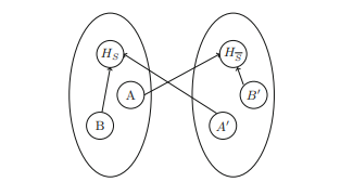
Consider the situation where all the facilities are opened and all the clients are assigned to a facility. For every $j \in D$, let $h_{j}$ be the facility to which it is assigned (Fig. 1). Let $Q_{0}=\left{(x, y, t) \in Q\right.$ such that $t_{j}^{h}=0$, for all $\left.h \in H \backslash h_{j}, j \in D\right}$. Lemma 1. The solutions of $Q_{0}$ are exactly solutions of a NLP where the demand set is composed of the pairs $\left(j, h_{j}\right)$, with $j$ the origin, $h_{j}$ the destination and $d_{j}$ is the commodity.
By Lemma 1, every valid inequality (respectively facet defining) for the corresponding NLP polyhedron are valid for $Q_{0}$ (respectively facet defining). This means that rounded cut-set inequalities are valid for $Q_{0}$.
Our objective is to extend the rounded cut-set inequalities by a lifting procedure to obtain facet defining inequalities for BBFLP. Let $(x, y, t) \in Q_{0}$ and $S \subseteq V$ be a node set such that $S \cap V \neq \emptyset \neq \bar{S} \cap V$. Let $A$ (resp. $A^{\prime}$ ) be the node subset of $D \cap S$ (resp. $D \cap \bar{S}$ ) which are assigned to a facility of $H \cap \bar{S}$ (resp. $H \cap S$ ). Also, let $B$ (resp. $B^{\prime}$ ) be the node subset of $D \cap S$ (resp. $D \cap \bar{S}$ ) which are assigned to a facility of $H \cap S$ (resp. $H \cap \bar{S}$ ). The rounded cut-set inequality induced by $S$ is $$ x^{1}(\delta(S))+r x^{2}(\delta(S)) \geq r\left\lceil\frac{d\left(A \cup A^{\prime}\right)}{C}\right\rceil, $$ where $r=d\left(A \cup A^{\prime}\right)(\bmod C)$. Clearly (24) is valid for $Q_{0}$. For convenience, we let, $$ \begin{aligned} &A_{1}=\left{j \in A \cup A^{\prime} \text { such that } d_{j} \leq r\right} \ &A_{2}=\left{j \in A \cup A^{\prime} \text { such that } d_{j}>r\right} \ &B_{1}=\left{j \in B \cup B^{\prime} \text { such that } d_{j} \leq C-r\right}, \ &B_{2}=\left{j \in B \cup B^{\prime} \text { such that } d_{j}>C-r\right} . \end{aligned} $$ Now we give our main result. Theorem 4. Let $S \subseteq V$ with $S \cap V \neq \emptyset \neq V \cap \bar{S}$. The inequality $$ x^{1}(\delta(S))+r x^{2}(\delta(S))+\sum_{j \in D} \sum_{\left.h \in H \backslash h_{j}\right}} C_{j}^{h} t_{j}^{h} \geq r\left\lceil\frac{d\left(A \cup A^{\prime}\right)}{C}\right\rceil $$ where $$ C_{j}^{h}=\left{\begin{array}{l} d_{j}, \text { for } j \in A_{1} \cap A, h \in H \cap S \text { and for } \in A_{1} \cap A^{\prime}, h \in H \cap \bar{S}, \ r, \text { for } j \in A_{2} \cap A, h \in H \cap S \text { and for } j \in A_{2} \cap A^{\prime}, h \in H \cap \bar{S} \ C-r-d_{j}, \text { for } j \in B_{1} \cap B, h \in H \cap \bar{S} \text { and for } j \in B_{1} \cap B^{\prime}, h \in H \cap S, \ 0, \text { otherwise. } \end{array}\right. $$ is valid for BBFLP. Moreover (25) is facet for $Q$ if (24) is facet for $Q_{0}$.
We now consider our second example given initially, the JOB ASSIGNMENT PROBLEM, and briefly address some central topics which will be discussed in later chapters.
The Job Assignment Problem is quite different to the DRILLING PROBLEM since there are infinitely many feasible solutions for each instance (except for trivial cases). We can reformulate the problem by introducing a variable $T$ for the time when all jobs are done: $$ \min T $$ $\begin{aligned} \text { s.t. } \quad \sum_{j \in S_i} x_{i j} &=t_i & &(i \in{1, \ldots, n}) \ x_{i j} & \geq 0 & &\left(i \in{1, \ldots, n}, j \in S_i\right) \ \sum_{i: j \in S_i} x_{i j} \leq T & &(j \in{1, \ldots, m}) \end{aligned}$ The numbers $t_i$ and the sets $S_i(i=1, \ldots, n)$ are given, the variables $x_{i j}$ and $T$ are what we look for. Such an optimization problem with a linear objective function and linear constraints is called a linear program. The set of feasible solutions of (1.1), a so-called polyhedron, is easily seen to be convex, and one can prove that there always exists an optimum solution which is one of the finitely many extreme points of this set. Therefore a linear program can, theoretically, also be solved by complete enumeration. But there are much better ways as we shall see later.
Although there are several algorithms for solving linear programs in general, such general techniques are usually less efficient than special algorithms exploiting the structure of the problem. In our case it is convenient to model the sets $S_i, i=$ $1, \ldots, n$, by a graph. For each job $i$ and for each employee $j$ we have a point (called vertex), and we connect employee $j$ with job $i$ by an edge if he or she can contribute to this job (i.e. if $j \in S_i$ ). Graphs are a fundamental combinatorial structure; many combinatorial optimization problems are described most naturally in terms of graph theory.
Suppose for a moment that the processing time of each job is one hour, and we ask whether we can finish all jobs within one hour. So we look for numbers $x_{i j}$ $\left(i \in{1, \ldots, n}, j \in S_i\right)$ such that $0 \leq x_{i j} \leq 1$ for all $i$ and $j, \sum_{j \in S_i} x_{i j}=1$ for $i=1, \ldots, n$, and $\sum_{i: j \in S_i} x_{i j} \leq 1$ for $j=1, \ldots, n$. One can show that if such a solution exists, then in fact an integral solution exists, i.e. all $x_{i j}$ are either 0 or 1 . This is equivalent to assigning each job to one employee, such that no employee has to do more than one job. In the language of graph theory we then look for a matching covering all jobs. The problem of finding optimal matchings is one of the best-known combinatorial optimization problems.
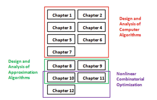
We review the basics of graph theory and linear programming in Chapters 2 and 3. In Chapter 4 we prove that linear programs can be solved in polynomial time, and in Chapter 5 we discuss integral polyhedra. In the subsequent chapters we discuss some classical combinatorial optimization problems in detail.
数学代写|组合优化代写Combinatorial optimization代考|Network Loading and Valid Inequalities
Several families of valid inequalities were introduced for the problem, in the following we will give the basic valid inequalities that define facets. The NLP with two cables types is formulated as follows. Let $G=(V, E)$ be an undirected graph, a set of $M$ commodities $\left{\left(s_{1}, t_{1}\right), \ldots,\left(s_{|M|}, t_{|M|}\right)\right}$, a commodity $q \in{1, \ldots, M}$ having a demand $d_{q}$. $$ \begin{aligned} &\min \sum_{u \in E E} l_{u v} \gamma^{1} x_{u E}^{1}+l_{w v} \gamma^{2} x_{u E}^{2} \ &\sum_{v \in V} f_{(u, v)}^{q}-\sum_{v \in V} f_{(v, w)}^{q}=\left{\begin{array}{ll} d_{q}, \text { if } u=s_{q} \ -d_{q}, \text { if } u=t_{q}, \ 0, & \text { otherwise. } \end{array} \quad \text { for all } u \in V, q \in{1, \ldots, M}(17)\right. \end{aligned} $$ $$ \begin{aligned} &\sum_{q=1}^{M}\left(f_{(u, v)}^{k}+f_{(v, u)}^{k}\right) \leq x_{u v}^{1}+C x_{u v}^{2} \ &x_{e}^{1}, x_{e}^{2} \geq 0, \quad \text { for all } e \in E, \ &f_{(u, v)}^{k}, f_{(v, u)}^{k} \geq 0 \text { for all } u v \in E, k \in K . \end{aligned} $$ Rounded Cut-Set Inequalities. The rounded cut-set inequalities are obtained by partitioning the node set into two subsets, namely $S$ and $\bar{S}$. Magnanti et al. [14] introduced the following form for the rounded cut-set inequalities: $$ x^{1}(\delta(S))+r x^{2}(\delta(S)) \geq r\left\lceil\frac{D_{S, \bar{S}}}{C}\right\rceil $$
where $D_{S, \bar{S}}$ is the total demand whose origin lays in $S$ and destination in $\bar{S}$ and vice-versa, and $$ r=\left{\begin{array}{l} C, \text { if } \quad D_{S, \bar{S}} \quad(\bmod C)=0 \ D_{S, \bar{S}} \quad(\bmod C), \text { otherwise. } \end{array}\right. $$ Theorem 3 [14]. A rounded cut set inequality defines a facet for the $N L P$ if and only if
the subgraphs induced by $S$ and by $\bar{S}$ are connected,
$D_{S, \bar{S}}>0$. Partition Inequalities. Several version of partition inequalities have been developed in the literature, in particular, Magnanti et al. [14] gave a family of three-partition inequalities of the following form: $$ x_{12}^{1}+x_{13}^{1}+x_{23}^{1}+r\left(x_{12}^{2}+x_{13}^{2}+x_{23}^{2}\right) \geq\left\lceil\left[\frac{r\left(\left\lceil\frac{d_{12}+d_{13}}{C}\right\rceil+\left\lceil\frac{d_{12}+d_{23}}{C}\right\rceil+\left\lceil\frac{d_{13}+d_{23}}{C}\right\rceil\right)}{2}\right\rceil\right. $$ The following metric inequalities are valid for NLP with one cable type: Metric Inequalities. Metric inequalities can be introduced after projecting out the flow variables from the polyhedron and obtain a “capacity formulation” in the space of capacity variables. In particular Avella et al. [2] gave a family of metric inequalities that completely describe the polyhedron, they take the form $$ \mu x \geq \rho(\mu, G, d), \mu \in \operatorname{Met}(G) $$ In the next section we present a lifting procedure that extends the Rounded cut-set inequalities defined for NLP to be valid for BBFLP.
Now, we give the main result of the paper which is a new family of valid inequalities for the BBFLP. These latter inequalities are obtained by lifting the rounded cut-set inequalities.
Consider the situation where all the facilities are opened and all the clients are assigned to a facility. For every $j \in D$, let $h_{j}$ be the facility to which it is assigned (Fig. 1). Let $Q_{0}=\left{(x, y, t) \in Q\right.$ such that $t_{j}^{h}=0$, for all $\left.h \in H \backslash h_{j}, j \in D\right}$. Lemma 1. The solutions of $Q_{0}$ are exactly solutions of a NLP where the demand set is composed of the pairs $\left(j, h_{j}\right)$, with $j$ the origin, $h_{j}$ the destination and $d_{j}$ is the commodity.
By Lemma 1, every valid inequality (respectively facet defining) for the corresponding NLP polyhedron are valid for $Q_{0}$ (respectively facet defining). This means that rounded cut-set inequalities are valid for $Q_{0}$.
Our objective is to extend the rounded cut-set inequalities by a lifting procedure to obtain facet defining inequalities for BBFLP. Let $(x, y, t) \in Q_{0}$ and $S \subseteq V$ be a node set such that $S \cap V \neq \emptyset \neq \bar{S} \cap V$. Let $A$ (resp. $A^{\prime}$ ) be the node subset of $D \cap S$ (resp. $D \cap \bar{S}$ ) which are assigned to a facility of $H \cap \bar{S}$ (resp. $H \cap S$ ). Also, let $B$ (resp. $B^{\prime}$ ) be the node subset of $D \cap S$ (resp. $D \cap \bar{S}$ ) which are assigned to a facility of $H \cap S$ (resp. $H \cap \bar{S}$ ). The rounded cut-set inequality induced by $S$ is $$ x^{1}(\delta(S))+r x^{2}(\delta(S)) \geq r\left\lceil\frac{d\left(A \cup A^{\prime}\right)}{C}\right\rceil, $$ where $r=d\left(A \cup A^{\prime}\right)(\bmod C)$. Clearly (24) is valid for $Q_{0}$. For convenience, we let, $$ \begin{aligned} &A_{1}=\left{j \in A \cup A^{\prime} \text { such that } d_{j} \leq r\right} \ &A_{2}=\left{j \in A \cup A^{\prime} \text { such that } d_{j}>r\right} \ &B_{1}=\left{j \in B \cup B^{\prime} \text { such that } d_{j} \leq C-r\right}, \ &B_{2}=\left{j \in B \cup B^{\prime} \text { such that } d_{j}>C-r\right} . \end{aligned} $$ Now we give our main result. Theorem 4. Let $S \subseteq V$ with $S \cap V \neq \emptyset \neq V \cap \bar{S}$. The inequality $$ x^{1}(\delta(S))+r x^{2}(\delta(S))+\sum_{j \in D} \sum_{\left.h \in H \backslash h_{j}\right}} C_{j}^{h} t_{j}^{h} \geq r\left\lceil\frac{d\left(A \cup A^{\prime}\right)}{C}\right\rceil $$ where $$ C_{j}^{h}=\left{\begin{array}{l} d_{j}, \text { for } j \in A_{1} \cap A, h \in H \cap S \text { and for } \in A_{1} \cap A^{\prime}, h \in H \cap \bar{S}, \ r, \text { for } j \in A_{2} \cap A, h \in H \cap S \text { and for } j \in A_{2} \cap A^{\prime}, h \in H \cap \bar{S} \ C-r-d_{j}, \text { for } j \in B_{1} \cap B, h \in H \cap \bar{S} \text { and for } j \in B_{1} \cap B^{\prime}, h \in H \cap S, \ 0, \text { otherwise. } \end{array}\right. $$ is valid for BBFLP. Moreover (25) is facet for $Q$ if (24) is facet for $Q_{0}$.
数学代写|组合优化代写Combinatorial optimization代考|A Polyhedral Study for the Buy-at-Bulk Facility Location Problem
Lemma 3. If $D^{\prime}=\emptyset$ then, for every $j_{0} \in A \cup A^{\prime}$ and $h_{0} \in H \backslash\left{h_{j_{0}}\right}$, $$ \xi_{j_{0}}^{h_{0}}=r\left\lceil\frac{d(W)}{C}\right\rceil+\varepsilon_{W} $$ where $W=\left(A \cup A^{\prime}\right) \backslash\left{j_{0}\right}$. Proof. First, let $\beta$ be the number of cables of type 1 loaded on the edges of $\delta(S)$. Also, w.l.o.g., we assume that the number of cables of type 2 loaded on the edges of $\delta(S)$ is $\left\lceil\frac{d(W)}{C}\right\rceil-\lambda$, for some $\lambda \geq 0$. In any feasible solution of the BBFLP, we have that $\beta+C\left(\left\lceil\frac{d(W)}{C}\right\rceil-\lambda\right) \geq d(W)$.
We have that $x^{1}(\delta(S))+r x^{2}(\delta(S))=\beta+r\left(\left\lceil\frac{d(W)}{C}\right\rceil-\lambda\right)$. If $\lambda=0$, we can show that the minimum value of $x^{1}(\delta(S))+r x^{2}(\delta(S))$ is obtained for $\beta=0$. Thus, $\xi_{j_{0}}^{h_{0}}=r\left\lceil\frac{d(W)}{C}\right\rceil$ in this case. Now, if $\lambda \geq 1$, we have that $$ \beta+r\left(\left\lceil\frac{d(W)}{C}\right\rceil-\lambda\right) \geq(C-r) \lambda-C+r_{W}+r\left\lceil\frac{d(W)}{C}\right\rceil . $$ Here also, we can show that the minimum of $x^{1}(\delta(S))+r x^{2}(\delta(S))$ is obtained for $\lambda=1$ and $\beta=C(\lambda-1)+r_{W}=r_{W}$, that is $\xi_{j_{0}}^{h_{0}}=r_{W}-r+r\left\lceil\frac{d(W)}{C}\right\rceil$. Thus, $\xi_{j_{0}}^{h_{0}}=r\left\lceil\frac{d(W)}{C}\right\rceil+\min \left{0, r_{W}-r\right}=r\left\lceil\frac{d(W)}{C}\right\rceil+\varepsilon_{W}$. Lemma 4. If $D^{\prime}=\emptyset$ then, for every $j_{0} \in B \cup B^{\prime}$ and $h_{0} \in H \backslash\left{h_{j_{0}}\right}$, $$ \xi_{j_{0}}^{h_{0}}=r\left\lceil\left[\frac{d(W)}{C}\right\rceil+\varepsilon_{W}\right. $$ where $W=A \cup A^{\prime} \cup\left{j_{0}\right}$. Now, for a node set $U \subseteq D$, we let $$ \alpha_{U}=\left\lceil\frac{d\left(A \cup A^{\prime}\right)}{C}\right\rceil-\left\lceil\frac{d(U)}{C}\right\rceil . $$ From Lemmas 3 and 4 , when $D^{\prime}=\emptyset$, the lifting coefficient of a variable $t_{j_{0}}^{h_{0}}$ is of the form $$ C_{j_{0}}^{h_{0}}=r \alpha_{W}-\varepsilon_{W} $$ where $$ W=\left{\begin{array}{l} \left(A \cup A^{\prime}\right) \backslash\left{j_{0}\right}, \text { for } j_{0} \in A \cup A^{\prime}, \ A \cup A^{\prime} \cup\left{j_{0}\right}, \text { for } j_{0} \in B \cup B^{\prime} . \end{array}\right. $$ From this, we can see that the lifting coefficient of variable $t_{j}^{h}$, when $D^{\prime}=\emptyset$ ({i.e. $}$ when the variable is lifted at first), is $-C_{j}^{h}=r \alpha_{W}-\varepsilon_{W}=d_{j}$, for $j \in A_{1}$, $-C_{j}^{h}=r \alpha_{W}-\varepsilon_{W}=r$, for $j \in A_{2}$, $-C_{j}^{h}=r \alpha_{W}-\varepsilon_{W}=0$, for $j \in B_{1}$, $-C_{j}^{h}=r \alpha_{W}-\varepsilon_{W}=C-r-d_{j}$, for $j \in B_{2} .$
数学代写|组合优化代写Combinatorial optimization代考|Network Loading and Valid Inequalities
为这个问题引入了几个有效不等式族,下面我们将给出定义方面的基本有效不等式。 具有两种电缆类型的 NLP 公式如下。 让G=(V,E)是一个无向图,一组M商品\left{\left(s_{1}, t_{1}\right), \ldots,\left(s_{|M|}, t_{|M|}\right)\right}\left{\left(s_{1}, t_{1}\right), \ldots,\left(s_{|M|}, t_{|M|}\right)\right}, 一种商品q∈1,…,M有需求dq. $$ \begin{aligned} &\min \sum_{u \in EE} l_{uv} \gamma^{1} x_{u E}^{1}+l_{wv} \gamma^{2} x_{ u E}^{2} \ &\sum_{v \in V} f_{(u, v)}^{q}-\sum_{v \in V} f_{(v, w)}^{q} =\左{dq, if u=sq −dq, if u=tq, 0, otherwise. \quad \text { for all } u \in V, q \in{1, \ldots, M}(17)\right. \end{对齐}
∑q=1M(f(u,v)k+f(v,u)k)≤xuv1+Cxuv2 xe1,xe2≥0, for all e∈E, f(u,v)k,f(v,u)k≥0 for all uv∈E,k∈K. RoundedCut−SetInequalities.Theroundedcut−setinequalitiesareobtainedbypartitioningthenodesetintotwosubsets,namely$S$and$S¯$.Magnantietal.[14]introducedthefollowingformfortheroundedcut−setinequalities: x^{1}(\delta(S))+rx^{2}(\delta(S)) \geq r\left\lceil\frac{D_{S, \bar{S}}}{C}\对\rceil $$
The Buy-at-Bulk facility location problem (BBFLP for short) is defined by an undirected graph $G=(V, E)$, where $V$ denotes the set of nodes and $E$ denotes the set of edges. We are given a set of clients $D \subseteq V$ and a set of facilities $H \subseteq V$. Each client $j \in D$ has a positive demand $d_{j}$. Each facility $h \in H$ is associated with an opening cost $\mu_{h}$. We also have a set $K$ of different cable types. Each cable type $k \in K$ has a capacity $u_{k}$ and a set-up cost per unit length denoted by $\gamma_{k}$. Finally, for each edge $e \in E$ we consider a length $l_{e} \in \mathbb{Z}^{+}$. We assume that the cable types satisfy the so-called economies of scales in that if we let $K={1, \ldots,|K|}$ such that $u_{1} \leq u_{2} \leq \ldots \leq u_{K}, \gamma_{1} \leq \gamma_{2} \leq \ldots \leq \gamma_{K}$, and $\gamma_{1} / u_{1} \geq \gamma_{2} / u_{2} \geq \ldots \geq \gamma_{K} / u_{K}$. A solution of the BBFLP consists in choosing
a set of facilities to open.
an assignment of each client to exactly one opened facility,
a number of cables of each type to be installed on each edge of the graph in order to route the demands from each client to the facility to which it is assigned.
The BBFLP is closely related to the facility location problem and network loading problem. It has many applications in telecommunications and transportation network design. It is not hard to see that the BBFLP contains the Facility Location problem and hence it is NP-hard.
In the literature, the BBFLP was mainly studied in the perspective of approximation algorithms. It was first studied by Meyrson et al. [17] who considered a cost-distance problem and present the BBFLP as a special case of this latter problem. In their work, they provided an $O(\log |D|)$ approximation algorithm. Ravi et al. [19] gave an $O(k)$ approximation algorithm for the BBFLP where $k$ is the number of cable types. Later, Friggst et al. [13] considered an integer programming formulation for the BBFLP, and showed that this formulation has an integrality gap of $O(k)$. They also considered the variant of the BBFLP where the opened facilities must be connected and gave an integrality gap of $O(1)$. Recently, Bley et al. [7] presented the first exact algorithm for the problem. They introduced a path-based formulation for the problem and compare it with a compact flow-based formulation. They also design an exact branch-and-priceand-cut algorithm for solving the path-based formulation.
As mentioned before, the BBFLP is related to the Network Loading Problem (NLP) and the Facility Location Problem (FLP). Both problems have received a lot of attention. Concerning, the NLP, Magnanti et al. [14] studied the NLP from a polyhedral point of view. They introduced some classes of valid inequalities and devised a Branch-and-Cut algorithm. In [15], Magnanti et al. considered the NLP with two cable types and some particular graphs and gave a complete description of the associated polyhedron in these cases. Bienstock et al. [6] studied the NLP with two cable types with possible extension to more than three cable types. Barahona [9] addressed the same problem, he used a relaxation without flow variables, this relaxation is based on cut condition for multicommodity flows. Gülnük [11] gave a branch and cut algorithm using spanning tree inequalities and mixed integer rounding inequalities. Agarwal [3] has introduced 4-partition based facets. Agarwal [4] extended his previous work and get a complete description of the 4-node network design problem. Raacker et al. [18] have extended the polyhedral results for cut-based inequalities for network design problem with directed, bidirected and undirected link-capacity models. Agarwal [5] developed the total-capacity inequalities, one-two inequalities and spanning trees inequalities based on a p-partition of the graph and discuss conditions under which these inequalities are facet-defining.
数学代写|组合优化代写Combinatorial optimization代考|Integer Programming Formulation and Polyhedron
Now, we give the so-called cut formulation for the BBFLP. This formulation can be obtained by slightly modifying the flow-based formulation introduced by [7] and projecting out the flow variables. The cut formulation is given below. Variable $t_{j}^{h}$ equals 1 if the client $j$ is assigned to facility $h$, for all $j \in D$ and $h \in H$, and $x_{e}^{k}$ is the number of cable of type $k$ installed on edge $e$, for all $e \in E$ and $k \in K$. $\min \sum_{h \in H} \mu_{h} y_{h}+\sum_{e \in E} \sum_{k \in K} \gamma^{k} l_{e}^{k} x_{e}^{k}$ $\sum_{h \in H} t_{j}^{h}=1$, for all $j \in D$ $t_{j}^{h} \leq y_{h}$, for all $h \in H, j \in D$ $h \in H, j \in D$ $\sum_{\varepsilon \in \delta(W)} \sum_{k \in K} u_{k} x_{e}^{k} \geq \sum_{j \in W \cap D_{h}} \sum_{h \cap H \bar{S}} t_{j}^{h} d_{j}+\sum_{j \in W \cap D} \sum_{h \in H \cap S} t_{j}^{h} d_{j}$, for all $W \subseteq D$, $S \subseteq V, \bar{S} \subseteq V \backslash S \quad$ (3) $t_{j}^{h} \geq 0, \quad$ for all $h \in H, j \in D$, (4) $y_{h} \leq 1, \quad$ for all $h \in H$, $x_{e}^{k} \geq 0, \quad$ for all $k \in K, e \in E$, (6) $t_{j}^{h} \in{0,1}, \quad$ for all $h \in H, j \in D$, (7) $y_{h} \in{0,1}, \quad$ for all $h \in H$, $x_{e}^{k} \in \mathbb{Z}^{+}, \quad$ for all $k \in K, e \in E$. The constraints (1) impose that each client must be assigned to exactly one facility. Constraints (2) are the linking constraints and state that the clients can not be assigned to not open facilities. Constraints (3) are the so-called cut-set inequalities ensuring that the capacity on the edges of the graph is enough for routing all the demands. Constraints (4), (5) and (6) are trivial constraints. Constraints ( 7$),(8)$ and $(9)$ are the integrality constraints. In the remain of this paper we focus on the cut formulation. Let $Q=\left{(x, y, t) \in \mathbb{R}^{|E||K|} \times \mathbb{R}^{|H|} \times \mathbb{R}^{|H||D|}\right.$ such that $(x, y, t)$ satisfying (1)-(9) $}$. In the following, we give the dimension of the polyhedron and show that all the trivial inequalities define facets.
数学代写|组合优化代写Combinatorial optimization代考|Facets from Facility Location Problem
One can easily see that the projection of $Q$ on variables $y$ and $t$ corresponds to the solutions of a FLP. Thus every valid inequality (resp. facet) for the FLP polytope, in the space of $y$ and $t$ variables is also valid (resp. facet) for $Q$. Let $l_{j h}$ be the cost of assigning client $j$ to facility $h$, recall that the FLP is formulated as follows. $$ \begin{gathered} \min \sum_{j \in D} \sum_{h \in H} l_{j h} t_{j}^{h}+\sum_{h \in H} \mu_{h} y_{h} \ \sum_{h \in H} t_{j}^{h}=1, \quad j \in D \ t_{j}^{h} \leq y_{h}, \quad h \in H, j \in D \ t_{j}^{h} \in{0,1}, \quad h \in H, j \in D \ y_{i} \in{0,1} \quad h \in H . \end{gathered} $$ In what follows, we give some valid inequalities for the FLP which, from the above remarks, are also valid for the BBFLP. Note that under some conditions, these inequalities define facets of $Q$. For more details on valid inequalities and facets associated with FLP, the reader can refer to [10]. In particularly, the following inequalities are valid for facility location problem.
Circulant and Odd Cycle Inequalities. Cornuejols et al. [8] introduced the following. Let $p, q$ be integers satisfying $2 \leq q<p \leq m$ and $p \leq n, p$ is not multiple of $q, s_{1}, \ldots, s_{p}$ be distinct facilities, $m_{1}, \ldots, m_{p}$ be distinct clients, all the indices are modulo $p$ the following inequality is valid for facility location problem. $$ \sum_{i=1}^{p} \sum_{j=i}^{i+q-1} t\left(s_{i}, m_{j}\right) \leq \sum_{h=1}^{p} y\left(s_{i}\right)+p-\lceil p / q\rceil $$ Where $t\left(s_{i}, m_{j}\right)=\sum_{i \in s_{i}} \sum_{i \in m_{j}} t_{j}^{i}, y(S s i)=\sum_{i \in s_{i}} y_{i}$, they called the inequality above circulant inequality. Guignard [12] showed that this inequality defines facet when $p=q+1$, and it is called simple, and when $q=2$ it is called odd cycle inequality.
(p,q) Inequalities. Ardal et al. [1] addressed a family of valid inequalities $(p, q)$ inequalities. Let $p, q$ be integers, $2 \leq q \leq p \leq n, p$ is not multiple of $q, H^{\prime} \subseteq H$, $\left|H^{\prime}\right| \geq\lceil p / q\rceil, D^{\prime} \subseteq D,\left|D^{\prime}\right|=p, \tilde{G}$ is a bipartie graph having $H^{\prime}$ and $J^{\prime}$ as a node set, and $\forall h \in H^{\prime}$ degree(h) $=q$, and the set of edges of $G$ is $\tilde{E}$. The $(p, q)$ inequalities are defined as follows. $$ \text { where } t(\tilde{E})=\sum_{{i, j} \in E} t_{j}^{h} . $$
数学代写|组合优化代写Combinatorial optimization代考|A Polyhedral Study for the Buy-at-Bulk Facility Location Problem