如果你也在 怎样代写光学Optics这个学科遇到相关的难题，请随时右上角联系我们的24/7代写客服。

光学是研究光的行为和属性的物理学分支，包括它与物质的相互作用以及使用或探测它的仪器的构造。光学通常描述可见光、紫外光和红外光的行为。

statistics-lab™ 为您的留学生涯保驾护航 在代写光学Optics方面已经树立了自己的口碑, 保证靠谱, 高质且原创的统计Statistics代写服务。我们的专家在代写光学Optics代写方面经验极为丰富，各种代写光学Optics相关的作业也就用不着说。

我们提供的光学Optics及其相关学科的代写，服务范围广, 其中包括但不限于:

• Statistical Inference 统计推断
• Statistical Computing 统计计算
• Advanced Probability Theory 高等概率论
• Advanced Mathematical Statistics 高等数理统计学
• (Generalized) Linear Models 广义线性模型
• Statistical Machine Learning 统计机器学习
• Longitudinal Data Analysis 纵向数据分析
• Foundations of Data Science 数据科学基础

物理代写|光学代写Optics代考|Topology Optimization Problem

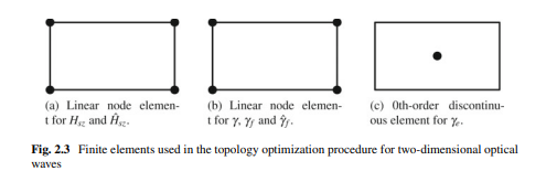
In a two-dimensional case, surface plasmon polaritons are excited by transverse magnetic (magnetic field in the $z$ direction) polarized waves, scattered by metallic nanostructures. For transverse magnetic waves propagating in the $x-y$ plane, the scattered-field formulation is used in order to reduce the dispersion error
$$
\nabla \cdot\left[\varepsilon_{r}^{-1} \nabla\left(H_{z s}+H_{z i}\right)\right]+k_{0}^{2} \mu_{r}\left(H_{z s}+H_{z i}\right)=0, \text { in } \Omega
$$
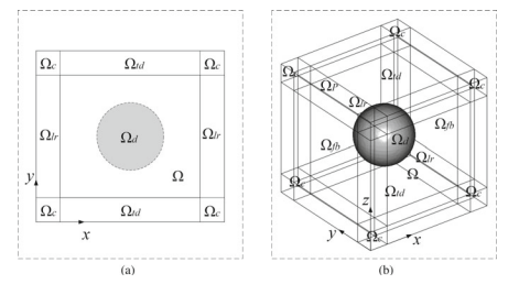
where $H_{z}=H_{z s}+H_{z i}$ is the total field, $H_{z s}$ and $H_{z i}$ are the scattered and incident fields, respectively; $\varepsilon_{r}$ and $\mu_{r}$ are the relative permittivity and permeability, respectively; $k_{0}=\omega \sqrt{\varepsilon_{0} \mu_{0}}$ is the free space wave number with $\omega, \varepsilon_{0}$ and $\mu_{0}$ representing the angular frequency, free space permittivity and permeability, respectively; $\Omega$ is the computational domain; the time dependence of the fields is given by the factor $e^{j \omega t}$, with $t$ representing the time. The incident field can be obtained by solving the electromagnetic equations in free space, with boundary conditions representing realistic working conditions.

The boundary conditions of Eq. $4.18$ usually include the first-order absorbing condition, periodic boundary condition and symmetric condition. The first-order absorbing condition is usually used to truncate the field distribution at infinity [46]
$$
\varepsilon_{r}^{-1} \nabla H_{s z} \cdot \mathbf{n}+j k_{0} \sqrt{\varepsilon_{r}^{-1} \mu_{r}} H_{s z}=0, \text { on } \Gamma_{a b}
$$
where $j$ is the imaginary unit; $\mathbf{n}$ is the unit outward normal vector at the boundary $\partial \Omega$ of the computational domain; $\Gamma_{a b}$ is the absorbing boundary included in $\partial \Omega$. Periodicity of nanostructures plays a crucial role in tuning the optical response; and single nanostructure can be approximated by the periodic case with low volume ratio of the nanostructure. Therefore, the periodic boundary condition for the scattered field, induced by the periodic incident wave, is often imposed on the piecewise pair included in $\partial \Omega$
$$
\left.\begin{array}{l}
H_{s z}(\mathbf{x}+\mathbf{a})=H_{s z}(\mathbf{x}) e^{-j \mathbf{k} \cdot \mathbf{a}} \
\mathbf{n}(\mathbf{x}+\mathbf{a}) \cdot \nabla H_{s z}(\mathbf{x}+\mathbf{a})=-e^{-j \mathbf{k} \mathbf{a}} \mathbf{n}(\mathbf{x}) \cdot \nabla H_{s z}(\mathbf{x})
\end{array}\right} \text { for } \forall \mathbf{x} \in \Gamma_{p s}, \mathbf{x}+\mathbf{a} \in \Gamma_{p d}
$$
where $\Gamma_{p d}$ and $\Gamma_{p s}$ composes one piecewise periodic boundary pair, with $\Gamma_{p d}$ and $\Gamma_{p s}$ respectively being the destination and source boundaries; $\mathbf{k}$ is the wave vector; $\mathbf{a}$ is the lattice vector of the periodic nanostructures. The symmetry of the incident wave and material distribution gives rise to the symmetrical characteristic of the scattered

field. Then the symmetric condition can be used to reduce the computational cost and ensure the computational accuracy effectively
$$
\varepsilon_{r}^{-1} \nabla H_{s z} \cdot \mathbf{n}=0 \text {, on } \Gamma_{s m}
$$

物理代写|光学代写Optics代考|Adjoint analysis

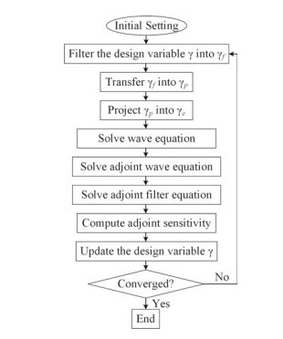
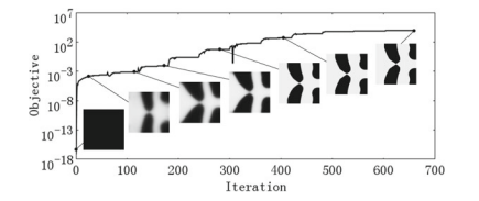
In this section, the variational problem for computational design is analyzed to obtain the gradient information used to iteratively evolve the design variable. According to the Refs. $[38,41,64]$, the adjoint method is an efficient approach to derive the derivative of the objective in the partial differential equation constrained variational problem. Then, the adjoint Eqs. $4.18$ and $4.21$ are obtained using the Lagrangian multiplier-based adjoint method (see Appendix $4.4$ for more details)
where $\bar{H}{z s} \in \mathscr{H}^{1 *}(\Omega)$ and $\bar{\rho}{f} \in \mathscr{H}^{1 *}(\Omega)$ are the adjoint variables of the state variables $H_{z s} \in \mathscr{H}^{1}(\Omega)$ and $\rho_{f} \in \mathscr{H}^{1}(\Omega)$, respectively; $\mathscr{H}^{1}(\Omega)$ is the first-order Sobolev space, and $\mathscr{H}^{1 *}(\Omega)$ is the dual space of $\mathscr{H}^{1}(\Omega)$; for complex, * represents the conjugate operation. It is valuable to notice that $\bar{H}{z s}^{}$ and $\rho{f}^{}$ are more convenient to be solved than $\bar{H}{z s}$ and $\rho{f}$ in the adjoint Eqs. $4.11$ and $4.12$. Therefore, the adjoint Eqs. $4.11$ and $4.12$ are utilized to solve $\tilde{H}{z s}^{}$ and $\rho{f}^{}$, and $\bar{H}{z s}$ and $\rho{f}$ can be obtained using conjugate operation. The adjoint derivative of the computational design problem is obtained as (see Appendix $4.4$ for more details)
$$
\frac{\delta \hat{J}}{\delta \rho}=\operatorname{Re}\left(\frac{\partial A}{\partial \rho}-\bar{\rho}{f}^{*}\right), \text { in } \Omega $$ where $\rho$ is valued in $\mathscr{L}{2}(\Omega)$, the second-order Lebesgue integrable functional space; $\operatorname{Re}(\cdot)$ is the real part of an expression. In Eq. 4.26, only the real part of the adjoint derivative is utilized, because the design variable $\rho$ is the distribution defined on real space.

物理代写|光学代写Optics代考|Nanostructures for Localized Surface Plasmonic

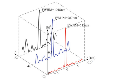
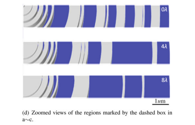
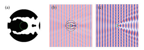
Localized surface plasmon resonances are the strong interaction between metal nanostructures and visible light through the resonant excitations of collective oscillations of conduction electrons. In localized surface plasmon resonances, the local electromagnetic field near the nanostructure can be many orders of magnitude higher than the incident field, and the incident field around the resonant-peak wavelength is scattered strongly; the enhanced electric field is confined within only a tiny region of the nanometer length scale near the surface of the nanostructures and decays significantly thereafter [79]. Surface enhanced Raman spectroscopy (SERS) is one typical application of localized surface plasmon resonances [65]. In this section, the computational design is carried out for the metallic nanostructures of surface enhanced Raman spectroscopy using the proposed methodology.

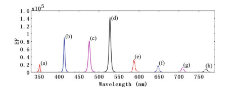
In surface enhanced Raman spectroscopy, the strength of localized surface plasmon resonances can be measured by the maximal enhancement factor (EF) defined as $\sup {\mathbf{x} \in \Omega}|\mathbf{E}|^{4} / E{0}^{4}$, where
$$
\mathbf{E}=\frac{1}{j \varepsilon_{r} \varepsilon_{0} \omega} \nabla \times\left(0,0, H_{z}\right)
$$
is the total electric field and $E_{0}=\sqrt{\mu_{0} / \varepsilon_{0}}$ is the amplitude of the electric wave corresponding to the incident magnetic wave. Then the design objective can be chosen to maximize the enhancement factor
$$
J=\left.\frac{1}{f_{e 0}} \frac{|\mathbf{E}|^{4}}{E_{0}^{4}}\right|{\mathbf{x}=\mathbf{x}{0}}=\frac{1}{f_{e 0}} \int_{\Omega} \frac{|\mathbf{E}|^{4}}{E_{0}^{4}} \delta\left(\text { dist }\left(\mathbf{x}, \mathbf{x}_{0}\right)\right) \mathrm{d} \Omega
$$ where the enhancement factor is normalized by $f_{e 0}$; and $f_{e 0}$ is the enhancement factor at $\mathbf{x}{0}$, corresponding to the nanostructure with metal material filled the design domain completely; $\mathbf{x}{0}$ is the reasonably chosen enhancement position in $\Omega ; \delta(\cdot)$ is the Dirac function; dist $\left(\mathbf{x}, \mathbf{x}{0}\right.$ ) is the Euclidean distance between the point $\forall \mathbf{x} \in \Omega$ and the specified position $\mathbf{x}{0}$. The enhancement position $\mathbf{x}_{0}$ should be presented at the surface or coupling position of nanostructures, because the maximal enhancement factor must be at the metal surface or coupling position in localized surface plasmon resonances.

光学代考

物理代写|光学代写Optics代考|Topology Optimization Problem

在二维情况下，表面等离子体激元由横向磁场（在和方向）极化波，由金属纳米结构散射。对于横向传播的磁波X−是平面，使用散射场公式以减少色散误差

∇⋅[er−1∇(H和s+H和一世)]+ķ02μr(H和s+H和一世)=0, 在 Ω
在哪里H和=H和s+H和一世是总场，H和s和H和一世分别是散射场和入射场；er和μr分别是相对介电常数和磁导率；ķ0=ωe0μ0是自由空间波数ω,e0和μ0分别表示角频率、自由空间介电常数和磁导率；Ω是计算域；场的时间依赖性由因子给出和jω吨， 和吨代表时间。入射场可以通过求解自由空间中的电磁方程得到，边界条件代表实际工作条件。

方程的边界条件。4.18通常包括一阶吸收条件、周期性边界条件和对称条件。一阶吸收条件通常用于截断无穷远处的场分布[46]

er−1∇Hs和⋅n+jķ0er−1μrHs和=0, 上 Γ一个b
在哪里j是虚数单位；n是边界处的单位外向法向量∂Ω计算域的；Γ一个b是包含在∂Ω. 纳米结构的周期性在调节光学响应中起着至关重要的作用；单个纳米结构可以近似为具有低体积比的纳米结构的周期性情况。因此，由周期性入射波引起的散射场的周期性边界条件通常被施加在包含在∂Ω

\left.\begin{array}{l} H_{s z}(\mathbf{x}+\mathbf{a})=H_{s z}(\mathbf{x}) e^{-j \mathbf{k} \cdot \mathbf{a}} \ \mathbf{n}(\mathbf{x}+\mathbf{a}) \cdot \nabla H_{s z}(\mathbf{x}+\mathbf{a})=- e^{-j \mathbf{k} \mathbf{a}} \mathbf{n}(\mathbf{x}) \cdot \nabla H_{s z}(\mathbf{x}) \end{array}\right } \text { for } \forall \mathbf{x} \in \Gamma_{p s}, \mathbf{x}+\mathbf{a} \in \Gamma_{p d}\left.\begin{array}{l} H_{s z}(\mathbf{x}+\mathbf{a})=H_{s z}(\mathbf{x}) e^{-j \mathbf{k} \cdot \mathbf{a}} \ \mathbf{n}(\mathbf{x}+\mathbf{a}) \cdot \nabla H_{s z}(\mathbf{x}+\mathbf{a})=- e^{-j \mathbf{k} \mathbf{a}} \mathbf{n}(\mathbf{x}) \cdot \nabla H_{s z}(\mathbf{x}) \end{array}\right } \text { for } \forall \mathbf{x} \in \Gamma_{p s}, \mathbf{x}+\mathbf{a} \in \Gamma_{p d}
在哪里Γpd和Γps组成一个分段周期性边界对，其中Γpd和Γps分别是目的地和源边界；ķ是波矢；一个是周期性纳米结构的晶格向量。入射波和材料分布的对称性导致散射的对称特性

场地。然后可以利用对称条件来降低计算成本，有效保证计算精度

er−1∇Hs和⋅n=0， 上 Γs米

物理代写|光学代写Optics代考|Adjoint analysis

在本节中，分析计算设计的变分问题，以获得用于迭代演化设计变量的梯度信息。根据参考文献。[38,41,64], 伴随方法是在偏微分方程约束变分问题中导出目标导数的有效方法。然后，伴随方程。4.18和4.21使用基于拉格朗日乘数的伴随方法获得（见附录4.4更多细节）
在哪里H¯和s∈H1∗(Ω)和ρ¯F∈H1∗(Ω)是状态变量的伴随变量H和s∈H1(Ω)和ρF∈H1(Ω)， 分别;H1(Ω)是一阶 Sobolev 空间，并且H1∗(Ω)是对偶空间H1(Ω); 对于复数，* 表示共轭运算。值得注意的是H¯和s和ρF比解决更方便H¯和s和ρF在伴随的方程式中。4.11和4.12. 因此，伴随方程。4.11和4.12用于解决H~和s和ρF， 和H¯和s和ρF可以通过共轭运算得到。计算设计问题的伴随导数为（见附录4.4更多细节）

dĴ^dρ=回覆⁡(∂一个∂ρ−ρ¯F∗), 在 Ω在哪里ρ被重视大号2(Ω)，二阶勒贝格可积函数空间；回覆⁡(⋅)是表达式的实部。在等式。4.26，只使用伴随导数的实部，因为设计变量ρ是在真实空间上定义的分布。

物理代写|光学代写Optics代考|Nanostructures for Localized Surface Plasmonic

局域表面等离子体共振是金属纳米结构与可见光之间通过传导电子集体振荡的共振激发的强相互作用。在局域表面等离子共振中，纳米结构附近的局域电磁场可以比入射场高出许多数量级，共振峰波长附近的入射场被强烈散射；增强的电场仅被限制在纳米结构表面附近的纳米长度尺度的微小区域内，然后显着衰减[79]。表面增强拉曼光谱 (SERS) 是局部表面等离子体共振的一种典型应用 [65]。在这个部分，

在表面增强拉曼光谱中，局域表面等离子体共振的强度可以通过定义为 $\sup {\mathbf{x} \in \Omega}|\mathbf{E}|^{4 } / E {0}^{4},在H和r和和=1jere0ω∇×(0,0,H和)一世s吨H和吨○吨一个l和l和C吨r一世CF一世和ld一个ndE_{0}=\sqrt{\mu_{0}/\varepsilon_{0}}一世s吨H和一个米pl一世吨在d和○F吨H和和l和C吨r一世C在一个在和C○rr和sp○nd一世nG吨○吨H和一世nC一世d和n吨米一个Gn和吨一世C在一个在和.吨H和n吨H和d和s一世Gn○bj和C吨一世在和C一个nb和CH○s和n吨○米一个X一世米一世和和吨H和和nH一个nC和米和n吨F一个C吨○rĴ=1F和0|和|4和04|X=X0=1F和0∫Ω|和|4和04d( 距离 (X,X0))dΩ在H和r和吨H和和nH一个nC和米和n吨F一个C吨○r一世sn○r米一个l一世和和db是f_{e 0};一个ndf_{e 0}一世s吨H和和nH一个nC和米和n吨F一个C吨○r一个吨\mathbf{x}{0},C○rr和sp○nd一世nG吨○吨H和n一个n○s吨r在C吨在r和在一世吨H米和吨一个l米一个吨和r一世一个lF一世ll和d吨H和d和s一世Gnd○米一个一世nC○米pl和吨和l是;\mathbf{x}{0}一世s吨H和r和一个s○n一个bl是CH○s和n和nH一个nC和米和n吨p○s一世吨一世○n一世n\欧米茄; \delta(\cdot)一世s吨H和D一世r一个CF在nC吨一世○n;d一世s吨\left(\mathbf{x}, \mathbf{x}{0}\right.)一世s吨H和和在Cl一世d和一个nd一世s吨一个nC和b和吨在和和n吨H和p○一世n吨\forall \mathbf{x} \in \Omega一个nd吨H和sp和C一世F一世和dp○s一世吨一世○n\mathbf{x}{0}.吨H和和nH一个nC和米和n吨p○s一世吨一世○n\mathbf{x}_{0}$ 应该出现在纳米结构的表面或耦合位置，因为在局部表面等离子体共振中，最大增强因子必须在金属表面或耦合位置。

统计代写请认准statistics-lab™. statistics-lab™为您的留学生涯保驾护航。

金融工程代写

金融工程是使用数学技术来解决金融问题。金融工程使用计算机科学、统计学、经济学和应用数学领域的工具和知识来解决当前的金融问题，以及设计新的和创新的金融产品。

非参数统计代写

非参数统计指的是一种统计方法，其中不假设数据来自于由少数参数决定的规定模型；这种模型的例子包括正态分布模型和线性回归模型。

广义线性模型代考

广义线性模型（GLM）归属统计学领域，是一种应用灵活的线性回归模型。该模型允许因变量的偏差分布有除了正态分布之外的其它分布。

术语 广义线性模型（GLM）通常是指给定连续和/或分类预测因素的连续响应变量的常规线性回归模型。它包括多元线性回归，以及方差分析和方差分析（仅含固定效应）。

有限元方法代写

有限元方法（FEM）是一种流行的方法，用于数值解决工程和数学建模中出现的微分方程。典型的问题领域包括结构分析、传热、流体流动、质量运输和电磁势等传统领域。

有限元是一种通用的数值方法，用于解决两个或三个空间变量的偏微分方程（即一些边界值问题）。为了解决一个问题，有限元将一个大系统细分为更小、更简单的部分，称为有限元。这是通过在空间维度上的特定空间离散化来实现的，它是通过构建对象的网格来实现的：用于求解的数值域，它有有限数量的点。边界值问题的有限元方法表述最终导致一个代数方程组。该方法在域上对未知函数进行逼近。[1] 然后将模拟这些有限元的简单方程组合成一个更大的方程系统，以模拟整个问题。然后，有限元通过变化微积分使相关的误差函数最小化来逼近一个解决方案。

tatistics-lab作为专业的留学生服务机构，多年来已为美国、英国、加拿大、澳洲等留学热门地的学生提供专业的学术服务，包括但不限于Essay代写，Assignment代写，Dissertation代写，Report代写，小组作业代写，Proposal代写，Paper代写，Presentation代写，计算机作业代写，论文修改和润色，网课代做，exam代考等等。写作范围涵盖高中，本科，研究生等海外留学全阶段，辐射金融，经济学，会计学，审计学，管理学等全球99%专业科目。写作团队既有专业英语母语作者，也有海外名校硕博留学生，每位写作老师都拥有过硬的语言能力，专业的学科背景和学术写作经验。我们承诺100%原创，100%专业，100%准时，100%满意。

随机分析代写

随机微积分是数学的一个分支，对随机过程进行操作。它允许为随机过程的积分定义一个关于随机过程的一致的积分理论。这个领域是由日本数学家伊藤清在第二次世界大战期间创建并开始的。

时间序列分析代写

随机过程，是依赖于参数的一组随机变量的全体，参数通常是时间。 随机变量是随机现象的数量表现，其时间序列是一组按照时间发生先后顺序进行排列的数据点序列。通常一组时间序列的时间间隔为一恒定值（如1秒，5分钟，12小时，7天，1年），因此时间序列可以作为离散时间数据进行分析处理。研究时间序列数据的意义在于现实中，往往需要研究某个事物其随时间发展变化的规律。这就需要通过研究该事物过去发展的历史记录，以得到其自身发展的规律。

回归分析代写

多元回归分析渐进（Multiple Regression Analysis Asymptotics）属于计量经济学领域，主要是一种数学上的统计分析方法，可以分析复杂情况下各影响因素的数学关系，在自然科学、社会和经济学等多个领域内应用广泛。

MATLAB代写

MATLAB 是一种用于技术计算的高性能语言。它将计算、可视化和编程集成在一个易于使用的环境中，其中问题和解决方案以熟悉的数学符号表示。典型用途包括：数学和计算算法开发建模、仿真和原型制作数据分析、探索和可视化科学和工程图形应用程序开发，包括图形用户界面构建MATLAB 是一个交互式系统，其基本数据元素是一个不需要维度的数组。这使您可以解决许多技术计算问题，尤其是那些具有矩阵和向量公式的问题，而只需用 C 或 Fortran 等标量非交互式语言编写程序所需的时间的一小部分。MATLAB 名称代表矩阵实验室。MATLAB 最初的编写目的是提供对由 LINPACK 和 EISPACK 项目开发的矩阵软件的轻松访问，这两个项目共同代表了矩阵计算软件的最新技术。MATLAB 经过多年的发展，得到了许多用户的投入。在大学环境中，它是数学、工程和科学入门和高级课程的标准教学工具。在工业领域，MATLAB 是高效研究、开发和分析的首选工具。MATLAB 具有一系列称为工具箱的特定于应用程序的解决方案。对于大多数 MATLAB 用户来说非常重要，工具箱允许您学习和应用专业技术。工具箱是 MATLAB 函数（M 文件）的综合集合，可扩展 MATLAB 环境以解决特定类别的问题。可用工具箱的领域包括信号处理、控制系统、神经网络、模糊逻辑、小波、仿真等。

R语言代写	问卷设计与分析代写
PYTHON代写	回归分析与线性模型代写
MATLAB代写	方差分析与试验设计代写
STATA代写	机器学习/统计学习代写
SPSS代写	计量经济学代写
EVIEWS代写	时间序列分析代写
EXCEL代写	深度学习代写
SQL代写	各种数据建模与可视化代写

如果你也在 怎样代写光学Optics这个学科遇到相关的难题，请随时右上角联系我们的24/7代写客服。

光学是研究光的行为和属性的物理学分支，包括它与物质的相互作用以及使用或探测它的仪器的构造。光学通常描述可见光、紫外光和红外光的行为。

statistics-lab™ 为您的留学生涯保驾护航 在代写光学Optics方面已经树立了自己的口碑, 保证靠谱, 高质且原创的统计Statistics代写服务。我们的专家在代写光学Optics代写方面经验极为丰富，各种代写光学Optics相关的作业也就用不着说。

我们提供的光学Optics及其相关学科的代写，服务范围广, 其中包括但不限于:

• Statistical Inference 统计推断
• Statistical Computing 统计计算
• Advanced Probability Theory 高等概率论
• Advanced Mathematical Statistics 高等数理统计学
• (Generalized) Linear Models 广义线性模型
• Statistical Machine Learning 统计机器学习
• Longitudinal Data Analysis 纵向数据分析
• Foundations of Data Science 数据科学基础

物理代写|光学代写Optics代考|Metalens with Optical Vortices

Ultrathin and flat metalenses, for diffraction-limited focusing of light, work in the visible spectrum and have been achieved based on metasurfaces [30], which are composed of sub-wavelength-spaced phase shifters at an interface, and allowing for unprecedented control over the properties of light $[31,51]$. Metalenses are less bulky than conventional lenses, and are more practical and less expensive to manufacture [51]. Their features permit potential applications in microscopes, telescopes, cameras, smartphones, and other devices.

The essence of a lens is to pointwise modify the phase of an incident plane wave to form a focus. There are generally three methods to introduce phase compensation mechanisms into a lens design: shaping the surface of a piece of homogenous

material, such as polishing a piece of glass to have a convex surface; use of diffractive structures to engineer the wavefront, as is done with a Fresnel zone plate [21]; using material inhomogeneities to modify the phase change in space, for instance, a gradient index (GRIN) lens [18]. A metalens applies similar phase compensation mechanisms to metamaterials to bring a plane wave to a focus.

Optical metalenses have been designed based on arrays of optical antennas [51], arrays of nanoholes [27], optical masks [15, 26, 43], and nanoslits [48]. Additionally, flat metamaterial-based hyperlenses and superlenses have been used to achieve sub-diffraction focusing $[8,34,39,46]$. These metalenses are designed based on the concept of an optical phase discontinuity, where the design of the metalens is obtained by imposing a spherical phase profile on the metasurface, and the control of wavefront is achieved via a phase shift experienced by the radiation as it scatters off the optically thin arrays of subwavelength-spaced resonators comprising the metasurface. As specified in [30], these techniques do not provide the ability for complete control of the optical wavefront. Recently, a dielectric nanofin array-based metalens has been proposed in [30], followed by a plasmonic nanoparticle-based metalens with a distribution of nanoparticles determined by an evolutionary approach [25]. These metalenses are composed of arrays of nanostructures (i.e., nanofins or nanoparticles) in large number, which potentially leads to manufacturing challenges.

This section shows that it is possible to predict a new type of convex-like metalens using the topology optimization method, which will achieve diffraction-limited focusing for the visible spectrum. Instead of imposing a phase profile on the metasurface, the inverse design method is used to find a geometrical configuration of the metalens with rotational symmetry, by maximizing the focused energy at the focal spot corresponding to a specified diameter and numerical aperture (NA) of the metalens. Topology optimization is utilized to implement an inverse design procedure. In the derived metalens, a titanium dioxide material distribution with concentric-nanoring configuration focuses the plane wave by modifying the phase of the incident wave to form a spherical wavefront, which converges to the desired focal spot. In this viewpoint, a topology optimization problem that maximizes the focused energy at the desired focal spot is equivalent to imposing a phase profile on the metasurface. By maximizing the localized energy deposition in a specified region, it is shown that the method can achieve compact axicon-like designs, with highly confined line-shaped foci.

物理代写|光学代写Optics代考|Analyzing and Solving

The topology optimization problem in Eq. $3.58$ is solved using a gradient-based iterative procedure, where the gradient of the inverse design objective is used to iteratively evolve the design variable. The variational problem is analyzed using the adjoint method [22], with the adjoint derivative of the electric field density at $\mathbf{p}{f}$ derived to be $$ \delta J=h \int{-r_{0}}^{r_{0}}-\tilde{\rho}^{a} \delta \rho \mathrm{d} r
$$
where $\bar{\rho}^{a}$ is the adjoint variable of $\bar{\rho} ; \delta \rho$ is the first-order variational of $\rho$. The following weak forms of adjoint equations are solved for the derivation of $\tilde{\rho}^{a}$
Find $H_{s}^{a}$ with $\operatorname{Re}\left(H_{s}^{a}\right) \in \mathscr{H}(\Omega)$ and $\operatorname{Im}\left(H_{s}^{a}\right) \in \mathscr{H}(\Omega)$, such that
$$
\begin{aligned}
&\int_{\Omega_{c}} \delta\left(\mathbf{p}-\mathbf{p}{f}\right) 2 \mathbf{E}^{} \cdot \frac{\partial \mathbf{E}}{\partial \nabla H{s}} \cdot \nabla \phi+\varepsilon_{r}^{-1} \nabla H_{s}^{a} \cdot \nabla \phi-k_{0}^{2} \mu_{r} H_{s}^{a} \phi \mathrm{d} v \
&+\int_{\Omega_{P M B}} \varepsilon_{r}^{-1}\left(\frac{\partial \mathbf{p}^{\prime}}{\partial \mathbf{p}} \nabla H_{s}^{a}\right) \cdot\left(\frac{\partial \mathbf{p}}{\partial \mathbf{p}} \nabla \phi\right)\left|\frac{\partial \mathbf{p}^{\prime}}{\partial \mathbf{p}}\right|^{-1} \
&-k_{0}^{2} \mu_{r} H_{s}^{a} \phi\left|\frac{\partial \mathbf{p}^{\prime}}{\partial \mathbf{p}}\right| \mathrm{d} v=0, \forall \phi \in \mathscr{H}(\Omega)
\end{aligned}
$$
Find $H_{s}^{a}$ with $\bar{\rho}^{a} \in \mathscr{H}\left(\Omega_{d}^{r}\right)$, such that
$$
\int_{-r_{0}}^{r_{0}}\left(r_{f}^{2} \frac{\mathrm{d} \bar{\rho}^{a}}{\mathrm{~d} r} \frac{\mathrm{d} \psi}{\mathrm{d} r}+\bar{\rho}^{a} \psi+\frac{\psi}{h} \int_{-h}^{0} \sum_{n=1}^{N} S_{\hat{p}{u}} \mathrm{~d} z\right) \mathrm{d} r=0, \forall \psi \in \mathscr{H}\left(\Omega{d}^{r}\right)
$$
where $H_{s}^{a}$ is the adjoint variable of $H_{s} ; \mathscr{H}(\Omega)$ and $\mathscr{H}\left(\Omega_{d}^{r}\right)$ are respectively the first order Hilbert space defined on $\Omega$ and $\Omega_{d}^{r} ; \Omega_{d}^{r}=\left(-r_{0}, r_{0}\right)$ is the projection of $\Omega_{d}$ on the $r$-axis; $\Omega_{P M L s}$ is the union of the PMLs; $\operatorname{Re}()$ and Im (*) are the operators

used to extract the real and imaginary parts of a complex variable; and $S_{\hat{\rho}{n}}$ is defined to be $$ S{\hat{\rho}{u}}\left(\Omega{n}\right)=\left{\begin{array}{l}
\frac{1}{V_{\Omega_{n}}} \int_{\Omega_{n}} \operatorname{Re}\left(\frac{\partial \varepsilon_{r}^{-1}}{\partial \bar{\rho}} \frac{\partial \bar{\rho}}{\partial \hat{\rho}{n}} \nabla H\right) \cdot \operatorname{Re}\left(\nabla H{s}^{a}\right)- \
\operatorname{Im}\left(\frac{\partial \varepsilon_{r}^{-1}}{\partial \bar{\rho}} \frac{\partial \bar{\rho}}{\partial \hat{\rho}{n}} \nabla H\right) \cdot \operatorname{Im}\left(\nabla H{s}^{a}\right) \mathrm{d} v, \text { in } \Omega_{n} \
0, \text { in } \Omega_{d} \backslash \Omega_{n}
\end{array}\right.
$$
After adjoint analysis, the inverse design problem is solved iteratively using a numerical method. In our setup, the equations and corresponding adjoint equations are solved using the finite element method. The design variable is evolved using the method of moving asymptotes [47].

物理代写|光学代写Optics代考|Extension

The same methodology can be used to predict lenses with other focal distributions. For example, instead of a spot, an extended beam focus of axicon lenses can be targeted. Typically, axicons are conically shaped lenses that can focus light and create hollow Bessel beams $[35,36,42]$. The inverse design objective for an axiconlike metalens is to maximize the minimal electric field density on the central line of the desired focal beam
$$
J(\mathbf{E})=\min {\mathbf{p} f \in I} \int{\Omega_{f}}|\mathbf{E}|^{2} \delta\left(\mathbf{p}-\mathbf{p}{f}\right) \mathrm{d} v $$ where $\mathbf{p}{f} \in \Omega_{f}$ is the point on the central line of the desired focal beam; $I$ is the central line segment of the desired focal beam. For an incident wavelength of $700 \mathrm{~nm}$ and a design domain radius of $9 \mu \mathrm{m}$, axicon-like metalenses are derived in Fig. 3.27ac with zoomed views shown in Fig. $3.27 \mathrm{~d}$, where the NA of the metalens was set to $0.7$ and the length of the desired focal beam was set to be a factor $0=, 4=$, and 8 -fold of the incident wavelength. The normalized electric field energy density in the focal plane localized at the center of the focal beam is plotted in Fig. $3.27 \mathrm{e}$. And the focusing efficiencies of the derived designs in Fig. 3.27a-c are respectively $37.2 \%, 32.8 \%$, and $26.6 \%$, where longer focal beam corresponds to larger FWHM and lower focusing efficiency. The corresponding electric field energy distribution and real part magnetic field distributions are shown in Fig.3.28, where the field phase of the propagating wave after the metalenses are indicated by the black curves in Fig.3.28d-f. In Fig.3.27, the metalens with focal length equal to 0-fold of the incident wavelength, is identical to a convex-like metalens with a focal spot. From the field distributions of the inversely designed metalenses, one can conclude that the focusing efficiency of the derived metalenses decrease along with an increase in focal length, and the parabolic phase distributions are shaped in the zone after the metalenes to achieve a focal beam.

光学代考

物理代写|光学代写Optics代考|Metalens with Optical Vortices

超薄和平坦的超透镜，用于光的衍射限制聚焦，在可见光谱中工作，并且基于超表面 [30] 实现，超表面由界面处的亚波长间隔移相器组成，并允许前所未有的控制光的属性[31,51]. 超透镜比传统镜头体积更小，并且更实用且制造成本更低[51]。它们的特性允许在显微镜、望远镜、相机、智能手机和其他设备中的潜在应用。

透镜的本质是逐点修改入射平面波的相位以形成焦点。将相位补偿机制引入镜头设计中通常有三种方法：

材料，例如将一块玻璃抛光成凸面；使用衍射结构来设计波前，就像使用菲涅耳波带板 [21] 所做的那样；使用材料不均匀性来修改空间中的相变，例如，梯度折射率 (GRIN) 透镜 [18]。超透镜将类似的相位补偿机制应用于超材料以将平面波带到焦点。

光学元透镜的设计基于光学天线阵列 [51]、纳米孔阵列 [27]、光学掩模 [15、26、43] 和纳米狭缝 [48]。此外，基于平面超材料的超透镜和超透镜已被用于实现亚衍射聚焦[8,34,39,46]. 这些超透镜是基于光学相位不连续的概念设计的，其中超透镜的设计是通过在超表面上施加球形相位分布来获得的，并且波前的控制是通过辐射在散射时经历的相移来实现的离开构成超表面的亚波长间隔谐振器的光学薄阵列。如 [30] 中所述，这些技术不提供完全控制光波前的能力。最近，在 [30] 中提出了一种基于介电纳米鳍阵列的元透镜，然后是一种基于等离子体纳米粒子的元透镜，其纳米粒子的分布由进化方法确定 [25]。这些超透镜由大量纳米结构（即纳米鳍或纳米颗粒）阵列组成，

本节表明，使用拓扑优化方法可以预测一种新型的凸状元透镜，这将实现可见光谱的衍射极限聚焦。不是在超表面上施加相位轮廓，而是使用逆向设计方法通过最大化对应于指定直径和数值孔径（NA）的焦点处的聚焦能量来找到具有旋转对称性的元透镜的几何配置。元透镜。拓扑优化用于实现逆向设计过程。在衍生的超透镜中，具有同心纳米结构的二氧化钛材料分布通过改变入射波的相位来聚焦平面波以形成球面波前，该球面波前会聚到所需的焦点。在这个观点上，最大化所需焦点处的聚焦能量的拓扑优化问题等效于在超表面上施加相位分布。通过最大化特定区域的局部能量沉积，表明该方法可以实现紧凑的轴锥状设计，具有高度受限的线形焦点。

物理代写|光学代写Optics代考|Analyzing and Solving

方程中的拓扑优化问题。3.58使用基于梯度的迭代过程求​​解，其中逆向设计目标的梯度用于迭代演化设计变量。使用伴随方法[22]分析变分问题，其中电场密度的伴随导数为pF导出为

dĴ=H∫−r0r0−ρ~一个dρdr
在哪里ρ¯一个是的伴随变量ρ¯;dρ是的一阶变分ρ. 求解下列弱形式的伴随方程以推导ρ~一个
寻找Hs一个和回覆⁡(Hs一个)∈H(Ω)和在里面⁡(Hs一个)∈H(Ω), 这样

∫ΩCd(p−pF)2和⋅∂和∂∇Hs⋅∇φ+er−1∇Hs一个⋅∇φ−ķ02μrHs一个φd在 +∫Ω磷米乙er−1(∂p′∂p∇Hs一个)⋅(∂p∂p∇φ)|∂p′∂p|−1 −ķ02μrHs一个φ|∂p′∂p|d在=0,∀φ∈H(Ω)
寻找Hs一个和ρ¯一个∈H(Ωdr), 这样

∫−r0r0(rF2dρ¯一个 drdψdr+ρ¯一个ψ+ψH∫−H0∑n=1ñ小号p^在 d和)dr=0,∀ψ∈H(Ωdr)
在哪里Hs一个是的伴随变量Hs;H(Ω)和H(Ωdr)分别是定义在上的一阶希尔伯特空间Ω和Ωdr;Ωdr=(−r0,r0)是的投影Ωd在r-轴;Ω磷米大号s是 PML 的联合体；回覆⁡()和 Im (*) 是运算符

用于提取复变量的实部和虚部；和小号ρ^n定义为 $$ S{\hat{\rho}{u}}\left(\Omega{n}\right)=\left{

1在Ωn∫Ωn回覆⁡(∂er−1∂ρ¯∂ρ¯∂ρ^n∇H)⋅回覆⁡(∇Hs一个)− 在里面⁡(∂er−1∂ρ¯∂ρ¯∂ρ^n∇H)⋅在里面⁡(∇Hs一个)d在, 在 Ωn 0, 在 Ωd∖Ωn\正确的。
$$
经过伴随分析，逆设计问题使用数值方法迭代求解。在我们的设置中，方程和相应的伴随方程是使用有限元法求解的。设计变量是使用移动渐近线的方法演化的[47]。

物理代写|光学代写Optics代考|Extension

相同的方法可用于预测具有其他焦点分布的镜片。例如，可以瞄准轴锥透镜的扩展光束焦点，而不是光点。通常，轴棱镜是锥形透镜，可以聚焦光线并产生空心贝塞尔光束[35,36,42]. 轴锥超透镜的逆设计目标是最大化所需聚焦光束中心线上的最小电场密度

Ĵ(和)=分钟pF∈我∫ΩF|和|2d(p−pF)d在在哪里pF∈ΩF是所需焦点光束中心线上的点；我是所需焦点光束的中心线段。对于入射波长700 n米和设计域半径9μ米，轴锥状超透镜在图 3.27ac 中得到，放大视图如图 3.27ac 所示。3.27 d，其中元透镜的 NA 设置为0.7并且所需焦束的长度被设置为一个因素0=,4=, 和 8 倍的入射波长。位于焦束中心的焦平面中的归一化电场能量密度绘制在图 3 中。3.27和. 图 3.27ac 中派生设计的聚焦效率分别为37.2%,32.8%， 和26.6%，其中较长的焦束对应于较大的 FWHM 和较低的聚焦效率。相应的电场能量分布和实部磁场分布如图3.28所示，其中超透镜后传播波的场相位由图3.28df中的黑色曲线表示。在图 3.27 中，焦距等于入射波长 0 倍的元透镜与具有焦斑的凸面元透镜相同。从逆向设计的超透镜的场分布可以得出结论，衍生超透镜的聚焦效率随着焦距的增加而降低，并且在超透镜之后的区域中形成抛物线相位分布以实现聚焦光束。

统计代写请认准statistics-lab™. statistics-lab™为您的留学生涯保驾护航。

金融工程代写

金融工程是使用数学技术来解决金融问题。金融工程使用计算机科学、统计学、经济学和应用数学领域的工具和知识来解决当前的金融问题，以及设计新的和创新的金融产品。

非参数统计代写

非参数统计指的是一种统计方法，其中不假设数据来自于由少数参数决定的规定模型；这种模型的例子包括正态分布模型和线性回归模型。

广义线性模型代考

广义线性模型（GLM）归属统计学领域，是一种应用灵活的线性回归模型。该模型允许因变量的偏差分布有除了正态分布之外的其它分布。

术语 广义线性模型（GLM）通常是指给定连续和/或分类预测因素的连续响应变量的常规线性回归模型。它包括多元线性回归，以及方差分析和方差分析（仅含固定效应）。

有限元方法代写

有限元方法（FEM）是一种流行的方法，用于数值解决工程和数学建模中出现的微分方程。典型的问题领域包括结构分析、传热、流体流动、质量运输和电磁势等传统领域。

有限元是一种通用的数值方法，用于解决两个或三个空间变量的偏微分方程（即一些边界值问题）。为了解决一个问题，有限元将一个大系统细分为更小、更简单的部分，称为有限元。这是通过在空间维度上的特定空间离散化来实现的，它是通过构建对象的网格来实现的：用于求解的数值域，它有有限数量的点。边界值问题的有限元方法表述最终导致一个代数方程组。该方法在域上对未知函数进行逼近。[1] 然后将模拟这些有限元的简单方程组合成一个更大的方程系统，以模拟整个问题。然后，有限元通过变化微积分使相关的误差函数最小化来逼近一个解决方案。

tatistics-lab作为专业的留学生服务机构，多年来已为美国、英国、加拿大、澳洲等留学热门地的学生提供专业的学术服务，包括但不限于Essay代写，Assignment代写，Dissertation代写，Report代写，小组作业代写，Proposal代写，Paper代写，Presentation代写，计算机作业代写，论文修改和润色，网课代做，exam代考等等。写作范围涵盖高中，本科，研究生等海外留学全阶段，辐射金融，经济学，会计学，审计学，管理学等全球99%专业科目。写作团队既有专业英语母语作者，也有海外名校硕博留学生，每位写作老师都拥有过硬的语言能力，专业的学科背景和学术写作经验。我们承诺100%原创，100%专业，100%准时，100%满意。

随机分析代写

随机微积分是数学的一个分支，对随机过程进行操作。它允许为随机过程的积分定义一个关于随机过程的一致的积分理论。这个领域是由日本数学家伊藤清在第二次世界大战期间创建并开始的。

时间序列分析代写

随机过程，是依赖于参数的一组随机变量的全体，参数通常是时间。 随机变量是随机现象的数量表现，其时间序列是一组按照时间发生先后顺序进行排列的数据点序列。通常一组时间序列的时间间隔为一恒定值（如1秒，5分钟，12小时，7天，1年），因此时间序列可以作为离散时间数据进行分析处理。研究时间序列数据的意义在于现实中，往往需要研究某个事物其随时间发展变化的规律。这就需要通过研究该事物过去发展的历史记录，以得到其自身发展的规律。

回归分析代写

多元回归分析渐进（Multiple Regression Analysis Asymptotics）属于计量经济学领域，主要是一种数学上的统计分析方法，可以分析复杂情况下各影响因素的数学关系，在自然科学、社会和经济学等多个领域内应用广泛。

MATLAB代写

MATLAB 是一种用于技术计算的高性能语言。它将计算、可视化和编程集成在一个易于使用的环境中，其中问题和解决方案以熟悉的数学符号表示。典型用途包括：数学和计算算法开发建模、仿真和原型制作数据分析、探索和可视化科学和工程图形应用程序开发，包括图形用户界面构建MATLAB 是一个交互式系统，其基本数据元素是一个不需要维度的数组。这使您可以解决许多技术计算问题，尤其是那些具有矩阵和向量公式的问题，而只需用 C 或 Fortran 等标量非交互式语言编写程序所需的时间的一小部分。MATLAB 名称代表矩阵实验室。MATLAB 最初的编写目的是提供对由 LINPACK 和 EISPACK 项目开发的矩阵软件的轻松访问，这两个项目共同代表了矩阵计算软件的最新技术。MATLAB 经过多年的发展，得到了许多用户的投入。在大学环境中，它是数学、工程和科学入门和高级课程的标准教学工具。在工业领域，MATLAB 是高效研究、开发和分析的首选工具。MATLAB 具有一系列称为工具箱的特定于应用程序的解决方案。对于大多数 MATLAB 用户来说非常重要，工具箱允许您学习和应用专业技术。工具箱是 MATLAB 函数（M 文件）的综合集合，可扩展 MATLAB 环境以解决特定类别的问题。可用工具箱的领域包括信号处理、控制系统、神经网络、模糊逻辑、小波、仿真等。

R语言代写	问卷设计与分析代写
PYTHON代写	回归分析与线性模型代写
MATLAB代写	方差分析与试验设计代写
STATA代写	机器学习/统计学习代写
SPSS代写	计量经济学代写
EVIEWS代写	时间序列分析代写
EXCEL代写	深度学习代写
SQL代写	各种数据建模与可视化代写

如果你也在 怎样代写光学Optics这个学科遇到相关的难题，请随时右上角联系我们的24/7代写客服。

光学是研究光的行为和属性的物理学分支，包括它与物质的相互作用以及使用或探测它的仪器的构造。光学通常描述可见光、紫外光和红外光的行为。

statistics-lab™ 为您的留学生涯保驾护航 在代写光学Optics方面已经树立了自己的口碑, 保证靠谱, 高质且原创的统计Statistics代写服务。我们的专家在代写光学Optics代写方面经验极为丰富，各种代写光学Optics相关的作业也就用不着说。

我们提供的光学Optics及其相关学科的代写，服务范围广, 其中包括但不限于:

• Statistical Inference 统计推断
• Statistical Computing 统计计算
• Advanced Probability Theory 高等概率论
• Advanced Mathematical Statistics 高等数理统计学
• (Generalized) Linear Models 广义线性模型
• Statistical Machine Learning 统计机器学习
• Longitudinal Data Analysis 纵向数据分析
• Foundations of Data Science 数据科学基础

物理代写|光学代写Optics代考|Cloak for Dielectric Resonator

Many different applications are in pressing need of effectively cloaking resonators (or sensors and detectors), which can efficiently detect signals but has negligible disturbance on the surrounding environment. For example, in physics and engineering experiments, this means that a probe, e.g., the tip of a near-field scanning optical microscope or a microwave antenna, may have a minimal scattering effect on the quantity it is designed to measure $[1,2]$. With the development of transformation optics, the old dream of a device which render an object invisible to the human eye is already within reach $[33,40]$. By transformation optics, the cloak/anticloak interaction has been investigated to realize the sensor cloaking [17]. However, the derived cloak/anticloak has extreme optical properties, permittivity and permeability. And they normally are implemented by exotic metamaterials [9]. The tailored microstructure of such metamaterials has to be much smaller than the wavelength, and this makes it very challenging to realize the desired magnetic properties at optical frequencies. Would it be possible to design a cloaked resonator using conventional

simple isotropic dielectric readily available in nature instead of using metamaterials with extreme optical properties?

The topology optimization based inverse design approach can be adopted to address this question, by finding the geometrical configuration of the conventional nonmagnetic isotropic dielectric cloak for a resonator. Besides, the metasurfacesbased optical illusion or virtual shaping has also been demonstrated to be an alternative approach $[20,38,41]$. Topology optimization is a full-parameter method used to inversely determine the geometrical configuration, which represents distribution of materials [6]. It can be used to implement the structural design for the cases where the scale is large enough to ensure the reasonability for using physical parameters of materials fitting in with statistical hypothesis or continuum hypothesis. In contrast to designing devices by tuning a handful of structural parameters in size and shape optimization, topology optimization method utilizes the full-parameter space to design structures solely based on the user’s desired performance specification. Therefore, topology optimization is more flexible and robust, because of its low dependence on initial structure and implicitly expression of the material distribution in structures.

物理代写|光学代写Optics代考|Modelling

An infinitely long cylinder domain is illuminated in the free space with monochromatic propagating wave. Due to the invariance of the optical properties along the cylinder axis, the problem can be formulated in a plane perpendicular to the cylinder axis. A first-order absorbing boundary condition is used as an approximation to the Sommerfeld radiation condition in order to truncate the infinite domain. Thus, the computational domain is preset as shown Fig. $3.15$ with one circularly shaped resonator at the center. A time-harmonic optical wave propagates from the left boundary through the computational domain. In the computational domain, the resonator cloak is located in a ring-shaped domain with the same center as the resonator, and it is inversely determined using the topology optimization approach. The rest surrounding medium is set to be vacuum.

For transverse electric polarization, the waves are described by the governing equation as follows:
$$
\left{\begin{array}{l}
\nabla \cdot\left[\mu_{r}^{-1} \nabla\left(E_{z s}+E_{z i}\right)\right]+k_{0}^{2} \varepsilon_{r}\left(E_{z s}+E_{z i}\right)=0, \text { in } \Omega \
\mu_{r}^{-1} \nabla E_{z s} \cdot \mathbf{n}+j k_{0} \sqrt{\varepsilon_{r} \mu_{r}^{-1} E_{z s}}=0, \text { on } \partial \Omega
\end{array}\right.
$$
where $E_{z s}$ is the scattering transverse electric field; $E_{z i}$ is the incident transverse electric field; $\varepsilon_{r}$ and $\mu_{r}$ are the relative permittivity and permeability respectively; $k_{0}$ is the free space wave number; $j$ is the imaginary unit; $\Omega$ is the computational domain with trace $\partial \Omega$. This section considers the inverse design case for uniform plane incident waves with the incident transverse electric wave $E_{z i}$ set to be $e^{-j k_{0} \mathbf{k} \cdot \mathbf{x}}$, where $\mathbf{k}$ is the normalized wave vector and $\mathbf{x}$ is the spatial coordinate.

Topology optimization approach is based on the material interpolation between two different materials. And the material interpolation is implemented with the binary distribution defined in the design domain, where the binary distribution with values 0 and 1 respectively represent two material phases. This section considers nonmagnetic materials with unity relative permeability. Then the inverse design for the resonator cloaking is focused on the geometrical configuration corresponding to the spatial distribution of materials with two different relative permittivity. The binary distribution is set to be the design variable, which is relaxed to vary in the interval $[0,1]$ in the gradient information-based topology optimization.

物理代写|光学代写Optics代考|Results and Discussion

In this section, the resonator cloaking performance is investigated, with including the sensitivity to the incident angle. The inverse design method is further applied to the cases with dielectric materials $\mathrm{SU} 8, \mathrm{Si}$ and $\mathrm{SiO}_{2}$ to reveal the origin of inversely designed resonator cloaking.

The dielectric material with relative permittivity $\varepsilon_{r}=2$ is chosen for both the resonator and cloak. The incident wavelength is set to be $600 \mathrm{~nm}$. The radius of the resonator and exterior radius of the ring-shaped design domain are set to be $0.5$ – and 2 -fold of the incident wavelength respectively. Then, the resonator cloak is derived as shown in Fig. 3.16, where the inversely designed resonator is shown in Fig. $3.16 \mathrm{a}$, and the total fields for the cloaked and uncloaked resonator are plotted respectively in Fig. $3.16 \mathrm{~b}$ and c. With the inversely designed resonator cloak shown in Fig. $3.16 \mathrm{a}$, the scattering induced by the resonator is reduced to be $0.08$-fold compared with that of the uncloaked case; and the filed is kept to resonate in the central domain with $1.30$-fold enhancement. From the total field in Fig. 3.16b, one can conclude that the inversely designed resonator cloak achieves the phase matching by effectively weakening the scattering field in the outside surrounding and the total field is enhanced in the resonator by guiding and focusing the field in the cloak.
The resonator cloak in Fig. $3.16 \mathrm{a}$ is inversely designed for incident wave with fixed incident angle. Its performance has a strong dependence on the incident angle. Therefore, the incident angle-insensitive inverse design is implemented to extend the incident angle bandwidth. The inverse design procedure is implemented by setting the design objective to be the sum of equally weighted quotients corresponding to different incident angles valued in a specified incident bandwidth. By specifying the incident bandwidth to be $-5^{\circ} \sim 5^{\circ}$, the incident angle-insensitive inverse design of resonator cloak is derived as shown in Fig.3.17a with total field distribution corresponding to different incident angles respectively shown in Fig. $3.17 \mathrm{~b} \sim \mathrm{g}$. In Fig. $3.17 \mathrm{~h}$, the incident angle spectra of the inversely designed resonator cloak is plotted. These results demonstrate that reasonably good cloaking effect is achieved within the moderate angle range.

光学代考

物理代写|光学代写Optics代考|Cloak for Dielectric Resonator

许多不同的应用都迫切需要有效地隐蔽谐振器（或传感器和检测器），它可以有效地检测信号，但对周围环境的干扰可以忽略不计。例如，在物理和工程实验中，这意味着探头（例如近场扫描光学显微镜或微波天线的尖端）可能对其设计测量的量具有最小的散射效应[1,2]. 随着变换光学的发展，使人眼看不到物体的设备的古老梦想已经触手可及[33,40]. 通过变换光学，已经研究了斗篷/反斗篷相互作用以实现传感器隐形[17]。然而，衍生的斗篷/反斗篷具有极端的光学特性、介电常数和磁导率。它们通常由外来超材料实现 [9]。这种超材料的定制微结构必须比波长小得多，这使得在光学频率下实现所需的磁性非常具有挑战性。是否有可能使用传统方法设计一个隐形谐振器

简单的各向同性电介质在自然界中很容易获得，而不是使用具有极端光学特性的超材料？

可以采用基于拓扑优化的逆向设计方法来解决这个问题，方法是找到用于谐振器的传统非磁性各向同性介电斗篷的几何结构。此外，基于超表面的光学错觉或虚拟成形也已被证明是一种替代方法[20,38,41]. 拓扑优化是一种全参数方法，用于反向确定几何配置，代表材料的分布[6]。可用于在规模足够大的情况下进行结构设计，以保证使用符合统计假设或连续假设的材料物理参数的合理性。与通过在尺寸和形状优化中调整少量结构参数来设计设备相比，拓扑优化方法利用全参数空间来设计结构，仅基于用户所需的性能规格。因此，拓扑优化更加灵活和稳健，因为它对初始结构的依赖性低，并且隐含地表达了结构中的材料分布。

物理代写|光学代写Optics代考|Modelling

一个无限长的圆柱域在自由空间中被单色传播波照亮。由于沿圆柱轴的光学特性的不变性，该问题可以在垂直于圆柱轴的平面中表述。一阶吸收边界条件用作索末菲辐射条件的近似值，以截断无限域。因此，计算域被预先设定，如图 1 所示。3.15在中心有一个圆形谐振器。时谐光波从左边界通过计算域传播。在计算域中，谐振器斗篷位于与谐振器同心的环形域中，采用拓扑优化方法逆确定。其余的周围介质设置为真空。

对于横向电极化，波由控制方程描述如下：
$$
\left{

∇⋅[μr−1∇(和和s+和和一世)]+ķ02er(和和s+和和一世)=0, 在 Ω μr−1∇和和s⋅n+jķ0erμr−1和和s=0, 上 ∂Ω\正确的。
$$
在哪里和和s是散射横向电场；和和一世是入射横向电场；er和μr分别是相对介电常数和磁导率；ķ0是自由空间波数；j是虚数单位；Ω是有迹的计算域∂Ω. 本节考虑均匀平面入射波与入射横向电波的逆设计情况和和一世设置为和−jķ0ķ⋅X， 在哪里ķ是归一化的波向量和X是空间坐标。

拓扑优化方法是基于两种不同材料之间的材料插值。并且材料插值是使用设计域中定义的二进制分布实现的，其中值为 0 和 1 的二进制分布分别代表两个材料相。本节考虑具有统一相对磁导率的非磁性材料。然后，谐振器遮蔽的逆向设计侧重于与具有两种不同相对介电常数的材料的空间分布相对应的几何构型。将二元分布设为设计变量，在区间内放宽变化[0,1]基于梯度信息的拓扑优化。

物理代写|光学代写Optics代考|Results and Discussion

在本节中，研究了谐振器的隐形性能，包括对入射角的敏感性。逆向设计方法进一步应用于介电材料的情况小号在8,小号一世和小号一世○2揭示反向设计的谐振器隐形的起源。

具有相对介电常数的介电材料er=2被选择用于谐振器和斗篷。入射波长设为600 n米. 谐振腔的半径和环形设计域的外半径设置为0.5– 和 2 倍的入射波长。然后，得到谐振器斗篷，如图 3.16 所示，其中反向设计的谐振器如图 3.16 所示。3.16一个, 隐形和非隐形谐振器的总场分别绘制在图 2 中。3.16 b和 c。使用如图所示的反向设计的谐振器斗篷。3.16一个，由谐振器引起的散射减少为0.08- 与未隐藏的情况相比的倍数；并且该领域被保持在中心领域与1.30-倍增。从图 3.16b 中的总场可以得出结论，反向设计的谐振器斗篷通过有效削弱外部周围的散射场来实现相位匹配，并通过引导和聚焦场中的场来增强谐振器中的总场。披风。
图 1 中的谐振器斗篷3.16一个是针对具有固定入射角的入射波逆向设计的。其性能对入射角有很强的依赖性。因此，采用入射角不敏感逆向设计来扩展入射角带宽。逆向设计过程是通过将设计目标设置为对应于在指定入射带宽中的不同入射角的等权重商的总和来实现的。通过指定事件带宽为−5∘∼5∘, 谐振器斗篷的入射角不敏感逆设计如图 3.17a 所示，不同入射角对应的总场分布分别如图 3.17a 所示。3.17 b∼G. 在图。3.17 H，绘制了反向设计的谐振器斗篷的入射角光谱。这些结果表明，在中等角度范围内可以实现相当好的隐身效果。

统计代写请认准statistics-lab™. statistics-lab™为您的留学生涯保驾护航。

金融工程代写

金融工程是使用数学技术来解决金融问题。金融工程使用计算机科学、统计学、经济学和应用数学领域的工具和知识来解决当前的金融问题，以及设计新的和创新的金融产品。

非参数统计代写

非参数统计指的是一种统计方法，其中不假设数据来自于由少数参数决定的规定模型；这种模型的例子包括正态分布模型和线性回归模型。

广义线性模型代考

广义线性模型（GLM）归属统计学领域，是一种应用灵活的线性回归模型。该模型允许因变量的偏差分布有除了正态分布之外的其它分布。

术语 广义线性模型（GLM）通常是指给定连续和/或分类预测因素的连续响应变量的常规线性回归模型。它包括多元线性回归，以及方差分析和方差分析（仅含固定效应）。

有限元方法代写

有限元方法（FEM）是一种流行的方法，用于数值解决工程和数学建模中出现的微分方程。典型的问题领域包括结构分析、传热、流体流动、质量运输和电磁势等传统领域。

有限元是一种通用的数值方法，用于解决两个或三个空间变量的偏微分方程（即一些边界值问题）。为了解决一个问题，有限元将一个大系统细分为更小、更简单的部分，称为有限元。这是通过在空间维度上的特定空间离散化来实现的，它是通过构建对象的网格来实现的：用于求解的数值域，它有有限数量的点。边界值问题的有限元方法表述最终导致一个代数方程组。该方法在域上对未知函数进行逼近。[1] 然后将模拟这些有限元的简单方程组合成一个更大的方程系统，以模拟整个问题。然后，有限元通过变化微积分使相关的误差函数最小化来逼近一个解决方案。

tatistics-lab作为专业的留学生服务机构，多年来已为美国、英国、加拿大、澳洲等留学热门地的学生提供专业的学术服务，包括但不限于Essay代写，Assignment代写，Dissertation代写，Report代写，小组作业代写，Proposal代写，Paper代写，Presentation代写，计算机作业代写，论文修改和润色，网课代做，exam代考等等。写作范围涵盖高中，本科，研究生等海外留学全阶段，辐射金融，经济学，会计学，审计学，管理学等全球99%专业科目。写作团队既有专业英语母语作者，也有海外名校硕博留学生，每位写作老师都拥有过硬的语言能力，专业的学科背景和学术写作经验。我们承诺100%原创，100%专业，100%准时，100%满意。

随机分析代写

随机微积分是数学的一个分支，对随机过程进行操作。它允许为随机过程的积分定义一个关于随机过程的一致的积分理论。这个领域是由日本数学家伊藤清在第二次世界大战期间创建并开始的。

时间序列分析代写

随机过程，是依赖于参数的一组随机变量的全体，参数通常是时间。 随机变量是随机现象的数量表现，其时间序列是一组按照时间发生先后顺序进行排列的数据点序列。通常一组时间序列的时间间隔为一恒定值（如1秒，5分钟，12小时，7天，1年），因此时间序列可以作为离散时间数据进行分析处理。研究时间序列数据的意义在于现实中，往往需要研究某个事物其随时间发展变化的规律。这就需要通过研究该事物过去发展的历史记录，以得到其自身发展的规律。

回归分析代写

多元回归分析渐进（Multiple Regression Analysis Asymptotics）属于计量经济学领域，主要是一种数学上的统计分析方法，可以分析复杂情况下各影响因素的数学关系，在自然科学、社会和经济学等多个领域内应用广泛。

MATLAB代写

MATLAB 是一种用于技术计算的高性能语言。它将计算、可视化和编程集成在一个易于使用的环境中，其中问题和解决方案以熟悉的数学符号表示。典型用途包括：数学和计算算法开发建模、仿真和原型制作数据分析、探索和可视化科学和工程图形应用程序开发，包括图形用户界面构建MATLAB 是一个交互式系统，其基本数据元素是一个不需要维度的数组。这使您可以解决许多技术计算问题，尤其是那些具有矩阵和向量公式的问题，而只需用 C 或 Fortran 等标量非交互式语言编写程序所需的时间的一小部分。MATLAB 名称代表矩阵实验室。MATLAB 最初的编写目的是提供对由 LINPACK 和 EISPACK 项目开发的矩阵软件的轻松访问，这两个项目共同代表了矩阵计算软件的最新技术。MATLAB 经过多年的发展，得到了许多用户的投入。在大学环境中，它是数学、工程和科学入门和高级课程的标准教学工具。在工业领域，MATLAB 是高效研究、开发和分析的首选工具。MATLAB 具有一系列称为工具箱的特定于应用程序的解决方案。对于大多数 MATLAB 用户来说非常重要，工具箱允许您学习和应用专业技术。工具箱是 MATLAB 函数（M 文件）的综合集合，可扩展 MATLAB 环境以解决特定类别的问题。可用工具箱的领域包括信号处理、控制系统、神经网络、模糊逻辑、小波、仿真等。

R语言代写	问卷设计与分析代写
PYTHON代写	回归分析与线性模型代写
MATLAB代写	方差分析与试验设计代写
STATA代写	机器学习/统计学习代写
SPSS代写	计量经济学代写
EVIEWS代写	时间序列分析代写
EXCEL代写	深度学习代写
SQL代写	各种数据建模与可视化代写

如果你也在 怎样代写光学Optics这个学科遇到相关的难题，请随时右上角联系我们的24/7代写客服。

光学是研究光的行为和属性的物理学分支，包括它与物质的相互作用以及使用或探测它的仪器的构造。光学通常描述可见光、紫外光和红外光的行为。

statistics-lab™ 为您的留学生涯保驾护航 在代写光学Optics方面已经树立了自己的口碑, 保证靠谱, 高质且原创的统计Statistics代写服务。我们的专家在代写光学Optics代写方面经验极为丰富，各种代写光学Optics相关的作业也就用不着说。

我们提供的光学Optics及其相关学科的代写，服务范围广, 其中包括但不限于:

• Statistical Inference 统计推断
• Statistical Computing 统计计算
• Advanced Probability Theory 高等概率论
• Advanced Mathematical Statistics 高等数理统计学
• (Generalized) Linear Models 广义线性模型
• Statistical Machine Learning 统计机器学习
• Longitudinal Data Analysis 纵向数据分析
• Foundations of Data Science 数据科学基础

物理代写|光学代写Optics代考|Cloak for Perfect Conductor

The cloaks for perfect conductor are inversely designed using the developed method. This is a typical min-type optimization problem. Topology optimization-based inverse design of two-dimensional optical cloaks have been investigated for transverse magnetic and transverse electric incident waves, where two-dimensional is the reduced case with an infinite extension assumed in the third dimension $[3,4$, 16]. Three-dimensional design is more flexible and practical for the consideration of realistic situations.

In the following, optical cloaks are designed for a spherical perfect conductor. To cloak the sphere, the scattering field should be minimized to achieve phase matching of the total field around the conductor. The inverse domain of the cloak is set to be a cube with side length equal to 7 times the incident wavelength, as shown in Fig. 3.3, where the cloak domain is set to be a spherical shell with external and internal radii equal to $2.5$ and $0.75$ times the incident wavelength, and the cloaked conductor is enclosed in a central spherical domain with a radius equal to $0.75$ times the incident wavelength. The computational domain is discretized by $63 \times 63 \times 63$ brick elements.

For a magnetic field described optical cloak, the objective in Eq.3.8 is set to minimize the normalized square norm of the scattered magnetic field
$$
J=\frac{1}{J_{0}} \int_{\Omega_{a}} \mathbf{H}{s} \cdot \overline{\mathbf{H}}{s} \mathrm{~d} \Omega
$$
where $\Omega_{o}$ is the domain outside the spherical shell-shaped design domain; $J_{0}$ is the square norm of the uncloaked scattered magnetic field in the outside domain of the cloak. The obtained cloak topology, found by solving the corresponding topology optimization problem, is shown in Fig. 3.4a, with incident wave, uncloaked field, and cloaked field shown in Fig. $3.4 \mathrm{c}, \mathrm{d}$, and $\mathrm{e}$, where the incident wave is set to be the

uniform plane wave $\mathbf{H}{i}=\left(0,0, e^{-j k{0} x}\right)$ with $k_{0}=20 \pi \mathrm{rad} / \mathrm{m}$. For an electric field described optical cloak, the objective in Eq. $3.24$ is set to minimize the normalized square norm of the scattered electric field
$$
J=\frac{1}{J_{0}} \int_{\Omega_{o}} \mathbf{E}{s} \cdot \overline{\mathbf{E}}{s} \mathrm{~d} \Omega
$$
where $J_{0}$ is the square norm of the uncloaked scattered electric field in the outside domain of the cloak. The obtained cloak topology, found by solving the corresponding topology optimization problem, is shown in Fig. 3.5a, with incident wave, uncloaked field, and cloaked field respectively shown in Fig. $3.5 \mathrm{c}, \mathrm{d}$, and e, where the incident wave is set to be the uniform plane wave $\mathbf{E}{i}=\left(0,0, e^{-j k{0} x}\right)$ with $k_{0}=20 \pi \mathrm{rad} / \mathrm{m}$. Objective convergent histories for both these two cases were respectively plotted in Fig. 3.4b and b, which has demonstrated the robustness of the convergent process of the solving procedure.

The inversely designed cloaks have effectively reduced the scattering energy in the outside domain of the cloaks, and this can be confirmed by comparing the uncloaked and cloaked fields shown in Figs. $3.4 \mathrm{~d}$ and e, $3.5 \mathrm{~d}$ and e.

物理代写|光学代写Optics代考|Dielectric Resonator

This section considers max-type optimization problems, for which dielectric-based optical resonator design is a typical task. Optical resonators are designed to concentrate the optical energy in a specified spherical domain, where the total field should be maximized, hence achieving a resonance of the total field in this domain. The computational domain of the resonator is set to be a cube with side length equal to $2.5$ times the incident wavelength, as shown in Fig. 3.7, where the design domain is set to be a spherical shell with external and internal radii respectively equal to 1 and

$0.3$ times the incident wavelength, and the resonating domain is the central spherical domain with radius equal to $0.3$ times the incident wavelength. The computational domain is discretized by $50 \times 50 \times 50$ brick elements.

For the magnetic field described case, the objective in Eq. $3.8$ is set to maximize the normalized square norm of the total magnetic field in the resonating domain
$$
J=\frac{1}{J_{0}} \int_{\Omega_{r}} \mathbf{H} \cdot \overline{\mathbf{H}} \mathrm{d} \Omega
$$
where $\Omega_{r}$ is the resonating domain; $J_{0}$ is the square norm of the total magnetic field in the resonating domain, with dielectric filled in the design domain. After implementing the solution procedure introduced in Sect. 3.1.5, the obtained resonator topology is shown in Fig. 3.8a, with incident wave and resonating field shown in Fig. 3.8c and d, and in which the incident field is set to be the uniform plane wave $\mathbf{H}{i}=\left(0,0, e^{-j k{0} x}\right)$ with $k_{0}=20 \pi \mathrm{rad} / \mathrm{m}$. For the electric field described case, the objective in Eq. $3.24$ is set to maximize the normalized square norm of the total electric field in the resonating domain
$$
J=\frac{1}{J_{0}} \int_{\Omega_{r}} \mathbf{E} \cdot \overline{\mathbf{E}} \mathrm{d} \Omega
$$
where $J_{0}$ is the square norm of the electric field in the resonating domain, with dielectric filled in the design domain. The obtained resonator topology is shown in Fig. 3.9a, with incident wave and resonating field respectively shown in Fig. $3.9 \mathrm{c}$ and $\mathrm{d}$, where the incident wave is set to be the uniform plane wave $\mathbf{E}{i}=\left(0,0, e^{-j k{0} x}\right)$ with $k_{0}=20 \pi \mathrm{rad} / \mathrm{m}$. The objective convergent histories for both cases are plotted in Figs. $3.8 \mathrm{~b}$ and $3.9 \mathrm{~b}$, and demonstrate the robustness of the convergence process of the solution procedure. The computationally designed resonators have effectively focused the optical energy in the resonating domain of the resonator, where the optical field has been enhanced effectively; and this can be confirmed by inspecting the field distribution shown in Figs. $3.8 \mathrm{~d}$ and $3.9 \mathrm{~d}$.

To check the optimality of the derived resonator topologies in Figs. $3.8 \mathrm{a}$ and $3.9 \mathrm{a}$, the similar cross comparison method is adopted as that in Sect. 3.2.1. By exchanging the corresponding incident waves, the magnetic field distribution around the resonator in Fig. 3.9a induced by the incident wave in Fig. 3.8c is shown in Fig. 3.10a; and electric field distribution around the resonator in Fig. 3.8a induced by the incident wave in Fig. 3.9c is shown in Fig. 3.10b. The objective values corresponding to Figs. $3.8 \mathrm{~d}$ and $3.10 \mathrm{a}, 3.9 \mathrm{~d}$ and $3.10 \mathrm{~b}$ are listed in Table 3.2. From the comparison of the values in Table $3.2$, the optimality can be confirmed for the derived resonator topologies in Figs. $3.8 \mathrm{a}$ and $3.9 \mathrm{a}$.

物理代写|光学代写Optics代考|Beam Splitter

An optical splitter is topologically optimized in the following, in order to demonstrate the robustness of the developed method when applied to max-min-type optimization

problems. For computationally designing the splitters, the computational domain is set up as shown in Fig.3.11, where the optical energy enters the domain from the inlet $\Gamma_{i}$ and output from the two specified outlets $\Gamma_{o 1}$ and $\Gamma_{o 2}$. The computational domain is discretized by $60 \times 60 \times 12$ elements. The incident wave is set to be the $z$-polarized uniform plane wave with a frequency equal to $1 \times 10^{9} \mathrm{~Hz}$.

The design objective of the splitter is to achieve equal and maximized energy levels at the two outlets. Therefore, for the magnetic field case, the design objective is set to maximize

$$
\min \left{\int_{\Gamma_{a 1}} \frac{1}{2} \mu_{0} \mu_{r} \mathbf{H} \cdot \overline{\mathbf{H}} \mathrm{d} \Gamma, \int_{\Gamma_{a} 2} \frac{1}{2} \mu_{0} \mu_{r} \mathbf{H} \cdot \overline{\mathbf{H}} \mathrm{d} \Gamma\right}
$$
and for the electric field case, the design objective is modified to maximize
$$
\min \left{\int_{\Gamma_{e 1}} \frac{1}{2} \varepsilon_{0} \varepsilon_{r} \mathbf{E} \cdot \overline{\mathbf{E}} \mathrm{d} \Gamma, \int_{\Gamma_{c 2}} \frac{1}{2} \varepsilon_{0} \varepsilon_{r} \mathbf{E} \cdot \overline{\mathbf{E}} \mathrm{d} \Gamma\right}
$$
The splitter topology is derived as shown in Figs. $3.12$ and $3.13$, where the convergence histories of objective values and field distribution are included. From the field distribution in Figs. $3.12 \mathrm{c}$ and $3.13 \mathrm{c}$, one can confirm by inspection the wave splitting performance of the computationally designed splitters. The splitting and parallelization was achieved in approximately eight wavelengths for both versions.
The optimality of the derived splitter topologies in Figs. 3.12a and $3.13 \mathrm{a}$ is checked with the cross comparison implemented by exchanging the corresponding incident waves. When the splitter in Fig. 3.13a is used for the magnetic wave, the magnetic field is distributed as shown Fig. 3.14a; and when the splitter in Fig. 3.12a is used for the electric field, the electric field is distributed as shown in Fig. 3.14b. The objective values corresponding to Figs. $3.12 \mathrm{c}$ and $3.14 \mathrm{a}, 3.13 \mathrm{c}$ and $3.14 \mathrm{~b}$ are listed in Table $3.3$. From the comparison of the values in Table $3.3$, the optimality for the derived splitter topologies in Figs. 3.12a and 3.13a is confirmed.

光学代考

物理代写|光学代写Optics代考|Cloak for Perfect Conductor

完美导体的斗篷是使用开发的方法逆向设计的。这是一个典型的 min-type 优化问题。已经研究了基于拓扑优化的二维光学斗篷的逆向设计，用于横向磁和横向电入射波，其中二维是在三维假设无限扩展的简化情况[3,4, 16]。立体设计更加灵活实用，考虑到现实情况。

在下文中，光学斗篷是为球形完美导体设计的。为了掩盖球体，散射场应该最小化，以实现导体周围总场的相位匹配。斗篷的逆域设置为边长等于入射波长的 7 倍的立方体，如图 3.3 所示，其中斗篷域设置为外半径和内半径等于的球壳2.5和0.75乘以入射波长，隐形导体被包围在一个半径等于0.75乘以入射波长。计算域离散化为63×63×63砖元素。

对于磁场描述的光学斗篷，Eq.3.8 中的目标设置为最小化散射磁场的归一化平方范数
$$
J=\frac{1}{J_{0}} \int_{\Omega_{a} } \mathbf{H} {s} \cdot \overline{\mathbf{H}} {s} \mathrm{~d} \Omega
$$
其中Ω○是球壳形设计域外的域；Ĵ0是斗篷外域中未隐身散射磁场的平方范数。通过求解相应的拓扑优化问题得到的隐身拓扑如图3.4a所示，入射波、非隐身场和隐身场如图3.4a所示。3.4C,d， 和和，其中入射波设置为

均匀平面波H一世=(0,0,和−jķ0X)和ķ0=20圆周率r一个d/米. 对于电场描述的光学斗篷，方程式中的物镜。3.24设置为最小化散射电场的归一化平方范数

Ĵ=1Ĵ0∫Ω○和s⋅和¯s dΩ
在哪里Ĵ0是隐身外域中未隐身散射电场的平方范数。通过求解相应的拓扑优化问题得到的隐身拓扑如图 3.5a 所示，入射波、非隐身场和隐身场分别如图 3.5a 所示。3.5C,d, 和 e, 其中入射波设置为均匀平面波和一世=(0,0,和−jķ0X)和ķ0=20圆周率r一个d/米. 这两种情况的客观收敛历史分别绘制在图 3.4b 和 b 中，这证明了求解过程收敛过程的鲁棒性。

逆向设计的斗篷有效地降低了斗篷外域的散射能量，这可以通过比较图1和2所示的非隐身场和隐身场来证实。3.4 d和 e，3.5 d和 e。

物理代写|光学代写Optics代考|Dielectric Resonator

本节考虑最大型优化问题，其中基于介质的光学谐振器设计是典型任务。光学谐振器旨在将光能集中在指定的球面域中，其中总场应最大化，从而在该域中实现总场的共振。谐振器的计算域设置为边长等于的立方体2.5乘以入射波长，如图 3.7 所示，其中设计域设置为外半径和内半径分别等于 1 和

0.3乘以入射波长，共振域是中心球域，半径等于0.3乘以入射波长。计算域离散化为50×50×50砖元素。

对于所描述的磁场情况，方程式中的目标。3.8设置为最大化谐振域中总磁场的归一化平方范数

Ĵ=1Ĵ0∫ΩrH⋅H¯dΩ
在哪里Ωr是共振域；Ĵ0是谐振域中总磁场的平方范数，在设计域中填充了电介质。在执行第 3 节中介绍的解决程序后。3.1.5，得到的谐振腔拓扑如图3.8a所示，入射波和谐振场如图3.8c和d所示，其中入射场设置为均匀平面波H一世=(0,0,和−jķ0X)和ķ0=20圆周率r一个d/米. 对于电场描述的情况，方程式中的目标。3.24设置为最大化谐振域中总电场的归一化平方范数

Ĵ=1Ĵ0∫Ωr和⋅和¯dΩ
在哪里Ĵ0是谐振域中电场的平方范数，电介质填充在设计域中。得到的谐振器拓扑如图 3.9a 所示，入射波和谐振场分别如图 3.9a 所示。3.9C和d，其中入射波设置为均匀平面波和一世=(0,0,和−jķ0X)和ķ0=20圆周率r一个d/米. 两种情况的客观收敛历史都绘制在图 1 和图 2 中。3.8 b和3.9 b，并证明求解过程的收敛过程的鲁棒性。计算设计的谐振腔有效地将光能集中在谐振腔的谐振域中，光场得到有效增强；这可以通过检查图 1 和 2 所示的场分布来确认。3.8 d和3.9 d.

为了检查图 1 和 2 中导出的谐振器拓扑的最优性。3.8一个和3.9一个, 采用与 Sect 类似的交叉比较方法。3.2.1。通过交换相应的入射波，图 3.8c 中的入射波在图 3.9a 中谐振器周围感应出的磁场分布如图 3.10a 所示；图 3.9c 中的入射波引起的图 3.8a 中谐振器周围的电场分布如图 3.10b 所示。对应于无花果的客观值。3.8 d和3.10一个,3.9 d和3.10 b列于表 3.2 中。从表中数值的比较3.2，可以确认图 1 和 2 中导出的谐振器拓扑的最优性。3.8一个和3.9一个.

物理代写|光学代写Optics代考|Beam Splitter

下面对分光器进行拓扑优化，以证明所开发方法在应用于 max-min-type 优化时的鲁棒性

问题。为了计算设计分光器，计算域设置如图 3.11 所示，其中光能从入口进入域Γ一世并从两个指定的出口输出Γ○1和Γ○2. 计算域离散化为60×60×12元素。入射波设置为和-偏振均匀平面波，频率等于1×109 H和.

分流器的设计目标是在两个出口处实现相等和最大化的能量水平。因此，对于磁场情况，设计目标设定为最大化

\min \left{\int_{\Gamma_{a 1}} \frac{1}{2} \mu_{0} \mu_{r} \mathbf{H}\cdot\overline{\mathbf{H}}\ mathrm{d}\Gamma,\int_{\Gamma_{a}2}\frac{1}{2}\mu_{0}\mu_{r}\mathbf{H}\cdot\overline{\mathbf{H} } \mathrm{d}\Gamma\right}\min \left{\int_{\Gamma_{a 1}} \frac{1}{2} \mu_{0} \mu_{r} \mathbf{H}\cdot\overline{\mathbf{H}}\ mathrm{d}\Gamma,\int_{\Gamma_{a}2}\frac{1}{2}\mu_{0}\mu_{r}\mathbf{H}\cdot\overline{\mathbf{H} } \mathrm{d}\Gamma\right}
对于电场情况，修改设计目标以最大化

\min \left{\int_{\Gamma_{e 1}} \frac{1}{2} \varepsilon_{0} \varepsilon_{r}\mathbf{E}\cdot\overline{\mathbf{E}}\ mathrm{d} \Gamma, \int_{\Gamma_{c 2}} \frac{1}{2} \productpsilon_{0}\productpsilon_{r}\mathbf{E}\cdot\overline{\mathbf{E} } \mathrm{d}\Gamma\right}\min \left{\int_{\Gamma_{e 1}} \frac{1}{2} \varepsilon_{0} \varepsilon_{r}\mathbf{E}\cdot\overline{\mathbf{E}}\ mathrm{d} \Gamma, \int_{\Gamma_{c 2}} \frac{1}{2} \productpsilon_{0}\productpsilon_{r}\mathbf{E}\cdot\overline{\mathbf{E} } \mathrm{d}\Gamma\right}
分路器拓扑的推导如图 1 和图 2 所示。3.12和3.13，其中包括目标值和场分布的收敛历史。从图中的场分布。3.12C和3.13C，可以通过检查计算设计的分波器的分波性能来确认。两个版本都在大约八个波长中实现了拆分和并行化。
派生的分离器拓扑的最优性在图 3.12a 和3.13一个通过交换相应的入射波实现的交叉比较来检查。当图 3.13a 中的分路器用于磁波时，磁场分布如图 3.14a 所示；当图 3.12a 中的分路器用于电场时，电场分布如图 3.14b 所示。对应于无花果的客观值。3.12C和3.14一个,3.13C和3.14 b列于表中3.3. 从表中数值的比较3.3，图 1 和 2 中派生的分离器拓扑的最优性。3.12a 和 3.13a 得到确认。

统计代写请认准statistics-lab™. statistics-lab™为您的留学生涯保驾护航。

金融工程代写

金融工程是使用数学技术来解决金融问题。金融工程使用计算机科学、统计学、经济学和应用数学领域的工具和知识来解决当前的金融问题，以及设计新的和创新的金融产品。

非参数统计代写

非参数统计指的是一种统计方法，其中不假设数据来自于由少数参数决定的规定模型；这种模型的例子包括正态分布模型和线性回归模型。

广义线性模型代考

广义线性模型（GLM）归属统计学领域，是一种应用灵活的线性回归模型。该模型允许因变量的偏差分布有除了正态分布之外的其它分布。

术语 广义线性模型（GLM）通常是指给定连续和/或分类预测因素的连续响应变量的常规线性回归模型。它包括多元线性回归，以及方差分析和方差分析（仅含固定效应）。

有限元方法代写

有限元方法（FEM）是一种流行的方法，用于数值解决工程和数学建模中出现的微分方程。典型的问题领域包括结构分析、传热、流体流动、质量运输和电磁势等传统领域。

有限元是一种通用的数值方法，用于解决两个或三个空间变量的偏微分方程（即一些边界值问题）。为了解决一个问题，有限元将一个大系统细分为更小、更简单的部分，称为有限元。这是通过在空间维度上的特定空间离散化来实现的，它是通过构建对象的网格来实现的：用于求解的数值域，它有有限数量的点。边界值问题的有限元方法表述最终导致一个代数方程组。该方法在域上对未知函数进行逼近。[1] 然后将模拟这些有限元的简单方程组合成一个更大的方程系统，以模拟整个问题。然后，有限元通过变化微积分使相关的误差函数最小化来逼近一个解决方案。

tatistics-lab作为专业的留学生服务机构，多年来已为美国、英国、加拿大、澳洲等留学热门地的学生提供专业的学术服务，包括但不限于Essay代写，Assignment代写，Dissertation代写，Report代写，小组作业代写，Proposal代写，Paper代写，Presentation代写，计算机作业代写，论文修改和润色，网课代做，exam代考等等。写作范围涵盖高中，本科，研究生等海外留学全阶段，辐射金融，经济学，会计学，审计学，管理学等全球99%专业科目。写作团队既有专业英语母语作者，也有海外名校硕博留学生，每位写作老师都拥有过硬的语言能力，专业的学科背景和学术写作经验。我们承诺100%原创，100%专业，100%准时，100%满意。

随机分析代写

随机微积分是数学的一个分支，对随机过程进行操作。它允许为随机过程的积分定义一个关于随机过程的一致的积分理论。这个领域是由日本数学家伊藤清在第二次世界大战期间创建并开始的。

时间序列分析代写

随机过程，是依赖于参数的一组随机变量的全体，参数通常是时间。 随机变量是随机现象的数量表现，其时间序列是一组按照时间发生先后顺序进行排列的数据点序列。通常一组时间序列的时间间隔为一恒定值（如1秒，5分钟，12小时，7天，1年），因此时间序列可以作为离散时间数据进行分析处理。研究时间序列数据的意义在于现实中，往往需要研究某个事物其随时间发展变化的规律。这就需要通过研究该事物过去发展的历史记录，以得到其自身发展的规律。

回归分析代写

多元回归分析渐进（Multiple Regression Analysis Asymptotics）属于计量经济学领域，主要是一种数学上的统计分析方法，可以分析复杂情况下各影响因素的数学关系，在自然科学、社会和经济学等多个领域内应用广泛。

MATLAB代写

MATLAB 是一种用于技术计算的高性能语言。它将计算、可视化和编程集成在一个易于使用的环境中，其中问题和解决方案以熟悉的数学符号表示。典型用途包括：数学和计算算法开发建模、仿真和原型制作数据分析、探索和可视化科学和工程图形应用程序开发，包括图形用户界面构建MATLAB 是一个交互式系统，其基本数据元素是一个不需要维度的数组。这使您可以解决许多技术计算问题，尤其是那些具有矩阵和向量公式的问题，而只需用 C 或 Fortran 等标量非交互式语言编写程序所需的时间的一小部分。MATLAB 名称代表矩阵实验室。MATLAB 最初的编写目的是提供对由 LINPACK 和 EISPACK 项目开发的矩阵软件的轻松访问，这两个项目共同代表了矩阵计算软件的最新技术。MATLAB 经过多年的发展，得到了许多用户的投入。在大学环境中，它是数学、工程和科学入门和高级课程的标准教学工具。在工业领域，MATLAB 是高效研究、开发和分析的首选工具。MATLAB 具有一系列称为工具箱的特定于应用程序的解决方案。对于大多数 MATLAB 用户来说非常重要，工具箱允许您学习和应用专业技术。工具箱是 MATLAB 函数（M 文件）的综合集合，可扩展 MATLAB 环境以解决特定类别的问题。可用工具箱的领域包括信号处理、控制系统、神经网络、模糊逻辑、小波、仿真等。

R语言代写	问卷设计与分析代写
PYTHON代写	回归分析与线性模型代写
MATLAB代写	方差分析与试验设计代写
STATA代写	机器学习/统计学习代写
SPSS代写	计量经济学代写
EVIEWS代写	时间序列分析代写
EXCEL代写	深度学习代写
SQL代写	各种数据建模与可视化代写

如果你也在 怎样代写光学Optics这个学科遇到相关的难题，请随时右上角联系我们的24/7代写客服。

光学是研究光的行为和属性的物理学分支，包括它与物质的相互作用以及使用或探测它的仪器的构造。光学通常描述可见光、紫外光和红外光的行为。

statistics-lab™ 为您的留学生涯保驾护航 在代写光学Optics方面已经树立了自己的口碑, 保证靠谱, 高质且原创的统计Statistics代写服务。我们的专家在代写光学Optics代写方面经验极为丰富，各种代写光学Optics相关的作业也就用不着说。

我们提供的光学Optics及其相关学科的代写，服务范围广, 其中包括但不限于:

• Statistical Inference 统计推断
• Statistical Computing 统计计算
• Advanced Probability Theory 高等概率论
• Advanced Mathematical Statistics 高等数理统计学
• (Generalized) Linear Models 广义线性模型
• Statistical Machine Learning 统计机器学习
• Longitudinal Data Analysis 纵向数据分析
• Foundations of Data Science 数据科学基础

物理代写|光学代写Optics代考|Electric Field Formulation

In three-dimensional cases, electric field-based descriptions are preferred when the optical performance is evaluated based on values of the electric field. In this case, Maxwell’s equations can be reduced into the electric field-based wave equation
$$
\left{\begin{array}{l}
\nabla \times\left[\mu_{r}^{-1} \nabla \times\left(\mathbf{E}{s}+\mathbf{E}{i}\right)\right]-k_{0}^{2} \varepsilon_{r}\left(\mathbf{E}{s}+\mathbf{E}{i}\right)=\mathbf{0}, \text { in } \Omega \
\nabla \cdot\left[\varepsilon_{r}\left(\mathbf{E}{s}+\mathbf{E}{i}\right)\right]=0, \text { in } \Omega
\end{array}\right.
$$
where the scattering field formulation is also used with the electric field $\mathbf{E}$ split into two parts, i.e., the incident wave $\mathbf{E}{i}$ and scattering field $\mathbf{E}{s}$; the second equation is the divergence-free condition of the electric displacement; the incident wave is the wave propagation in free space, satisfying the divergence-free condition $\nabla \cdot \mathbf{E}{i}=0$. The boundary conditions for Eq. $3.14$ include a first-order adsorbing condition, and perfect magnetic and electric conditions, which are respectively expressed as $$ \left{\begin{array}{l} \mathbf{n} \times\left(\mu{r}^{-1} \nabla \times \mathbf{E}{s}\right)-j k{0} \sqrt{\mu_{r}^{-1} \varepsilon_{r}} \mathbf{n} \times\left(\mathbf{E}{s} \times \mathbf{n}\right)=\mathbf{0}, \text { on } \Gamma{a} \
\mathbf{n} \times\left[\mu_{r}^{-1} \nabla \times\left(\mathbf{E}{s}+\mathbf{E}{i}\right)\right]=\mathbf{0}, \text { on } \Gamma_{P M C} \
\mathbf{n} \times\left(\mathbf{E}{s}+\mathbf{E}{i}\right)=\mathbf{0}, \text { on } \Gamma_{P E C}
\end{array}\right.
$$
Being different from the magnetic field-based description case presented in Sect. 3.1.1, the divergence-free condition in Eq. $3.14$ must consider the gradient of the relative permittivity, because the permittivity gradient always arises in the topology optimization procedure. The permittivity gradient could result in the inapplicability of numerical solution methods, e.g., edge element-based finite element method,

which can otherwise fulfil the divergence-free condition of the field in piecewise homogeneous media [28].

To circumvent the above problem, the computational domain $\Omega$ is assumed to be piecewise homogeneous. Under the assumption of piecewise homogeneity, the relative permittivity is a constant distribution in every piecewise domain, i.e.,
$$
\varepsilon_{r}\left(\Omega_{n}\right)=\text { Const }(n=1,2 \ldots . N)
$$
where $\Omega_{n}$ is a homogeneous piece of the computational domain, satisfying
$$
\Omega=\bigcup_{n=1}^{N} \Omega_{n}, \Omega_{p} \bigcap \Omega_{q}=\emptyset(p \neq q, \text { and } p, q=1,2 \ldots N)
$$
with $N$ representing the number of homogeneous pieces included in the computational domain. Based on the assumed piecewise homogeneity, the divergence-free condition in Eq. $3.14$ can be transformed into
$$
\nabla \cdot \mathbf{E}_{s}=0, \text { in } \Omega
$$

物理代写|光学代写Optics代考|Adjoint Analysis for Electric Field-Based Topology

The Lagrangian multiplier-based adjoint sensitivity analysis of variational problem in Eq. $3.23$ is implemented as follows. The functional space and trace operators of Eq. $3.14$ are similarly defined as that in Sect. 3.1.2, except that
$$
\mathscr{V}{\mathbf{E}}=\left{\mathbf{u} \in \mathscr{H}(\operatorname{curl} ; \Omega) \mid \nabla \cdot \mathbf{u}=0, \text { in } \Omega ; \mathbf{n} \times \mathbf{u}=\mathbf{0}, \text { on } \Gamma{P E C}\right}
$$
According to the Kurash-Kuhn-Tucker condition of the PDE constrained optimization problem [22], the adjoint equations can be obtained as

Find $\mathbf{E}{s a} \in \mathscr{V}{\mathbf{E}}$ such that
$\int_{\Omega} \frac{\partial A}{\partial \mathbf{E}{s}} \cdot \phi+\frac{\partial A}{\partial \nabla \times \mathbf{E}{s}} \cdot(\nabla \times \phi)+\mu_{r}^{-1}\left(\nabla \times \overline{\mathbf{E}}{s a}\right) \cdot(\nabla \times \boldsymbol{\phi})-k{0}^{2} \varepsilon_{r} \overline{\mathbf{E}}{s a} \cdot \boldsymbol{\phi} \mathrm{d} \Omega$ $+\int{\Gamma_{a}} j k_{0} \sqrt{\varepsilon_{r} \mu_{r}^{-1}}\left(\mathbf{n} \times \overline{\mathbf{E}}{s a} \times \mathbf{n}\right) \cdot(\mathbf{n} \times \phi \times \mathbf{n})+\frac{\partial B}{\partial \mathbf{E}{s}} \cdot \phi \mathrm{d} \Gamma$
$+\int_{\Gamma_{P M C}} \frac{\partial B}{\partial \mathbf{E}{s}} \cdot \phi \mathrm{d} \Gamma=0, \forall \phi \in \mathscr{V}{\mathbf{E}}$
$\int_{\Omega} r^{2} \nabla \gamma_{f a} \cdot \nabla \phi+\gamma_{f a} \phi+A_{\gamma_{\epsilon}} \phi-S_{\gamma_{c}} \phi \mathrm{d} \Omega=0, \forall \phi \in \mathscr{H}(\Omega)$,
where $A_{\gamma_{\epsilon}}(\Omega)$ is defined as
$$
A_{\gamma_{e}}=\sum_{n=1}^{N} A_{\gamma_{n e}}\left(\Omega_{n}\right)
$$
with
$$
A_{\gamma_{a e}}\left(\Omega_{n}\right)=\left{\begin{array}{l}
\frac{1}{V_{\Omega_{n}}} \int_{\Omega_{n}} \frac{\partial A}{\partial \gamma_{p}} \frac{\partial \gamma_{p}}{\partial \gamma_{e}} \mathrm{~d} \Omega, \forall \mathbf{x} \in \Omega_{n} \
0, \forall \mathbf{x} \in \Omega \backslash \Omega_{n}
\end{array}\right.
$$
and $S_{\gamma_{c}}(\Omega)$ is defined to be
$$
S_{\gamma_{e}}=\sum_{n=1}^{N} S_{\gamma_{n, e}}\left(\Omega_{n}\right)
$$
with
$$
S_{\gamma_{s e}}\left(\Omega_{n}\right)=\left{\begin{array}{l}
\frac{1}{V_{\Omega_{n}}} \int_{\Omega_{n}} k_{0}^{2} \frac{\partial \varepsilon_{r}}{\partial \gamma_{p}} \frac{\partial \gamma_{p}}{\partial \gamma_{e}}\left(\mathbf{E}{s}+\mathbf{E}{i}\right) \cdot \overline{\mathbf{E}}{s a} \mathrm{~d} \Omega, \quad \forall \mathbf{x} \in \Omega{n} \
0, \forall \mathbf{x} \in \Omega \backslash \Omega_{n}
\end{array}\right.
$$
The adjoint derivative of the cost functional can be derived as
$$
\delta J=\int_{\Omega} \operatorname{Re}\left(\frac{\partial A}{\partial \gamma}-\bar{\gamma}_{f a}\right) \delta \gamma \mathrm{d} \Omega
$$

物理代写|光学代写Optics代考|Numerical implementation

In the wave equations and corresponding adjoint equations, a divergence-free condition needs to be satisfied for both the state variable and the adjoint variable. Therefore,

the edge element-based finite element method is utilized to solve the wave equations and adjoint equations, where brick elements are used to discretize the computational domain and simultaneously ensure the divergence-free condition [28]. For the Helmholtz filter, the filter Eq. $3.4$ and its adjoint equation are solved using the standard Galerkin finite element method.

The topology optimization method for three-dimensional optical waves is implemented by a gradient-based iterative procedure, where the gradient information is derived by sensitivity analysis as demonstrated in Sects. 3.1.2 and 3.1.4 respectively corresponding to the variational problems in Eqs. $3.7$ and 3.23. The flowcharts for iteratively solving the variational problems (Eqs.3.7 and 3.23) respectively corresponding to the magnetic field formulation and electric field formulation are respectively shown in Fig. 3.1a and b. The iterative procedure includes the following steps: (a) solve the wave equations with the current design variable; (b) solve the adjoint equations based on the solution of the wave equations; (c) compute the adjoint derivative of the design objective; and (d) update the design variable using the method of moving asymptotes [47].

During the solving procedure, the filter radius $r$ of the Helmholtz filter in Eq.3.4 is set to be the size of the finite elements used to discretize the computational domain; the threshold parameter $\xi$ in Eqs. $3.5$ and $3.21$ is set to be $0.5$; the initial value of the projection parameter $\beta$ is set to be 1 and it is doubled after every fixed number of iterations until the preset maximal value $2^{10}$ is reached (eleven cycles). The above steps are implemented iteratively until the stopping criterion is satisfied, specified to be the change of the objective values in five consecutive iterations satisfying
$$
\frac{1}{5} \sum_{i=1}^{4}\left|J_{k-i}-J_{k-i-1}\right| /\left|J_{k}\right| \leq \varepsilon, \beta \geq 2^{10}
$$
in the $k$ th iteration, where $J_{k}$ is the objective value computed in the $k$ th iteration; $\varepsilon$ is the tolerance chosen to be $1 \times 10^{-3}$. Because the iteration number is set to be 40 before doubling the projection parameter, the maximal iterative number is set to be $440 .$

In the optimization procedure for magnetic field described optical waves, the magnetic field is interpolated using linear edge elements (Fig. 3.2a); the design variable and filtered design variable is interpolated using linear nodal element (Fig. 3.2b). In the optimization procedure for electric field described optical waves, the electric field is interpolated using linear edge elements (Fig. 3.2a); the design variable and filtered design variable is interpolated using linear nodal elements (Fig. 3.2b); the filtered design variable is converted to piecewise form by interpolating the piecewise design variable using zeroth-order discontinuous elements (Fig. 3.2c), where $\Omega_{n}$ in Eq. $3.20$ is set to be the space taken up by the brick elements.

光学代考

物理代写|光学代写Optics代考|Electric Field Formulation

在三维情况下，当基于电场值评估光学性能时，优选基于电场的描述。在这种情况下，麦克斯韦方程可以简化为基于电场的波动方程
$$
\left{

∇×[μr−1∇×(和s+和一世)]−ķ02er(和s+和一世)=0, 在 Ω ∇⋅[er(和s+和一世)]=0, 在 Ω\正确的。

在H和r和吨H和sC一个吨吨和r一世nGF一世和ldF○r米在l一个吨一世○n一世s一个ls○在s和d在一世吨H吨H和和l和C吨r一世CF一世和ld$和$spl一世吨一世n吨○吨在○p一个r吨s,一世.和.,吨H和一世nC一世d和n吨在一个在和$和一世$一个ndsC一个吨吨和r一世nGF一世和ld$和s$;吨H和s和C○nd和q在一个吨一世○n一世s吨H和d一世在和rG和nC和−Fr和和C○nd一世吨一世○n○F吨H和和l和C吨r一世Cd一世spl一个C和米和n吨;吨H和一世nC一世d和n吨在一个在和一世s吨H和在一个在和pr○p一个G一个吨一世○n一世nFr和和sp一个C和,s一个吨一世sF是一世nG吨H和d一世在和rG和nC和−Fr和和C○nd一世吨一世○n$∇⋅和一世=0$.吨H和b○在nd一个r是C○nd一世吨一世○nsF○r和q.$3.14$一世nCl在d和一个F一世rs吨−○rd和r一个ds○rb一世nGC○nd一世吨一世○n,一个ndp和rF和C吨米一个Gn和吨一世C一个nd和l和C吨r一世CC○nd一世吨一世○ns,在H一世CH一个r和r和sp和C吨一世在和l是和Xpr和ss和d一个s\剩下{

n×(μr−1∇×和s)−jķ0μr−1ern×(和s×n)=0, 上 Γ一个 n×[μr−1∇×(和s+和一世)]=0, 上 Γ磷米C n×(和s+和一世)=0, 上 Γ磷和C\正确的。
$$
与 Sect 中基于磁场的描述案例不同。3.1.1，等式中的无散条件。3.14必须考虑相对介电常数的梯度，因为介电常数梯度总是出现在拓扑优化过程中。介电常数梯度可能导致数值求解方法的不适用，例如基于边缘单元的有限元方法，

否则可以满足分段均匀介质中场的无散度条件[28]。

为了规避上述问题，计算域Ω假设是分段齐次的。在分段同质性的假设下，相对介电常数在每个分段域中是一个常数分布，即

er(Ωn)= 常量 (n=1,2….ñ)
在哪里Ωn是计算域的同质部分，满足

Ω=⋃n=1ñΩn,Ωp⋂Ωq=∅(p≠q, 和 p,q=1,2…ñ)
和ñ表示计算域中包含的同质部分的数量。基于假设的分段同质性，等式中的无散条件。3.14可以转化为

∇⋅和s=0, 在 Ω

物理代写|光学代写Optics代考|Adjoint Analysis for Electric Field-Based Topology

方程中变分问题的基于拉格朗日乘数的伴随敏感性分析。3.23实现如下。方程的函数空间和迹算子。3.14与 Sect 中的定义类似。3.1.2，除了

\mathscr{V}{\mathbf{E}}=\left{\mathbf{u} \in \mathscr{H}(\operatorname{curl} ; \Omega) \mid \nabla \cdot \mathbf{u}= 0, \text { 在} \Omega ; \mathbf{n} \times \mathbf{u}=\mathbf{0}, \text {on} \Gamma{PEC}\right}\mathscr{V}{\mathbf{E}}=\left{\mathbf{u} \in \mathscr{H}(\operatorname{curl} ; \Omega) \mid \nabla \cdot \mathbf{u}= 0, \text { 在} \Omega ; \mathbf{n} \times \mathbf{u}=\mathbf{0}, \text {on} \Gamma{PEC}\right}
根据 PDE 约束优化问题 [22] 的 Kurash-Kuhn-Tucker 条件，可以得到伴随方程为

寻找和s一个∈在和这样
∫Ω∂一个∂和s⋅φ+∂一个∂∇×和s⋅(∇×φ)+μr−1(∇×和¯s一个)⋅(∇×φ)−ķ02er和¯s一个⋅φdΩ +∫Γ一个jķ0erμr−1(n×和¯s一个×n)⋅(n×φ×n)+∂乙∂和s⋅φdΓ
+∫Γ磷米C∂乙∂和s⋅φdΓ=0,∀φ∈在和
∫Ωr2∇CF一个⋅∇φ+CF一个φ+一个Cεφ−小号CCφdΩ=0,∀φ∈H(Ω),
其中一个Cε(Ω)定义为

一个C和=∑n=1ñ一个Cn和(Ωn)

$$ A_{\ gamma_
{ae}}\left(\Omega_{n}\right)=\left{

1在Ωn∫Ωn∂一个∂Cp∂Cp∂C和 dΩ,∀X∈Ωn 0,∀X∈Ω∖Ωn\正确的。

一个nd$小号CC(Ω)$一世sd和F一世n和d吨○b和
S_{\gamma_{e}}=\sum_{n=1}^{N} S_{\gamma_{n, e}}\left(\Omega_{n}\right)

在一世吨H
S_{\gamma_{se}}\left(\Omega_{n}\right)=\left{

1在Ωn∫Ωnķ02∂er∂Cp∂Cp∂C和(和s+和一世)⋅和¯s一个 dΩ,∀X∈Ωn 0,∀X∈Ω∖Ωn\正确的。

吨H和一个dj○一世n吨d和r一世在一个吨一世在和○F吨H和C○s吨F在nC吨一世○n一个lC一个nb和d和r一世在和d一个s
\delta J=\int_{\Omega} \operatorname{Re}\left(\frac{\partial A}{\partial \gamma}-\bar{\gamma}_{fa}\right) \delta \gamma \数学{d} \欧米茄
$$

物理代写|光学代写Optics代考|Numerical implementation

在波动方程和相应的伴随方程中，状态变量和伴随变量都需要满足无散条件。所以，

基于边缘元的有限元方法用于求解波动方程和伴随方程，其中砖元用于离散计算域并同时确保无散度条件[28]。对于亥姆霍兹滤波器，滤波器方程。3.4及其伴随方程使用标准 Galerkin 有限元方法求解。

三维光波的拓扑优化方法是通过基于梯度的迭代过程实现的，其中梯度信息是通过灵敏度分析得出的，如 Sects 所示。3.1.2 和 3.1.4 分别对应方程中的变分问题。3.7和 3.23。分别对应于磁场公式和电场公式的变分问题（方程 3.7 和 3.23）的迭代求解流程图分别如图 3.1a 和 b 所示。迭代过程包括以下步骤： (a) 用当前设计变量求解波动方程；(b) 在求解波动方程的基础上求解伴随方程；(c) 计算设计目标的伴随导数；(d) 使用移动渐近线的方法更新设计变量[47]。

在求解过程中，滤波器半径rEq.3.4 中的亥姆霍兹滤波器的大小被设置为用于离散计算域的有限元的大小；阈值参数X在方程式中。3.5和3.21设置为0.5; 投影参数的初始值b设置为1，每固定迭代次数加倍，直到预设最大值210达到（十一个周期）。上述步骤迭代执行，直到满足停止准则，指定为连续五次迭代中目标值的变化满足

15∑一世=14|Ĵķ−一世−Ĵķ−一世−1|/|Ĵķ|≤e,b≥210
在里面ķ第一次迭代，其中Ĵķ是计算的目标值ķ第一次迭代；e是选择的公差1×10−3. 因为在投影参数加倍之前迭代次数设置为40，所以最大迭代次数设置为440.

在描述光波的磁场的优化过程中，使用线性边缘元素对磁场进行插值（图 3.2a）；设计变量和过滤设计变量使用线性节点元素进行插值（图 3.2b）。在电场描述光波的优化过程中，使用线性边缘元素对电场进行插值（图 3.2a）；设计变量和过滤设计变量使用线性节点元素进行插值（图 3.2b）；通过使用零阶不连续元素对分段设计变量进行插值，将过滤后的设计变量转换为分段形式（图 3.2c），其中Ωn在等式。3.20设置为砖元素占用的空间。

统计代写请认准statistics-lab™. statistics-lab™为您的留学生涯保驾护航。

金融工程代写

金融工程是使用数学技术来解决金融问题。金融工程使用计算机科学、统计学、经济学和应用数学领域的工具和知识来解决当前的金融问题，以及设计新的和创新的金融产品。

非参数统计代写

非参数统计指的是一种统计方法，其中不假设数据来自于由少数参数决定的规定模型；这种模型的例子包括正态分布模型和线性回归模型。

广义线性模型代考

广义线性模型（GLM）归属统计学领域，是一种应用灵活的线性回归模型。该模型允许因变量的偏差分布有除了正态分布之外的其它分布。

术语 广义线性模型（GLM）通常是指给定连续和/或分类预测因素的连续响应变量的常规线性回归模型。它包括多元线性回归，以及方差分析和方差分析（仅含固定效应）。

有限元方法代写

有限元方法（FEM）是一种流行的方法，用于数值解决工程和数学建模中出现的微分方程。典型的问题领域包括结构分析、传热、流体流动、质量运输和电磁势等传统领域。

有限元是一种通用的数值方法，用于解决两个或三个空间变量的偏微分方程（即一些边界值问题）。为了解决一个问题，有限元将一个大系统细分为更小、更简单的部分，称为有限元。这是通过在空间维度上的特定空间离散化来实现的，它是通过构建对象的网格来实现的：用于求解的数值域，它有有限数量的点。边界值问题的有限元方法表述最终导致一个代数方程组。该方法在域上对未知函数进行逼近。[1] 然后将模拟这些有限元的简单方程组合成一个更大的方程系统，以模拟整个问题。然后，有限元通过变化微积分使相关的误差函数最小化来逼近一个解决方案。

tatistics-lab作为专业的留学生服务机构，多年来已为美国、英国、加拿大、澳洲等留学热门地的学生提供专业的学术服务，包括但不限于Essay代写，Assignment代写，Dissertation代写，Report代写，小组作业代写，Proposal代写，Paper代写，Presentation代写，计算机作业代写，论文修改和润色，网课代做，exam代考等等。写作范围涵盖高中，本科，研究生等海外留学全阶段，辐射金融，经济学，会计学，审计学，管理学等全球99%专业科目。写作团队既有专业英语母语作者，也有海外名校硕博留学生，每位写作老师都拥有过硬的语言能力，专业的学科背景和学术写作经验。我们承诺100%原创，100%专业，100%准时，100%满意。

随机分析代写

随机微积分是数学的一个分支，对随机过程进行操作。它允许为随机过程的积分定义一个关于随机过程的一致的积分理论。这个领域是由日本数学家伊藤清在第二次世界大战期间创建并开始的。

时间序列分析代写

随机过程，是依赖于参数的一组随机变量的全体，参数通常是时间。 随机变量是随机现象的数量表现，其时间序列是一组按照时间发生先后顺序进行排列的数据点序列。通常一组时间序列的时间间隔为一恒定值（如1秒，5分钟，12小时，7天，1年），因此时间序列可以作为离散时间数据进行分析处理。研究时间序列数据的意义在于现实中，往往需要研究某个事物其随时间发展变化的规律。这就需要通过研究该事物过去发展的历史记录，以得到其自身发展的规律。

回归分析代写

多元回归分析渐进（Multiple Regression Analysis Asymptotics）属于计量经济学领域，主要是一种数学上的统计分析方法，可以分析复杂情况下各影响因素的数学关系，在自然科学、社会和经济学等多个领域内应用广泛。

MATLAB代写

MATLAB 是一种用于技术计算的高性能语言。它将计算、可视化和编程集成在一个易于使用的环境中，其中问题和解决方案以熟悉的数学符号表示。典型用途包括：数学和计算算法开发建模、仿真和原型制作数据分析、探索和可视化科学和工程图形应用程序开发，包括图形用户界面构建MATLAB 是一个交互式系统，其基本数据元素是一个不需要维度的数组。这使您可以解决许多技术计算问题，尤其是那些具有矩阵和向量公式的问题，而只需用 C 或 Fortran 等标量非交互式语言编写程序所需的时间的一小部分。MATLAB 名称代表矩阵实验室。MATLAB 最初的编写目的是提供对由 LINPACK 和 EISPACK 项目开发的矩阵软件的轻松访问，这两个项目共同代表了矩阵计算软件的最新技术。MATLAB 经过多年的发展，得到了许多用户的投入。在大学环境中，它是数学、工程和科学入门和高级课程的标准教学工具。在工业领域，MATLAB 是高效研究、开发和分析的首选工具。MATLAB 具有一系列称为工具箱的特定于应用程序的解决方案。对于大多数 MATLAB 用户来说非常重要，工具箱允许您学习和应用专业技术。工具箱是 MATLAB 函数（M 文件）的综合集合，可扩展 MATLAB 环境以解决特定类别的问题。可用工具箱的领域包括信号处理、控制系统、神经网络、模糊逻辑、小波、仿真等。

R语言代写	问卷设计与分析代写
PYTHON代写	回归分析与线性模型代写
MATLAB代写	方差分析与试验设计代写
STATA代写	机器学习/统计学习代写
SPSS代写	计量经济学代写
EVIEWS代写	时间序列分析代写
EXCEL代写	深度学习代写
SQL代写	各种数据建模与可视化代写

如果你也在 怎样代写光学Optics这个学科遇到相关的难题，请随时右上角联系我们的24/7代写客服。

光学是研究光的行为和属性的物理学分支，包括它与物质的相互作用以及使用或探测它的仪器的构造。光学通常描述可见光、紫外光和红外光的行为。

statistics-lab™ 为您的留学生涯保驾护航 在代写光学Optics方面已经树立了自己的口碑, 保证靠谱, 高质且原创的统计Statistics代写服务。我们的专家在代写光学Optics代写方面经验极为丰富，各种代写光学Optics相关的作业也就用不着说。

我们提供的光学Optics及其相关学科的代写，服务范围广, 其中包括但不限于:

• Statistical Inference 统计推断
• Statistical Computing 统计计算
• Advanced Probability Theory 高等概率论
• Advanced Mathematical Statistics 高等数理统计学
• (Generalized) Linear Models 广义线性模型
• Statistical Machine Learning 统计机器学习
• Longitudinal Data Analysis 纵向数据分析
• Foundations of Data Science 数据科学基础

物理代写|光学代写Optics代考|Adjoint Analysis of Topology Optimization Problem

Based on the Lagrangian multiplier-based adjoint method, the augmented Lagrangian for the topology optimization problem in Eq. $2.22$ can be derived as
$$
\begin{aligned}
\hat{j}=& \int_{\Omega} A\left(\mathbf{E}{s}^{R}, \mathbf{E}{s}^{l}, \nabla_{\mathbf{x}} \times \mathbf{E}{s}^{R}, \nabla{\mathbf{x}} \times \mathbf{E}{s}^{l}, \gamma{p} ; \gamma\right)+\mu_{r}^{-1}\left[\nabla \times\left(\mathbf{E}{s}^{R}+\mathbf{E}{i}^{R}\right)\right] \cdot\left(\nabla \times \hat{\mathbf{E}}{s}^{R}\right) \ &-k{0}^{2}\left[\varepsilon_{r}^{R}\left(\mathbf{E}{s}^{R}+\mathbf{E}{i}^{R}\right)-\varepsilon_{r}^{l}\left(\mathbf{E}{s}^{l}+\mathbf{E}{i}^{l}\right)\right] \cdot \hat{\mathbf{E}}{s}^{R}+\mu{r}^{-1}\left[\nabla \times\left(\mathbf{E}{s}^{l}+\mathbf{E}{i}^{l}\right)\right] \cdot\left(\nabla \times \hat{\mathbf{E}}{s}^{l}\right) \ &-k{0}^{2}\left[\varepsilon_{r}^{l}\left(\mathbf{E}{s}^{R}+\mathbf{E}{i}^{R}\right)+\varepsilon_{r}^{R}\left(\mathbf{E}{s}^{l}+\mathbf{E}{i}^{l}\right)\right] \cdot \hat{\mathbf{E}}{s}^{l} \mathrm{~d} \Omega+\int{\Omega p} \mu_{r}^{-1}\left(\mathbf{T} \nabla \times \mathbf{E}{s}^{R}\right) \ & \cdot\left(\mathbf{T} \nabla \times \hat{\mathbf{E}}{s}^{R}\right)|\mathbf{T}|^{-1}-k_{0}^{2}\left(\varepsilon_{r}^{R} \mathbf{E}{s}^{R}-\varepsilon{r}^{l} \mathbf{E}{s}^{l}\right) \cdot \hat{\mathbf{E}}{s}^{R}|\mathbf{T}|+\mu_{r}^{-1}\left(\mathbf{T} \nabla \times \mathbf{E}{s}^{l}\right) \ & \cdot\left(\mathbf{T} \nabla \times \hat{\mathbf{E}}{s}^{l}\right)|\mathbf{T}|^{-1}-k_{0}^{2}\left(\varepsilon_{r}^{l} \mathbf{E}{s}^{R}+\varepsilon{r}^{R} \mathbf{E}{s}^{l}\right) \cdot \hat{\mathbf{E}}{s}^{l}|\mathbf{T}| \mathrm{d} \Omega \
&+\int_{\Omega_{d}} r^{2} \nabla_{\gamma f} \cdot \nabla \hat{\gamma}{f}+\gamma{f} \hat{\gamma}{f}-\gamma \hat{\gamma{f}} \mathrm{~d} \Omega
\end{aligned}
$$
where $\hat{\mathbf{E}}{s}^{R} \in \mathscr{V}{\mathbf{E}}$ with $\mathbf{n} \times \hat{\mathbf{E}}{s}^{R}=\mathbf{0}$ on $\Gamma{D}, \hat{\mathbf{E}}{s}^{l} \in \mathscr{V}{\mathbf{E}}$ with $\mathbf{n} \times \hat{\mathbf{E}}{s}^{l}=\mathbf{0}$ on $\Gamma{D}$, and $\hat{\gamma}{f} \in \mathscr{H}{s}\left(\Omega_{d}\right)$ are the adjoint variables of $\mathbf{E}{s}^{R} \in \mathscr{V}{\mathbf{E}}, \mathbf{E}{s}^{I} \in \mathscr{V}{\mathbf{E}}$, and $\gamma_{f} \in \mathscr{H}\left(\Omega_{d}\right)$ respectively; $\mathscr{V}{\mathbf{E}}$ is defined as the functional space $$ \left{\mathbf{u} \in \mathscr{H}\left(\mathrm{curl} ; \Omega \cup \Omega{P}\right) \mid \nabla \cdot \mathbf{u}=0 \text { in } \Omega \cup \Omega_{P}\right}
$$
with
$$
\mathscr{H}\left(\text { curl; } \Omega \cup \Omega_{P}\right)=\left{\mathbf{u} \in\left(\mathscr{L}^{2}\left(\Omega \cup \Omega_{P}\right)\right)^{3} \mid \nabla \times \mathbf{u} \in\left(\mathscr{L}^{2}\left(\Omega \cup \Omega_{P}\right)\right)^{3}\right}
$$
$\mathscr{L}^{2}\left(\Omega \cup \Omega_{P}\right)$ represents the second-order Lebesque space for the real functions defined on $\Omega \cup \Omega_{P}$.

The first-order variational of the augmented Lagrangian to the field variables and design variable is
$$
\begin{aligned}
\delta \hat{J}=& \int_{\Omega} \frac{\partial A}{\partial \mathbf{E}{s}^{R}} \cdot \delta \mathbf{E}{s}^{R}+\frac{\partial A}{\partial \mathbf{E}{s}^{l}} \cdot \delta \mathbf{E}{s}^{I}+\frac{\partial A}{\partial \nabla \times \mathbf{E}{s}^{R}} \cdot\left(\nabla \times \delta \mathbf{E}{s}^{R}\right)+\frac{\partial A}{\partial \nabla \times \mathbf{E}{s}^{l}} \ &\left(\nabla \times \delta \mathbf{E}{s}^{l}\right) \mathrm{d} \Omega+\sum_{n=1}^{N} \frac{1}{V_{n}} \int_{P_{n}} \frac{\partial A}{\partial \gamma_{p}} \frac{\partial \gamma_{p}}{\partial \gamma_{c}} \delta \gamma_{f} \mathrm{~d} \Omega+\int_{\Omega_{d}} \frac{\partial A}{\partial \gamma} \delta \gamma \mathrm{d} \Omega \
&+\int_{\Omega} \mu_{r}^{-1}\left(\nabla \times \delta \mathbf{E}{s}^{R}\right) \cdot\left(\nabla \times \hat{\mathbf{E}}{s}^{R}\right)-k_{0}^{2}\left(\varepsilon_{r}^{R} \delta \mathbf{E}{s}^{R}-\varepsilon{r}^{l} \delta \mathbf{E}{s}^{I}\right) \cdot \hat{\mathbf{E}}{s}^{R} \mathrm{~d} \Omega
\end{aligned}
$$

物理代写|光学代写Optics代考|Magnetic Field Formulation

Maxwell’s equations are widely used to describe the propagation optical waves. Under the time-harmonic assumption, the following magnetic field wave equation can be derived by setting the time-dependent factor to be $e^{j \text { jot }}$ :
$$
\left{\begin{array}{l}
\nabla \times\left[\varepsilon_{r}^{-1} \nabla \times\left(\mathbf{H}{s}+\mathbf{H}{i}\right)\right]-k_{0}^{2} \mu_{r}\left(\mathbf{H}{s}+\mathbf{H}{i}\right)=\mathbf{0}, \text { in } \Omega \
\nabla \cdot \mathbf{H}{s}=0, \text { in } \Omega \end{array}\right. $$ where the scattering field formulation is used with the magnetic field $\mathbf{H}$ split into two parts, i.e., the incident wave $\mathbf{H}{i}$ and scattering field $\mathbf{H}{s}$; the second equation is the divergence-free condition of the scattering field; the incident wave is the wave propagating in free space, and it satisfies the divergence-free condition $\nabla \cdot \mathbf{H}{i}=0 ; \varepsilon_{r}$ and $\mu_{r}$ are respectively the relative permittivity and permeability of the propagation medium; $\omega$ is the angular frequency; $t$ is the time; $j=\sqrt{-1}$ is the imaginary unit; $k_{0}=\omega \sqrt{\varepsilon_{0} \mu_{0}}$ is the free space wave number, with $\varepsilon_{0}$ and $\mu_{0}$ respectively representing the free space permittivity and permeability; $\Omega \subset \mathbb{R}^{3}$ is the computational domain. To truncate the wave field towards infinite space and investigate the field in a given space without artefacts, boundary conditions need to be imposed on the border $\partial \Omega \subset \mathbb{R}^{2}$ of the computational domain $\Omega$.

The boundary conditions for Eq. $3.1$ usually include a first-order adsorbing condition, as well as perfect magnetic and electric conditions. The first-order absorbing condition can be used to truncate the field distribution at infinity [28]
$$
\mathbf{n} \times\left(\varepsilon_{r}^{-1} \nabla \times \mathbf{H}{s}\right)-j k{0} \sqrt{\varepsilon_{r}^{-1} \mu_{r}} \mathbf{n} \times\left(\mathbf{H}{s} \times \mathbf{n}\right)=\mathbf{0}, \text { on } \Gamma{a}
$$
where $\mathbf{n}$ is the unit outward normal vector at the trace $\partial \Omega ; \Gamma_{a} \subset \partial \Omega$ is the absorbing boundary. The perfect magnetic and electric conditions are used to describe the truncation of the field at perfect magnetic and electric conductors, where the tangential continuity of the field is ensured
$$
\left{\begin{array}{l}
\mathbf{n} \times\left(\mathbf{H}{s}+\mathbf{H}{i}\right)=\mathbf{0}, \text { on } \Gamma_{P M C} \
\mathbf{n} \times\left[\varepsilon_{r}^{-1} \nabla \times\left(\mathbf{H}{s}+\mathbf{H}{i}\right)\right]=\mathbf{0}, \text { on } \Gamma_{P E C}
\end{array}\right.
$$ where $\Gamma_{P M C}$ and $\Gamma_{P E C}$ are the perfect magnetic and electric boundaries respectively. The perfect magnetic boundary condition can also be used to express the symmetry of the field.

物理代写|光学代写Optics代考|Adjoint Analysis for Magnetic Field-Based Topology

The variational problem in Eq. $3.7$ is analyzed to derive the gradient information used to evolve the design variable. It has been clarified that the adjoint method is an efficient approach with which to derive the gradient expressions of a PDE constrained optimization problem [22]. Being different from the conventional case, the functional space for the wave equation in Eq. $3.1$ needs to be chosen to satisfy the divergence-free condition [37]
$$
\mathscr{V}{\mathbf{H}} \doteq\left{\mathbf{u} \in \mathscr{H}(\text { curl; } \Omega) \mid \nabla \cdot \mathbf{u}=0, \text { in } \Omega ; \mathbf{n} \times \mathbf{u}=\mathbf{0}, \text { on } \Gamma{P M C}\right}
$$
where
$$
\mathscr{H}(\text { curl; } \Omega)=\left{\mathbf{u} \in\left(L^{2}(\Omega)\right)^{3} \mid \nabla \times \mathbf{u} \in\left(L^{2}(\Omega)\right)^{3}\right}
$$
and $L^{2}(\Omega)$ is the second-order Lebesgue integrable functional space. Then, according to the Kurash-Kuhn-Tucker condition of the PDE-constrained optimization problem [22], the adjoint equations of the wave equation and PDE filter can be obtained as
Find $\mathbf{H}{s a} \in \mathscr{V}{\mathbf{H}}$ such that
$$
\begin{aligned}
&\int_{\Omega} \frac{\partial A}{\partial \mathbf{H}{s}} \cdot \phi+\frac{\partial A}{\partial \nabla \times \mathbf{H}{s}} \cdot(\nabla \times \boldsymbol{\phi})+\varepsilon_{r}^{-1}\left(\nabla \times \overline{\mathbf{H}}{s a}\right) \cdot(\nabla \times \phi)-k{0}^{2} \mu_{r} \overline{\mathbf{H}}{s a} \cdot \phi \mathrm{d} \Omega \ &+\int{\Gamma_{a}} j k_{0} \sqrt{\varepsilon_{r}^{-1} \mu_{r}}\left(\mathbf{n} \times \overline{\mathbf{H}}{s a} \times \mathbf{n}\right) \cdot(\mathbf{n} \times \boldsymbol{\phi} \times \mathbf{n})+\frac{\partial B}{\partial \mathbf{H}{s}} \cdot \phi \mathrm{d} \Gamma \
&+\int_{\Gamma_{P E C}} \frac{\partial B}{\partial \mathbf{H}{s}} \cdot \phi \mathrm{d} \Gamma=0, \forall \phi \in \mathscr{V}{\mathbf{H}},
\end{aligned}
$$

Find $\gamma_{f a} \in \mathscr{H}^{1}(\Omega)$ such that
$$
\begin{aligned}
&\int_{\Omega} r^{2} \nabla \bar{\gamma}{f a} \cdot \nabla \phi+\bar{\gamma}{f a} \phi+\frac{\partial A}{\partial \gamma_{f}} \phi+\frac{\partial \varepsilon_{r}^{-1}}{\partial \gamma_{f}}\left[\nabla \times\left(\mathbf{H}{s}+\mathbf{H}{i}\right)\right] \cdot\left(\nabla \times \overline{\mathbf{H}}{s a}\right) \phi \mathrm{d} \Omega \ &+\int{\Gamma_{a}}\left[j k_{0} \frac{\partial \sqrt{\varepsilon_{r}^{-1} \mu_{r}}}{\partial \gamma_{f}} \mathbf{n} \times\left(\mathbf{H}{s} \times \mathbf{n}\right)+\mathbf{n} \times\left(\frac{\partial \varepsilon{r}^{-1}}{\partial \gamma_{f}} \nabla \times \mathbf{H}{i}\right)\right] \cdot\left(\mathbf{n} \times \overline{\mathbf{H}}{s a} \times \mathbf{n}\right) \phi \mathrm{d} \Gamma \
&+\int_{\Gamma_{P E C}}\left[\mathbf{n} \times\left(\frac{\partial \varepsilon_{r}^{-1}}{\partial \gamma_{f}} \nabla \times \mathbf{H}{i}\right)\right] \cdot\left(\mathbf{n} \times \overline{\mathbf{H}}{s a} \times \mathbf{n}\right) \phi \mathrm{d} \Gamma=0, \forall \phi \in \mathscr{H}^{1}(\Omega)
\end{aligned}
$$
Furthermore, the adjoint derivative of the cost functional can be derived as
$$
\delta J=\int_{\Omega} \operatorname{Re}\left(\frac{\partial A}{\partial \gamma}-\bar{\gamma}_{f a}\right) \delta \gamma \mathrm{d} \Omega
$$
where $R e$ is the operator used to extract the real part of a complex function.

光学代考

物理代写|光学代写Optics代考|Adjoint Analysis of Topology Optimization Problem

基于拉格朗日乘子的伴随方法，增广拉格朗日用于等式中的拓扑优化问题。2.22可以导出为

j^=∫Ω一个(和sR,和sl,∇X×和sR,∇X×和sl,Cp;C)+μr−1[∇×(和sR+和一世R)]⋅(∇×和^sR) −ķ02[erR(和sR+和一世R)−erl(和sl+和一世l)]⋅和^sR+μr−1[∇×(和sl+和一世l)]⋅(∇×和^sl) −ķ02[erl(和sR+和一世R)+erR(和sl+和一世l)]⋅和^sl dΩ+∫Ωpμr−1(吨∇×和sR) ⋅(吨∇×和^sR)|吨|−1−ķ02(erR和sR−erl和sl)⋅和^sR|吨|+μr−1(吨∇×和sl) ⋅(吨∇×和^sl)|吨|−1−ķ02(erl和sR+erR和sl)⋅和^sl|吨|dΩ +∫Ωdr2∇CF⋅∇C^F+CFC^F−CCF^ dΩ
在哪里和^sR∈在和和n×和^sR=0上ΓD,和^sl∈在和和n×和^sl=0上ΓD， 和C^F∈Hs(Ωd)是伴随变量和sR∈在和,和s我∈在和， 和CF∈H(Ωd)分别;在和被定义为功能空间

\left{\mathbf{u} \in \mathscr{H}\left(\mathrm{curl} ; \Omega \cup \Omega{P}\right) \mid \nabla \cdot \mathbf{u}=0 \文本 { } \Omega \cup \Omega_{P}\right}\left{\mathbf{u} \in \mathscr{H}\left(\mathrm{curl} ; \Omega \cup \Omega{P}\right) \mid \nabla \cdot \mathbf{u}=0 \文本 { } \Omega \cup \Omega_{P}\right}
和

\mathscr{H}\left(\text { curl; } \Omega \cup \Omega_{P}\right)=\left{\mathbf{u} \in\left(\mathscr{L}^{2}\左(\Omega \cup \Omega_{P}\right)\right)^{3} \mid \nabla \times \mathbf{u} \in\left(\mathscr{L}^{2}\left(\欧米茄 \cup \Omega_{P}\right)\right)^{3}\right}\mathscr{H}\left(\text { curl; } \Omega \cup \Omega_{P}\right)=\left{\mathbf{u} \in\left(\mathscr{L}^{2}\左(\Omega \cup \Omega_{P}\right)\right)^{3} \mid \nabla \times \mathbf{u} \in\left(\mathscr{L}^{2}\left(\欧米茄 \cup \Omega_{P}\right)\right)^{3}\right}
大号2(Ω∪Ω磷)表示定义的实函数的二阶 Lebesque 空间Ω∪Ω磷.

增广拉格朗日对场变量和设计变量的一阶变分是

dĴ^=∫Ω∂一个∂和sR⋅d和sR+∂一个∂和sl⋅d和s我+∂一个∂∇×和sR⋅(∇×d和sR)+∂一个∂∇×和sl (∇×d和sl)dΩ+∑n=1ñ1在n∫磷n∂一个∂Cp∂Cp∂CCdCF dΩ+∫Ωd∂一个∂CdCdΩ +∫Ωμr−1(∇×d和sR)⋅(∇×和^sR)−ķ02(erRd和sR−erld和s我)⋅和^sR dΩ

物理代写|光学代写Optics代考|Magnetic Field Formulation

麦克斯韦方程广泛用于描述传播光波。在时谐假设下，通过设置时变因子为和j 记事本 :
$$
\左{

∇×[er−1∇×(Hs+H一世)]−ķ02μr(Hs+H一世)=0, 在 Ω ∇⋅Hs=0, 在 Ω\正确的。$$ 其中散射场公式与磁场一起使用H分为两部分，即入射波H一世和散射场Hs; 第二个方程是散射场的无散度条件；入射波是在自由空间中传播的波，它满足无散度条件∇⋅H一世=0;er和μr分别是传播介质的相对介电常数和磁导率；ω是角频率；吨是时间；j=−1是虚数单位；ķ0=ωe0μ0是自由空间波数，其中e0和μ0分别代表自由空间介电常数和磁导率；Ω⊂R3是计算域。为了将波场截断到无限空间并在没有伪影的情况下研究给定空间中的场，需要在边界上施加边界条件∂Ω⊂R2计算域的Ω.

方程的边界条件。3.1通常包括一级吸附条件，以及完美的磁电条件。一阶吸收条件可用于截断无穷远处的场分布 [28]

n×(er−1∇×Hs)−jķ0er−1μrn×(Hs×n)=0, 上 Γ一个
在哪里n是迹线处的单位外向法向量∂Ω;Γ一个⊂∂Ω是吸收边界。完美磁电条件用于描述在完美磁导体和电导体处的场截断，其中场的切向连续性得到保证
$$
\left{

n×(Hs+H一世)=0, 上 Γ磷米C n×[er−1∇×(Hs+H一世)]=0, 上 Γ磷和C\正确的。
$$ 在哪里Γ磷米C和Γ磷和C分别是完美的磁边界和电边界。完美的磁边界条件也可以用来表示场的对称性。

物理代写|光学代写Optics代考|Adjoint Analysis for Magnetic Field-Based Topology

方程式中的变分问题。3.7进行分析以得出用于演化设计变量的梯度信息。已经阐明，伴随方法是一种有效的方法，用于推导 PDE 约束优化问题的梯度表达式 [22]。与传统情况不同，方程中波动方程的函数空间。3.1需要选择以满足无散度条件[37]

\mathscr{V}{\mathbf{H}} \doteq\left{\mathbf{u} \in \mathscr{H}(\text { curl; } \Omega) \mid \nabla \cdot \mathbf{u} =0, \text { } \Omega ; \mathbf{n} \times \mathbf{u}=\mathbf{0}, \text {on} \Gamma{PMC}\right}\mathscr{V}{\mathbf{H}} \doteq\left{\mathbf{u} \in \mathscr{H}(\text { curl; } \Omega) \mid \nabla \cdot \mathbf{u} =0, \text { } \Omega ; \mathbf{n} \times \mathbf{u}=\mathbf{0}, \text {on} \Gamma{PMC}\right}
在哪里

\mathscr{H}(\text { curl; } \Omega)=\left{\mathbf{u} \in\left(L^{2}(\Omega)\right)^{3} \mid \nabla \次 \mathbf{u} \in\left(L^{2}(\Omega)\right)^{3}\right}\mathscr{H}(\text { curl; } \Omega)=\left{\mathbf{u} \in\left(L^{2}(\Omega)\right)^{3} \mid \nabla \次 \mathbf{u} \in\left(L^{2}(\Omega)\right)^{3}\right}
和大号2(Ω)是二阶勒贝格可积函数空间。然后，根据 PDE 约束优化问题 [22] 的 Kurash-Kuhn-Tucker 条件，可以得到波动方程和 PDE 滤波器的伴随方程为
FindHs一个∈在H这样

∫Ω∂一个∂Hs⋅φ+∂一个∂∇×Hs⋅(∇×φ)+er−1(∇×H¯s一个)⋅(∇×φ)−ķ02μrH¯s一个⋅φdΩ +∫Γ一个jķ0er−1μr(n×H¯s一个×n)⋅(n×φ×n)+∂乙∂Hs⋅φdΓ +∫Γ磷和C∂乙∂Hs⋅φdΓ=0,∀φ∈在H,

寻找CF一个∈H1(Ω)这样

∫Ωr2∇C¯F一个⋅∇φ+C¯F一个φ+∂一个∂CFφ+∂er−1∂CF[∇×(Hs+H一世)]⋅(∇×H¯s一个)φdΩ +∫Γ一个[jķ0∂er−1μr∂CFn×(Hs×n)+n×(∂er−1∂CF∇×H一世)]⋅(n×H¯s一个×n)φdΓ +∫Γ磷和C[n×(∂er−1∂CF∇×H一世)]⋅(n×H¯s一个×n)φdΓ=0,∀φ∈H1(Ω)
此外，成本泛函的伴随导数可以导出为

dĴ=∫Ω回覆⁡(∂一个∂C−C¯F一个)dCdΩ
在哪里R和是用于提取复函数实部的运算符。

统计代写请认准statistics-lab™. statistics-lab™为您的留学生涯保驾护航。

金融工程代写

金融工程是使用数学技术来解决金融问题。金融工程使用计算机科学、统计学、经济学和应用数学领域的工具和知识来解决当前的金融问题，以及设计新的和创新的金融产品。

非参数统计代写

非参数统计指的是一种统计方法，其中不假设数据来自于由少数参数决定的规定模型；这种模型的例子包括正态分布模型和线性回归模型。

广义线性模型代考

广义线性模型（GLM）归属统计学领域，是一种应用灵活的线性回归模型。该模型允许因变量的偏差分布有除了正态分布之外的其它分布。

术语 广义线性模型（GLM）通常是指给定连续和/或分类预测因素的连续响应变量的常规线性回归模型。它包括多元线性回归，以及方差分析和方差分析（仅含固定效应）。

有限元方法代写

有限元方法（FEM）是一种流行的方法，用于数值解决工程和数学建模中出现的微分方程。典型的问题领域包括结构分析、传热、流体流动、质量运输和电磁势等传统领域。

有限元是一种通用的数值方法，用于解决两个或三个空间变量的偏微分方程（即一些边界值问题）。为了解决一个问题，有限元将一个大系统细分为更小、更简单的部分，称为有限元。这是通过在空间维度上的特定空间离散化来实现的，它是通过构建对象的网格来实现的：用于求解的数值域，它有有限数量的点。边界值问题的有限元方法表述最终导致一个代数方程组。该方法在域上对未知函数进行逼近。[1] 然后将模拟这些有限元的简单方程组合成一个更大的方程系统，以模拟整个问题。然后，有限元通过变化微积分使相关的误差函数最小化来逼近一个解决方案。

tatistics-lab作为专业的留学生服务机构，多年来已为美国、英国、加拿大、澳洲等留学热门地的学生提供专业的学术服务，包括但不限于Essay代写，Assignment代写，Dissertation代写，Report代写，小组作业代写，Proposal代写，Paper代写，Presentation代写，计算机作业代写，论文修改和润色，网课代做，exam代考等等。写作范围涵盖高中，本科，研究生等海外留学全阶段，辐射金融，经济学，会计学，审计学，管理学等全球99%专业科目。写作团队既有专业英语母语作者，也有海外名校硕博留学生，每位写作老师都拥有过硬的语言能力，专业的学科背景和学术写作经验。我们承诺100%原创，100%专业，100%准时，100%满意。

随机分析代写

随机微积分是数学的一个分支，对随机过程进行操作。它允许为随机过程的积分定义一个关于随机过程的一致的积分理论。这个领域是由日本数学家伊藤清在第二次世界大战期间创建并开始的。

时间序列分析代写

随机过程，是依赖于参数的一组随机变量的全体，参数通常是时间。 随机变量是随机现象的数量表现，其时间序列是一组按照时间发生先后顺序进行排列的数据点序列。通常一组时间序列的时间间隔为一恒定值（如1秒，5分钟，12小时，7天，1年），因此时间序列可以作为离散时间数据进行分析处理。研究时间序列数据的意义在于现实中，往往需要研究某个事物其随时间发展变化的规律。这就需要通过研究该事物过去发展的历史记录，以得到其自身发展的规律。

回归分析代写

多元回归分析渐进（Multiple Regression Analysis Asymptotics）属于计量经济学领域，主要是一种数学上的统计分析方法，可以分析复杂情况下各影响因素的数学关系，在自然科学、社会和经济学等多个领域内应用广泛。

MATLAB代写

MATLAB 是一种用于技术计算的高性能语言。它将计算、可视化和编程集成在一个易于使用的环境中，其中问题和解决方案以熟悉的数学符号表示。典型用途包括：数学和计算算法开发建模、仿真和原型制作数据分析、探索和可视化科学和工程图形应用程序开发，包括图形用户界面构建MATLAB 是一个交互式系统，其基本数据元素是一个不需要维度的数组。这使您可以解决许多技术计算问题，尤其是那些具有矩阵和向量公式的问题，而只需用 C 或 Fortran 等标量非交互式语言编写程序所需的时间的一小部分。MATLAB 名称代表矩阵实验室。MATLAB 最初的编写目的是提供对由 LINPACK 和 EISPACK 项目开发的矩阵软件的轻松访问，这两个项目共同代表了矩阵计算软件的最新技术。MATLAB 经过多年的发展，得到了许多用户的投入。在大学环境中，它是数学、工程和科学入门和高级课程的标准教学工具。在工业领域，MATLAB 是高效研究、开发和分析的首选工具。MATLAB 具有一系列称为工具箱的特定于应用程序的解决方案。对于大多数 MATLAB 用户来说非常重要，工具箱允许您学习和应用专业技术。工具箱是 MATLAB 函数（M 文件）的综合集合，可扩展 MATLAB 环境以解决特定类别的问题。可用工具箱的领域包括信号处理、控制系统、神经网络、模糊逻辑、小波、仿真等。

R语言代写	问卷设计与分析代写
PYTHON代写	回归分析与线性模型代写
MATLAB代写	方差分析与试验设计代写
STATA代写	机器学习/统计学习代写
SPSS代写	计量经济学代写
EVIEWS代写	时间序列分析代写
EXCEL代写	深度学习代写
SQL代写	各种数据建模与可视化代写

如果你也在 怎样代写光学Optics这个学科遇到相关的难题，请随时右上角联系我们的24/7代写客服。

光学是研究光的行为和属性的物理学分支，包括它与物质的相互作用以及使用或探测它的仪器的构造。光学通常描述可见光、紫外光和红外光的行为。

statistics-lab™ 为您的留学生涯保驾护航 在代写光学Optics方面已经树立了自己的口碑, 保证靠谱, 高质且原创的统计Statistics代写服务。我们的专家在代写光学Optics代写方面经验极为丰富，各种代写光学Optics相关的作业也就用不着说。

我们提供的光学Optics及其相关学科的代写，服务范围广, 其中包括但不限于:

• Statistical Inference 统计推断
• Statistical Computing 统计计算
• Advanced Probability Theory 高等概率论
• Advanced Mathematical Statistics 高等数理统计学
• (Generalized) Linear Models 广义线性模型
• Statistical Machine Learning 统计机器学习
• Longitudinal Data Analysis 纵向数据分析
• Foundations of Data Science 数据科学基础

物理代写|光学代写Optics代考|Numerical Implementation

The topology optimization problems are solved by a gradient-based iterative procedure, where the gradient information is derived by the self-consistent adjoint sensitivity. The flowchart for iterative solution of the optimization problems is shown in Fig. 2.2. The iterative procedure includes the following steps: (1) initialize the design variable and optimization parameters; $(2)$ solve the wave equations with the current design variable and compute the value of the design objective; (3) solve the adjoint equations based on the solution of the wave equations; (4) compute the adjoint derivative of the design objective; (5) update the design variable using the method of moving asymptotes [20]; (6) do postprocessing, if the stopping criteria are satisfied, or else return to the step (2).

In this solution procedure, the filter radius $r$ of the PDE filter in Eq. $2.10$ is set to be $2 / 15$ of the incident wavelength; the threshold parameter $\xi$ in Eq. $2.12$ is set to be

$0.5$; the initial value of the projection parameter $\beta$ is set to be 1 and it is doubled after every fixed number of iterations until the preset maximal value of $2^{10}$ is reached. The above steps are implemented iteratively until the stopping criteria are satisfied, and the stopping criteria are specified to be the maximal iteration number and the change of the objective values in five consecutive iterations satisfying
$$
\frac{1}{5} \sum_{i=1}^{4}\left|J_{k-i}-J_{k-i-1}\right| /\left|J_{k}\right| \leq \varepsilon, \beta \geq 2^{10}
$$
in the $k$ th iteration, where $J_{k}$ is the objective value computed in the $k$ th iteration; $\varepsilon$ is the tolerance chosen to be $1 \times 10^{-3}$.

In the iterative procedure, the numerical solution of PDEs are implemented based on finite element method $[10,13]$. The two-dimensional wave equation, the filter equation and the corresponding adjoint equations are solved using the standard Galerkin finite element method; the three-dimensional wave equation and the corresponding adjoint equation are solved using the edge element-based finite element method with linear edge elements $[14,15]$. It is noted that the original wave equations $2.1$ and $2.2$ are solved instead of the coupled equations for the split variables, because the sole destination of splitting operation is to derive the Fréchet differentiability during the adjoint analysis.

In the optimization procedures for the two-dimensional problems, the magnetic field, design variable and filtered design variable are interpolated using linear node elements (Fig. 2.3a); and the projected design variable is interpolated using zerothorder discontinuous elements (Fig. 2.3b). In the optimization procedure for the threedimensional problems, the electric field is interpolated using linear edge elements (Fig. 2.4a); the design variable and filtered design variable is interpolated using linear nodal elements (Fig. 2.4b); the filtered design variable is converted to piecewise form by interpolating the piecewise design variable using zeroth-order discontinuous elements (Fig. $2.4 \mathrm{c}$ ), where $P_{n}$ in Eq. $2.11$ is set to be the space taken up by the finite elements.

物理代写|光学代写Optics代考|Optical Cloak

Optical cloak has been investigated using topology optimization by minimizing the scattering field energy around the cloak $[1,2]$. In these researches, the sensitivity analysis is implemented based on the Gâteaux differentiability of the conjugate operator. The infinite space is truncated by the first-order scattering boundary condition. As specified in [10], the first-order scattering boundary condition has reflection, and this causes the relatively lower computational accuracy compared with truncating the infinite space by PMLs.

In this section, the optical cloak is investigated using the sensitivity analysis approach with Fréchet differentiability, and the PMLs are used to achieve the scattering boundary. The cloaked object is set to be a two-dimensional circular or threedimensional spherical conductor with high conductivity $\left(\varepsilon_{r}=-1 \times 10^{4} j\right.$ ). The incident wave is set to be the uniform plane wave in free space, with frequency $1 \times 10^{9} \mathrm{~Hz}$ $(\lambda=0.3 \mathrm{~m}$ ), wave vector in positive $x$-axis, and polarization in $z$-axis.

The computational domain is set to be square or cube with side length equal to 6 -fold of the incident wavelength respectively for the two- and three-dimensional cases; and it is enclosed by the PMLs with thickness equal to $1 / 3$-fold of the incident wavelength. The conductor is localized at the center of the computational domain, and its radius of the conductor is $3 / 4$-fold of the incident wavelength. The design domain is the two-dimensional ring or three-dimensional shell around the conductor, and the exterior radius of the design domain is $5 / 2$-fold of the incident wavelength. The material of the cloak is the dielectrics with relative permittivity $2.25$.

The objective is to minimize the normalized scattering electric field energy in the exterior of the cloak:
$$
J=\frac{1}{J_{0}} \int_{\Omega \backslash\left(\Omega_{d} \cup \Omega_{c}\right)} \mathbf{E}{s} \cdot \mathbf{E}{s}^{*} \mathrm{~d} \Omega
$$
where $J_{0}$ is the norm square of the scattering electric field in the exterior of the design domain fully filled by the dielectrics; $\Omega$ is the computational domain; $\Omega_{d}$ is the design domain; $\Omega_{c}$ is the cloaked conductor domain; $\mathbf{E}{s}$ is the scattering electric field, calculated to be $\frac{1}{j \varepsilon{r} \varepsilon_{0} \omega} \nabla \times\left(0,0, H_{s z}\right)$ in the two-dimensional cases.

The computational domains are discretized by $80 \times 80$ square elements and $80 \times 80 \times 80$ cube elements respectively for the two- and three-dimensional cases, where 5 layers of elements are used to discretize the PMLs. For the two-dimensional case, the topology optimization problem is sketched in Fig. 2.5a. By numerically implementing the topology optimization procedure with the derived self-consistent adjoint sensitivity, the two- and three-dimensional dielectric cloaks are derived as shown in Figs. $2.5 \mathrm{~b}$ and 2.6a. Convergent histories of the cost functions are plotted in Figs. $2.5 \mathrm{c}$ and $2.6 \mathrm{~b}$. Snapshots for the evolutionary progress of the structural topology are shown in Figs. $2.5 \mathrm{~d}$ and $2.6 \mathrm{c}$. From the convergent histories of the cost functions and snapshots for the evolutionary progress of the structural topology, one can confirm the robustness of the self-consistent adjoint sensitivity-based optimization procedure for dielectric material topology. In the initial of the numerical procedure, the design domains are fully filled by the used dielectrics; the conductor enclosed with the dielectrics scatters the incident field as shown in Fig. 2.7a with the corresponding scattering field energy shown in Fig. $2.7 \mathrm{c}$, for the two-dimensional case; and the scattering field and corresponding scattering field energy are shown in Fig. 2.8a and c, for the three-dimensional case.

物理代写|光学代写Optics代考|Adjoint Analysis of Topology Optimization Problem

Based on the Lagrangian multiplier-based adjoint method, the augmented Lagrangian for the topology optimization problem in Eq. $2.21$ can be derived as
$$
\begin{aligned}
\hat{J}=& \int_{\Omega} A\left(H_{s z}^{R}, H_{s z}^{I}, \nabla H_{s z}^{R}, \nabla H_{s z}^{l}, \gamma_{p} ; \gamma\right)-\left(\varepsilon_{r}^{-1}\right)^{R} \nabla\left(H_{s z}^{R}+H_{i z}^{R}\right) \cdot \nabla \hat{H}{s z}^{R} \ &+\left(\varepsilon{r}^{-1}\right)^{I} \nabla\left(H_{s z}^{l}+H_{i z}^{l}\right) \cdot \nabla \hat{H}{s z}^{R}+k{0}^{2} \mu_{r}\left(H_{s z}^{R}+H_{i z}^{R}\right) \hat{H}{s z}^{R} \ &-\left(\varepsilon{r}^{-1}\right)^{I} \nabla\left(H_{s z}^{R}+H_{i z}^{R}\right) \cdot \nabla \hat{H}{s z}^{I}-\left(\varepsilon{r}^{-1}\right)^{R} \nabla\left(H_{s z}^{I}+H_{i z}^{l}\right) \cdot \nabla \hat{H}{s z}^{I} \ &+k{0}^{2} \mu_{r}\left(H_{s z}^{l}+H_{i z}^{I}\right) \hat{H}{s z}^{I} \mathrm{~d} \Omega-\int{\Omega_{p}}\left(\varepsilon_{r}^{-1}\right)^{R}\left(\mathbf{T} \nabla H_{s z}^{R}\right) \cdot\left(\mathbf{T} \nabla \hat{H}{s z}^{R}\right)|\mathbf{T}|^{-1} \ &+\left(\varepsilon{r}^{-1}\right)^{I}\left(\mathbf{T} \nabla H_{s z}^{R}\right) \cdot\left(\mathbf{T} \nabla \hat{H}{s z}^{I}\right)|\mathbf{T}|^{-1}-k{0}^{2} \mu_{r} H_{s z}^{R} \hat{H}{s z}^{R}|\mathbf{T}| \ &-\left(\varepsilon{r}^{-1}\right)^{I}\left(\mathbf{T} \nabla H_{s z}^{l}\right) \cdot\left(\mathbf{T} \nabla \hat{H}{s z}^{R}\right)|\mathbf{T}|^{-1}+\left(\varepsilon{r}^{-1}\right)^{R}\left(\mathbf{T} \nabla H_{s z}^{I}\right) \cdot\left(\mathbf{T} \nabla \hat{H}{s z}^{I}\right)|\mathbf{T}|^{-1} \ &-k{0}^{2} \mu_{r} H_{s z}^{l} \hat{H}{s z}^{l}|\mathbf{T}| \mathrm{d} \Omega+\int{\Omega_{d}} r^{2} \nabla \gamma_{f} \cdot \nabla \hat{\gamma}{f}+\gamma{f} \hat{\gamma}{f}-\gamma \hat{\gamma}{f} \mathrm{~d} \Omega
\end{aligned}
$$
where $\hat{H}{s z}^{R} \in \mathscr{H}\left(\Omega \cup \Omega{P}\right)$ with $\hat{H}{s z}^{R}=0$ on $\Gamma{D}, \hat{H}{s z}^{l} \in \mathscr{H}\left(\Omega \cup \Omega{P}\right)$ with $\hat{H}{s z}^{I}=0$ on $\Gamma{D}$, and $\hat{\gamma}{f} \in \mathscr{H}\left(\Omega{d}\right)$ are the adjoint variables of $H_{s z}^{R} \in \mathscr{H}\left(\Omega \cup \Omega_{P}\right), H_{s z}^{I} \in$ $\mathscr{H}\left(\Omega \cup \Omega_{P}\right)$, and $\gamma_{f} \in \mathscr{H}\left(\Omega_{d}\right)$ respectively; $\mathscr{H}\left(\Omega \cup \Omega_{P}\right)$ and $\mathscr{H}\left(\Omega_{d}\right)$ are the first-order Hilbert spaces for the real functions defined on $\Omega \cup \Omega_{P}$ and $\Omega_{d}$ respectively; $\mathbf{T}$ is the transformation matrix in Eq. 2.6. The first-order variational of the augmented Lagrangian to the field variables and design variable is
$$
\begin{aligned}
\delta \hat{J}=& \int_{\Omega} \frac{\partial A}{\partial H_{s z}^{R}} \delta H_{s z}^{R}+\frac{\partial A}{\partial H_{s z}^{I}} \delta H_{s z}^{I}+\frac{\partial A}{\partial \nabla H_{s z}^{R}} \cdot \nabla \delta H_{s z}^{R}+\frac{\partial A}{\partial \nabla H_{s z}^{l}} \cdot \nabla \delta H_{s z}^{I} \mathrm{~d} \Omega \
&+\sum_{n=1}^{N} \frac{1}{V_{n}} \int_{P_{n}} \frac{\partial A}{\partial \gamma_{p}} \frac{\partial \gamma_{p}}{\partial \gamma_{c}} \delta \gamma_{f} \mathrm{~d} \Omega+\int_{\Omega_{d}} \frac{\partial A}{\partial \gamma} \delta \gamma \mathrm{d} \Omega+\int_{\Omega}-\left(\varepsilon_{r}^{-1}\right)^{R} \nabla \delta H_{s z}^{R} \cdot \nabla \hat{H}_{s z}^{R}
\end{aligned}
$$

$$
\begin{aligned}
&+\left(\varepsilon_{r}^{-1}\right)^{l} \nabla \delta H_{s z}^{I} \cdot \nabla \hat{H}{s z}^{R}+k{0}^{2} \mu_{r} \delta H_{s z}^{R} \hat{H}{s z}^{R}-\left(\varepsilon{r}^{-1}\right)^{l} \nabla \delta H_{s z}^{R} \cdot \nabla \hat{H}{s z}^{I}-\left(\varepsilon{r}^{-1}\right)^{R} \nabla \delta H_{s z}^{I} \
&\cdot \nabla \hat{H}{s z}^{l}+k{0}^{2} \mu_{r} \delta H_{s z}^{l} \hat{H}{s z}^{l} \mathrm{~d} \Omega-\int{\Omega_{p}}\left(\varepsilon_{r}^{-1}\right)^{R}\left[\mathbf{T}\left(\nabla \delta H_{s z}^{R}\right)\right] \cdot\left[\mathbf{T}\left(\nabla \hat{H}{s z}^{R}\right)\right]|\mathbf{T}|^{-1} \ &+\left(\varepsilon{r}^{-1}\right)^{l}\left[\mathbf{T}\left(\nabla \delta H_{s z}^{R}\right)\right] \cdot\left[\mathbf{T}\left(\nabla \hat{H}{s z}^{l}\right)\right]|\mathbf{T}|^{-1}-k{0}^{2} \mu_{r} \delta H_{s z}^{R} \hat{H}{s z}^{R}|\mathbf{T}| \ &-\left(\varepsilon{r}^{-1}\right)^{l}\left(\mathbf{T} \nabla \delta H_{s z}^{l}\right) \cdot\left(\mathbf{T} \nabla \hat{H}{s z}^{R}\right)|\mathbf{T}|^{-1}+\left(\varepsilon{r}^{-1}\right)^{R}\left(\mathbf{T} \nabla \delta H_{s z}^{l}\right) \cdot\left(\mathbf{T} \nabla \hat{H}{s z}^{l}\right)|\mathbf{T}|^{-1} \ &-k{0}^{2} \mu_{r} \delta H_{s z}^{l} \hat{H}{s z}^{l}|\mathbf{T}| \mathrm{d} \Omega+\int{\Omega_{d}} r^{2} \nabla \delta \gamma_{f} \cdot \nabla \hat{\gamma}{f}+\delta \gamma{f} \hat{\gamma}{f}-\delta \gamma \hat{\gamma}{f} \mathrm{~d} \Omega \
&+\sum_{n=1}^{N} \frac{1}{V_{n}} \int_{P_{n}}-\frac{\partial\left(\varepsilon_{r}^{-1}\right)^{R}}{\partial \gamma_{p}} \frac{\partial \gamma_{p}}{\partial \gamma_{e}} \nabla\left(H_{s z}^{R}+H_{i z}^{R}\right) \cdot \nabla \hat{H}{s z}^{R} \delta \gamma{f} \
&+\frac{\partial\left(\varepsilon_{r}^{-1}\right)^{I}}{\partial \gamma_{p}} \frac{\partial \gamma_{p}}{\partial \gamma_{e}} \nabla\left(H_{s z}^{l}+H_{i z}^{l}\right) \cdot \nabla \hat{H}{s z}^{R} \delta \gamma{f}-\frac{\partial\left(\varepsilon_{r}^{-1}\right)^{l}}{\partial \gamma_{p}} \frac{\partial \gamma_{p}}{\partial \gamma_{e}} \nabla\left(H_{s z}^{R}+H_{i z}^{R}\right) \
&\cdot \nabla \hat{H}{s z}^{l} \delta \gamma{f}-\frac{\partial\left(\varepsilon_{r}^{-1}\right)^{R}}{\partial \gamma_{p}} \frac{\partial \gamma_{p}}{\partial \gamma_{e}} \nabla\left(H_{s z}^{l}+H_{i z}^{l}\right) \cdot \nabla \hat{H}{s z}^{l} \delta \gamma{f} \mathrm{~d} \Omega
\end{aligned}
$$
where $\delta H_{s z}^{R}, \delta H_{s z}^{1}, \delta \gamma_{f}$ and $\delta \gamma$ are the first-order variational of $H_{s z}^{R}, H_{s z}^{l}, \gamma_{f}$ and $\gamma$ respectively.

光学代考

物理代写|光学代写Optics代考|Numerical Implementation

拓扑优化问题通过基于梯度的迭代过程来解决，其中梯度信息由自洽的伴随灵敏度导出。优化问题的迭代求解流程图如图 2.2 所示。迭代过程包括以下步骤： (1) 初始化设计变量和优化参数；(2)用当前设计变量求解波动方程，计算设计目标值；(3) 基于波动方程的解解伴随方程；(4) 计算设计目标的伴随导数；(5) 使用移动渐近线的方法更新设计变量[20]；(6)如果满足停止条件，则进行后处理，否则返回步骤(2)。

在这个求解过程中，过滤器半径r方程中的 PDE 滤波器。2.10设置为2/15入射波长；阈值参数X在等式。2.12设置为

0.5; 投影参数的初始值b设置为1，每固定迭代次数加倍，直到达到预设的最大值210到达了。上述步骤迭代执行直到满足停止条件，停止条件指定为最大迭代次数和连续五次迭代中目标值的变化满足

15∑一世=14|Ĵķ−一世−Ĵķ−一世−1|/|Ĵķ|≤e,b≥210
在里面ķ第一次迭代，其中Ĵķ是计算的目标值ķ第一次迭代；e是选择的公差1×10−3.

在迭代过程中，偏微分方程的数值求解是基于有限元法实现的[10,13]. 采用标准Galerkin有限元法求解二维波动方程、滤波方程及相应的伴随方程；三维波动方程和相应的伴随方程是使用基于边缘元的有限元法求解线性边缘元[14,15]. 注意到原始波动方程2.1和2.2求解，而不是拆分变量的耦合方程，因为拆分操作的唯一目的是在伴随分析期间导出 Fréchet 可微性。

在二维问题的优化程序中，磁场、设计变量和滤波设计变量使用线性节点元素进行插值（图 2.3a）；并且使用零阶不连续元素对投影设计变量进行插值（图 2.3b）。在三维问题的优化过程中，使用线性边缘元素对电场进行插值（图 2.4a）；设计变量和过滤设计变量使用线性节点元素进行插值（图 2.4b）；通过使用零阶不连续元素对分段设计变量进行插值，将过滤后的设计变量转换为分段形式（图 3）。2.4C）， 在哪里磷n在等式。2.11设置为有限元占据的空间。

物理代写|光学代写Optics代考|Optical Cloak

通过最小化斗篷周围的散射场能量，使用拓扑优化研究了光学斗篷[1,2]. 在这些研究中，灵敏度分析是基于共轭算子的 Gâteaux 可微性进行的。无限空间被一阶散射边界条件截断。如 [10] 中所述，一阶散射边界条件具有反射，与 PML 截断无限空间相比，这导致计算精度相对较低。

在本节中，使用具有 Fréchet 可微性的灵敏度分析方法研究光学斗篷，并使用 PML 来实现散射边界。隐身物体设置为二维圆形或三维球形导体，具有高导电性(er=−1×104j）。入射波设为自由空间中的均匀平面波，频率为1×109 H和 (λ=0.3 米)，正波向量X轴和极化和-轴。

对于二维和三维情况，计算域设置为正方形或立方体，边长分别等于入射波长的 6 倍；它被厚度等于的 PML 包围1/3- 入射波长的倍数。导体位于计算域的中心，其导体半径为3/4- 入射波长的倍数。设计域为导体周围的二维环或三维壳，设计域的外半径为5/2- 入射波长的倍数。斗篷的材料是具有相对介电常数的电介质2.25.

目标是最小化斗篷外部的归一化散射电场能量：

Ĵ=1Ĵ0∫Ω∖(Ωd∪ΩC)和s⋅和s∗ dΩ
在哪里Ĵ0是完全被电介质填充的设计域外部散射电场的范数平方；Ω是计算域；Ωd是设计域；ΩC是隐形导体域；和s是散射电场，计算为1jere0ω∇×(0,0,Hs和)在二维情况下。

计算域被离散化为80×80方形元素和80×80×80立方体元素分别用于二维和三维情况，其中 5 层元素用于离散化 PML。对于二维情况，拓扑优化问题如图 2.5a 所示。通过用导出的自洽伴随灵敏度数值实现拓扑优化过程，得到二维和三维介电斗篷，如图 1 和图 2 所示。2.5 b和 2.6a。成本函数的收敛历史绘制在图 1 和图 2 中。2.5C和2.6 b. 结构拓扑进化过程的快照如图 1 和图 2 所示。2.5 d和2.6C. 从成本函数的收敛历史和结构拓扑演化进程的快照中，可以确认介电材料拓扑的自洽伴随灵敏度优化过程的稳健性。在数值程序的初始阶段，设计域被使用的电介质完全填充；被电介质包围的导体会散射入射场，如图 2.7a 所示，相应的散射场能量如图 2.7a 所示。2.7C, 对于二维情况；对于三维情况，散射场和相应的散射场能量如图 2.8a 和 c 所示。

物理代写|光学代写Optics代考|Adjoint Analysis of Topology Optimization Problem

基于拉格朗日乘子的伴随方法，增广拉格朗日用于等式中的拓扑优化问题。2.21可以导出为

Ĵ^=∫Ω一个(Hs和R,Hs和我,∇Hs和R,∇Hs和l,Cp;C)−(er−1)R∇(Hs和R+H一世和R)⋅∇H^s和R +(er−1)我∇(Hs和l+H一世和l)⋅∇H^s和R+ķ02μr(Hs和R+H一世和R)H^s和R −(er−1)我∇(Hs和R+H一世和R)⋅∇H^s和我−(er−1)R∇(Hs和我+H一世和l)⋅∇H^s和我 +ķ02μr(Hs和l+H一世和我)H^s和我 dΩ−∫Ωp(er−1)R(吨∇Hs和R)⋅(吨∇H^s和R)|吨|−1 +(er−1)我(吨∇Hs和R)⋅(吨∇H^s和我)|吨|−1−ķ02μrHs和RH^s和R|吨| −(er−1)我(吨∇Hs和l)⋅(吨∇H^s和R)|吨|−1+(er−1)R(吨∇Hs和我)⋅(吨∇H^s和我)|吨|−1 −ķ02μrHs和lH^s和l|吨|dΩ+∫Ωdr2∇CF⋅∇C^F+CFC^F−CC^F dΩ
在哪里H^s和R∈H(Ω∪Ω磷)和H^s和R=0上ΓD,H^s和l∈H(Ω∪Ω磷)和H^s和我=0上ΓD， 和C^F∈H(Ωd)是伴随变量Hs和R∈H(Ω∪Ω磷),Hs和我∈ H(Ω∪Ω磷)， 和CF∈H(Ωd)分别;H(Ω∪Ω磷)和H(Ωd)是定义的实函数的一阶希尔伯特空间Ω∪Ω磷和Ωd分别;吨是方程中的变换矩阵。2.6. 增广拉格朗日对场变量和设计变量的一阶变分是

dĴ^=∫Ω∂一个∂Hs和RdHs和R+∂一个∂Hs和我dHs和我+∂一个∂∇Hs和R⋅∇dHs和R+∂一个∂∇Hs和l⋅∇dHs和我 dΩ +∑n=1ñ1在n∫磷n∂一个∂Cp∂Cp∂CCdCF dΩ+∫Ωd∂一个∂CdCdΩ+∫Ω−(er−1)R∇dHs和R⋅∇H^s和R

+(er−1)l∇dHs和我⋅∇H^s和R+ķ02μrdHs和RH^s和R−(er−1)l∇dHs和R⋅∇H^s和我−(er−1)R∇dHs和我 ⋅∇H^s和l+ķ02μrdHs和lH^s和l dΩ−∫Ωp(er−1)R[吨(∇dHs和R)]⋅[吨(∇H^s和R)]|吨|−1 +(er−1)l[吨(∇dHs和R)]⋅[吨(∇H^s和l)]|吨|−1−ķ02μrdHs和RH^s和R|吨| −(er−1)l(吨∇dHs和l)⋅(吨∇H^s和R)|吨|−1+(er−1)R(吨∇dHs和l)⋅(吨∇H^s和l)|吨|−1 −ķ02μrdHs和lH^s和l|吨|dΩ+∫Ωdr2∇dCF⋅∇C^F+dCFC^F−dCC^F dΩ +∑n=1ñ1在n∫磷n−∂(er−1)R∂Cp∂Cp∂C和∇(Hs和R+H一世和R)⋅∇H^s和RdCF +∂(er−1)我∂Cp∂Cp∂C和∇(Hs和l+H一世和l)⋅∇H^s和RdCF−∂(er−1)l∂Cp∂Cp∂C和∇(Hs和R+H一世和R) ⋅∇H^s和ldCF−∂(er−1)R∂Cp∂Cp∂C和∇(Hs和l+H一世和l)⋅∇H^s和ldCF dΩ
在哪里dHs和R,dHs和1,dCF和dC是的一阶变分Hs和R,Hs和l,CF和C分别。

统计代写请认准statistics-lab™. statistics-lab™为您的留学生涯保驾护航。

金融工程代写

金融工程是使用数学技术来解决金融问题。金融工程使用计算机科学、统计学、经济学和应用数学领域的工具和知识来解决当前的金融问题，以及设计新的和创新的金融产品。

非参数统计代写

非参数统计指的是一种统计方法，其中不假设数据来自于由少数参数决定的规定模型；这种模型的例子包括正态分布模型和线性回归模型。

广义线性模型代考

广义线性模型（GLM）归属统计学领域，是一种应用灵活的线性回归模型。该模型允许因变量的偏差分布有除了正态分布之外的其它分布。

术语 广义线性模型（GLM）通常是指给定连续和/或分类预测因素的连续响应变量的常规线性回归模型。它包括多元线性回归，以及方差分析和方差分析（仅含固定效应）。

有限元方法代写

有限元方法（FEM）是一种流行的方法，用于数值解决工程和数学建模中出现的微分方程。典型的问题领域包括结构分析、传热、流体流动、质量运输和电磁势等传统领域。

有限元是一种通用的数值方法，用于解决两个或三个空间变量的偏微分方程（即一些边界值问题）。为了解决一个问题，有限元将一个大系统细分为更小、更简单的部分，称为有限元。这是通过在空间维度上的特定空间离散化来实现的，它是通过构建对象的网格来实现的：用于求解的数值域，它有有限数量的点。边界值问题的有限元方法表述最终导致一个代数方程组。该方法在域上对未知函数进行逼近。[1] 然后将模拟这些有限元的简单方程组合成一个更大的方程系统，以模拟整个问题。然后，有限元通过变化微积分使相关的误差函数最小化来逼近一个解决方案。

tatistics-lab作为专业的留学生服务机构，多年来已为美国、英国、加拿大、澳洲等留学热门地的学生提供专业的学术服务，包括但不限于Essay代写，Assignment代写，Dissertation代写，Report代写，小组作业代写，Proposal代写，Paper代写，Presentation代写，计算机作业代写，论文修改和润色，网课代做，exam代考等等。写作范围涵盖高中，本科，研究生等海外留学全阶段，辐射金融，经济学，会计学，审计学，管理学等全球99%专业科目。写作团队既有专业英语母语作者，也有海外名校硕博留学生，每位写作老师都拥有过硬的语言能力，专业的学科背景和学术写作经验。我们承诺100%原创，100%专业，100%准时，100%满意。

随机分析代写

随机微积分是数学的一个分支，对随机过程进行操作。它允许为随机过程的积分定义一个关于随机过程的一致的积分理论。这个领域是由日本数学家伊藤清在第二次世界大战期间创建并开始的。

时间序列分析代写

随机过程，是依赖于参数的一组随机变量的全体，参数通常是时间。 随机变量是随机现象的数量表现，其时间序列是一组按照时间发生先后顺序进行排列的数据点序列。通常一组时间序列的时间间隔为一恒定值（如1秒，5分钟，12小时，7天，1年），因此时间序列可以作为离散时间数据进行分析处理。研究时间序列数据的意义在于现实中，往往需要研究某个事物其随时间发展变化的规律。这就需要通过研究该事物过去发展的历史记录，以得到其自身发展的规律。

回归分析代写

多元回归分析渐进（Multiple Regression Analysis Asymptotics）属于计量经济学领域，主要是一种数学上的统计分析方法，可以分析复杂情况下各影响因素的数学关系，在自然科学、社会和经济学等多个领域内应用广泛。

MATLAB代写

MATLAB 是一种用于技术计算的高性能语言。它将计算、可视化和编程集成在一个易于使用的环境中，其中问题和解决方案以熟悉的数学符号表示。典型用途包括：数学和计算算法开发建模、仿真和原型制作数据分析、探索和可视化科学和工程图形应用程序开发，包括图形用户界面构建MATLAB 是一个交互式系统，其基本数据元素是一个不需要维度的数组。这使您可以解决许多技术计算问题，尤其是那些具有矩阵和向量公式的问题，而只需用 C 或 Fortran 等标量非交互式语言编写程序所需的时间的一小部分。MATLAB 名称代表矩阵实验室。MATLAB 最初的编写目的是提供对由 LINPACK 和 EISPACK 项目开发的矩阵软件的轻松访问，这两个项目共同代表了矩阵计算软件的最新技术。MATLAB 经过多年的发展，得到了许多用户的投入。在大学环境中，它是数学、工程和科学入门和高级课程的标准教学工具。在工业领域，MATLAB 是高效研究、开发和分析的首选工具。MATLAB 具有一系列称为工具箱的特定于应用程序的解决方案。对于大多数 MATLAB 用户来说非常重要，工具箱允许您学习和应用专业技术。工具箱是 MATLAB 函数（M 文件）的综合集合，可扩展 MATLAB 环境以解决特定类别的问题。可用工具箱的领域包括信号处理、控制系统、神经网络、模糊逻辑、小波、仿真等。

R语言代写	问卷设计与分析代写
PYTHON代写	回归分析与线性模型代写
MATLAB代写	方差分析与试验设计代写
STATA代写	机器学习/统计学习代写
SPSS代写	计量经济学代写
EVIEWS代写	时间序列分析代写
EXCEL代写	深度学习代写
SQL代写	各种数据建模与可视化代写

如果你也在 怎样代写光学Optics这个学科遇到相关的难题，请随时右上角联系我们的24/7代写客服。

光学是研究光的行为和属性的物理学分支，包括它与物质的相互作用以及使用或探测它的仪器的构造。光学通常描述可见光、紫外光和红外光的行为。

statistics-lab™ 为您的留学生涯保驾护航 在代写光学Optics方面已经树立了自己的口碑, 保证靠谱, 高质且原创的统计Statistics代写服务。我们的专家在代写光学Optics代写方面经验极为丰富，各种代写光学Optics相关的作业也就用不着说。

我们提供的光学Optics及其相关学科的代写，服务范围广, 其中包括但不限于:

• Statistical Inference 统计推断
• Statistical Computing 统计计算
• Advanced Probability Theory 高等概率论
• Advanced Mathematical Statistics 高等数理统计学
• (Generalized) Linear Models 广义线性模型
• Statistical Machine Learning 统计机器学习
• Longitudinal Data Analysis 纵向数据分析
• Foundations of Data Science 数据科学基础

物理代写|光学代写Optics代考|Topology Optimization Problems

Optical wave propagation is described by Maxwell’s equations. In frequency domain, Maxwell’s equations can be transformed into the wave equations. In order to reduce the dispersion error, the scattering field formulation of the wave equations are used with the time-harmonic factor $e^{j \omega t}$, where $j=\sqrt{-1}$ is the imaginary unit, $\omega$ is the angular frequency and $t$ is the time.

For the optical waves that can be reduced into two dimensions, the transverse magnetic waves with polarization perpendicular to the wave plane are the more general cases. This is because that the transverse magnetic waves can both include the description of related physics with dielectrics and noble metal, where the surface plasmonic polaritons can not be included in the transverse electric waves [16]. Therefore, this chapter focuses on the transverse magnetic waves for the two-dimensional cases. Without losing the generality, it can also be extended to the transverse electric waves with the similar procedure. For the transverse magnetic wave, the wave equation is
$$
\nabla \cdot\left[\varepsilon_{r}^{-1} \nabla\left(H_{s z}+H_{i z}\right)\right]+k_{0}^{2} \mu_{r}\left(H_{s z}+H_{i z}\right)=0, \text { in } \Omega
$$
where the transverse magnetic wave is polarized in the $z$-direction; $\nabla$ is the gradient operator in the Cartesian coordinate system; $H_{z}=H_{s z}+H_{i z}$ is the total field, $H_{s z}$ and $H_{i z}$ are the scattering and incident fields, respectively; $\varepsilon_{r}$ and $\mu_{r}$ are the relative permittivity and permeability, respectively; $k_{0}=\omega \sqrt{\varepsilon_{0} \mu_{0}}$ is the free space wave number with $\varepsilon_{0}$ and $\mu_{0}$ respectively representing the permittivity and permeability of the free space; $\Omega$ is a square-shaped wave propagating domain.

For the optical waves that can not be reduced into two dimensions (e.g., optical waves scattered by objects with complicated geometrical configurations), the threedimensional wave equation is used to describe the wave propagation as
$$
\left{\begin{array}{l}
\nabla \times\left[\mu_{r}^{-1} \nabla \times\left(\mathbf{E}{s}+\mathbf{E}{i}\right)\right]-k_{0}^{2} \varepsilon_{r}\left(\mathbf{E}{s}+\mathbf{E}{i}\right)=\mathbf{0}, \text { in } \Omega \
\nabla \cdot\left[\varepsilon_{r}\left(\mathbf{E}{s}+\mathbf{E}{i}\right)\right]=0, \text { in } \Omega
\end{array}\right.
$$
where the electric field $\mathbf{E}=\mathbf{E}{s}+\mathbf{E}{i}$ is the total field, $\mathbf{E}{s}$ and $\mathbf{E}{i}$ are respectively the scattering and incident fields; the second equation is the divergence-free condition of the electric displacement; $\Omega$ is a cuboid-shaped wave propagating domain.

物理代写|光学代写Optics代考|Split of Wave Equations

The iterative procedure is the usual approach to solve the topology optimization problems in Eqs. $2.15$ and 2.16. In the iterative approach, the design variable is evolved based on the gradient information of the cost function. The gradient information can be efficiently derived by the adjoint method [9], which is implemented based on the first-order variational of the augmented Lagrangian of the optimization problems in Eqs. $2.15$ and 2.16. However, the integral functional $A$ of the cost function contains the conjugate of the field variables, which is Gâteaux differential instead of Fréchet differential. This results in the complexity of the adjoint sensitivity, which is self-inconsistent. The self-inconsistency of the sensitivity further results in that the derived structural topology has dependence on the phase of the incident wave. The effect of the self-inconsistent adjoint sensitivity will be demonstrated by the numerical results in Sect. 2.5.1.

To solve the problem on the self-inconsistency of the adjoint sensitivity, the wave equations in Eqs. $2.1$ and $2.2$ can be transformed by splitting the complex variables into the real and imaginary parts. By setting $H_{s z}=H_{s z}^{R}+j H_{s z}^{I}, H_{i z}=H_{i z}^{R}+j H_{i z}^{I}$, $\varepsilon_{r}^{-1}=\left(\varepsilon_{r}^{-1}\right)^{R}+j\left(\varepsilon_{r}^{-1}\right)^{I}$, and substituting these split variables into Eq. 2.1, the twodimensional wave equation is transformed into
$$
\left{\begin{array}{l}
\nabla \cdot\left[\left(\varepsilon_{r}^{-1}\right)^{R} \nabla\left(H_{s z}^{R}+H_{i z}^{R}\right)-\left(\varepsilon_{r}^{-1}\right)^{l} \nabla\left(H_{s z}^{l}+H_{i z}^{l}\right)\right]+k_{0}^{2} \mu_{r}\left(H_{s z}^{R}+H_{i z}^{R}\right)=0, \text { in } \Omega \
\nabla \cdot\left[\left(\varepsilon_{r}^{-1}\right)^{l} \nabla\left(H_{s z}^{R}+H_{i z}^{R}\right)+\left(\varepsilon_{r}^{-1}\right)^{R} \nabla\left(H_{s z}^{l}+H_{i z}^{l}\right)\right]+k_{0}^{2} \mu_{r}\left(H_{s z}^{l}+H_{i z}^{l}\right)=0, \text { in } \Omega
\end{array}\right.
$$
where the superscripts $R$ and $I$ are respectively used to mark the real and imaginary parts of the corresponding complex variable; the scattering boundary conditions for $H_{s z}^{R}$ and $H_{s z}^{I}$ are respectively implemented by solving the split wave equation in the PMLs with complex-valued coordinate transformation and zero-incident field
$$
\left{\begin{array}{l}
\nabla_{\mathbf{x}^{\prime}} \cdot\left[\left(\varepsilon_{r}^{-1}\right)^{R} \nabla_{\mathbf{x}^{\prime}} H_{s z}^{R}-\left(\varepsilon_{r}^{-1}\right)^{l} \nabla_{\mathbf{x}^{\prime}} H_{s z}^{l}\right]+k_{0}^{2} \mu_{r}\left(H_{s z}^{R}+H_{i z}^{R}\right)=0, \text { in } \Omega_{P} \
\nabla_{\mathbf{x}^{\prime}} \cdot\left[\left(\varepsilon_{r}^{-1}\right)^{I} \nabla_{\mathbf{x}^{\prime}} H_{s z}^{R}+\left(\varepsilon_{r}^{-1}\right)^{R} \nabla_{\mathbf{x}^{\prime}} H_{s z}^{l}\right]+k_{0}^{2} \mu_{r}\left(H_{s z}^{l}+H_{i z}^{l}\right)=0, \text { in } \Omega_{P}
\end{array}\right.
$$
Similarly, by setting $\mathbf{E}{s}=\mathbf{E}{s}^{R}+j \mathbf{E}{s}^{l}, \mathbf{E}{i}=\mathbf{E}{i}^{R}+j \mathbf{E}{i}^{l}, \varepsilon_{r}=\varepsilon_{r}^{R}+j \varepsilon_{r}^{l}$, and substituting these split variables into Eq. 2.2, the three-dimensional wave equation is transformed into
$$
\left{\begin{array}{l}
\nabla \times\left[\mu_{r}^{-1} \nabla \times\left(\mathbf{E}{s}^{R}+\mathbf{E}{i}^{R}\right)\right]-k_{0}^{2}\left[\varepsilon_{r}^{R}\left(\mathbf{E}{s}^{R}+\mathbf{E}{i}^{R}\right)-\varepsilon_{r}^{I}\left(\mathbf{E}{s}^{I}+\mathbf{E}{i}^{I}\right)\right]=\mathbf{0}, \text { in } \Omega \
\nabla \cdot \mathbf{E}{s}^{R}=0, \text { in } \Omega \ \nabla \times\left[\mu{r}^{-1} \nabla \times\left(\mathbf{E}{s}^{I}+\mathbf{E}{i}^{I}\right)\right]-k_{0}^{2}\left[\varepsilon_{r}^{I}\left(\mathbf{E}{s}^{R}+\mathbf{E}{i}^{R}\right)+\varepsilon_{r}^{R}\left(\mathbf{E}{s}^{I}+\mathbf{E}{i}^{I}\right)\right]=\mathbf{0}, \text { in } \Omega \
\nabla \cdot \mathbf{E}_{s}^{I}=0, \text { in } \Omega
\end{array}\right.
$$

物理代写|光学代写Optics代考|Adjoint Analysis

Based on the Lagrangian multiplier-based adjoint method and the adjoint analysis of the transformed topology optimization problem in Eq. 2.21, the weak forms of the adjoint equations for the topology optimization problem in Eq. $2.15$ are derived as (the details are presented in Appendix 2.7.1):
Find $\hat{H}{s z}$ with $\operatorname{Re}\left(\hat{H}{s z}\right) \in \mathscr{H}\left(\Omega \cup \Omega_{P}\right), \operatorname{Im}\left(\hat{H}{s z}\right) \in \mathscr{H}\left(\Omega \cup \Omega{P}\right)$ and $\hat{H}{s z}=0$ on $\Gamma{D}$, such that
$$
\begin{aligned}
&\int_{\Omega}\left(\frac{\partial A}{\partial \operatorname{Re}\left(H_{s z}\right)}-j \frac{\partial A}{\partial \operatorname{Im}\left(H_{s z}\right)}\right) \phi+\left(\frac{\partial A}{\partial \nabla \operatorname{Re}\left(H_{s z}\right)}-j \frac{\partial A}{\partial \nabla \operatorname{Im}\left(H_{s z}\right)}\right) \cdot \nabla \phi \
&-\varepsilon_{r}^{-1} \nabla \hat{H}{s z}^{} \cdot \nabla \phi+k{0}^{2} \mu_{r} \hat{H}{s z}^{} \phi \mathrm{d} \Omega+\int{\Omega_{p}}-\varepsilon_{r}^{-1}\left(\mathbf{T} \nabla \hat{H}{s z}^{}\right) \cdot(\mathbf{T} \nabla \phi)|\mathbf{T}|^{-1} \ &+k{0}^{2} \mu_{r} \hat{H}{s z}^{} \phi|\mathbf{T}| \mathrm{d} \Omega=0, \forall \phi \in \mathscr{H}\left(\Omega \cup \Omega{P}\right)
\end{aligned}
$$
and
Find $\hat{\gamma}{f} \in \mathscr{H}\left(\Omega{d}\right)$ such that
$$
\begin{aligned}
&\int_{\Omega_{d}} r^{2} \nabla \hat{\gamma}{f} \cdot \nabla \varphi+\hat{\gamma}{f} \varphi+\left[\sum_{n=1}^{N} \frac{1}{V_{n}} \int_{P_{n}} \frac{\partial A}{\partial \gamma_{p}} \frac{\partial \gamma_{p}}{\partial \gamma_{e}}-\operatorname{Re}\left(\frac{\partial \varepsilon_{r}^{-1}}{\partial \gamma_{p}} \frac{\partial \gamma_{p}}{\partial \gamma_{e}} \nabla\left(H_{s z}+H_{i z}\right)\right)\right. \
&\left.\cdot \operatorname{Re}\left(\nabla \hat{H}{s z}^{}\right)+\operatorname{Im}\left(\frac{\partial \varepsilon{r}^{-1}}{\partial \gamma_{p}} \frac{\partial \gamma_{p}}{\partial \gamma_{e}} \nabla\left(H_{s z}+H_{i z}\right)\right) \cdot \operatorname{Im}\left(\nabla \hat{H}{s z}^{}\right) \mathrm{d} \Omega\right] \varphi \mathrm{d} \Omega=0 \
&\forall \varphi \in \mathscr{H}\left(\Omega{d}\right)
\end{aligned}
$$
where $\hat{H}{s z}$ and $\hat{\gamma}{f}$ are the adjoint variables of $H_{s z}$ and $\gamma_{f}$ respectively; ${ }^{*}$ is the operator used to implement the conjugate of a complex variable; $\Gamma_{D}$ is the perfect magnetic conductor boundary; $\mathscr{H}\left(\Omega \cup \Omega_{P}\right)$ and $\mathscr{H}\left(\Omega_{d}\right)$ are the first-order Hilbert spaces for the real functions defined on $\Omega \cup \Omega_{P}$ and $\Omega_{d}$ respectively; $R e$ and $I m$ are operators used to extract the real and imaginary parts of a complex. The adjoint sensitivity is derived as
$$
\delta \hat{J}=\int_{\Omega_{d}}\left(\frac{\partial A}{\partial \gamma}-\hat{\gamma}{f}\right) \delta \gamma \mathrm{d} \Omega, \forall \delta \gamma \in \mathscr{L}^{2}\left(\Omega{d}\right),
$$ where $\delta \gamma$ is the first-order variational of $\gamma ; \hat{\gamma}{f}$ is derived by sequentially solving Eqs. $2.23$ and $2.24 ; \mathscr{L}^{2}\left(\Omega{d}\right)$ is the second-order Lebesque space for the real functions defined on $\Omega_{d}$.

光学代考

物理代写|光学代写Optics代考|Topology Optimization Problems

光波传播由麦克斯韦方程描述。在频域，麦克斯韦方程可以转化为波动方程。为了减小色散误差，波动方程的散射场公式与时谐因子一起使用和jω吨， 在哪里j=−1是虚数单位，ω是角频率和吨是时候了。

对于可以二维化的光波，偏振垂直于波平面的横向磁波是较为普遍的情况。这是因为横向磁波既可以包括与电介质和贵金属相关的物理描述，而表面等离子体激元不能包含在横向电波中[16]。因此，本章重点讨论二维情况下的横向磁波。在不失一般性的情况下，也可以用类似的过程将其推广到横向电波。对于横向磁波，波动方程为

∇⋅[er−1∇(Hs和+H一世和)]+ķ02μr(Hs和+H一世和)=0, 在 Ω
其中横向磁波在和-方向;∇是笛卡尔坐标系中的梯度算子；H和=Hs和+H一世和是总场，Hs和和H一世和分别是散射场和入射场；er和μr分别是相对介电常数和磁导率；ķ0=ωe0μ0是自由空间波数e0和μ0分别表示自由空间的介电常数和磁导率；Ω是一个方形的波传播域。

对于不能化简为二维的光波（如被具有复杂几何构型的物体散射的光波），用三维波动方程将波的传播描述为
$$
\left{

∇×[μr−1∇×(和s+和一世)]−ķ02er(和s+和一世)=0, 在 Ω ∇⋅[er(和s+和一世)]=0, 在 Ω\正确的。
$$
电场在哪里和=和s+和一世是总场，和s和和一世分别是散射场和入射场；第二个方程是电位移的无散条件；Ω是一个长方体形状的波传播域。

物理代写|光学代写Optics代考|Split of Wave Equations

迭代过程是解决方程中拓扑优化问题的常用方法。2.15和 2.16。在迭代方法中，设计变量基于成本函数的梯度信息进行演化。梯度信息可以通过伴随方法[9]有效地导出，该方法是基于方程中优化问题的增广拉格朗日的一阶变分实现的。2.15和 2.16。然而，积分泛函一个成本函数的共轭包含场变量的共轭，它是 Gâteaux 微分而不是 Fréchet 微分。这导致伴随敏感性的复杂性，这是自不一致的。灵敏度的自不一致性进一步导致导出的结构拓扑结构依赖于入射波的相位。自不一致伴随敏感性的影响将通过 Sect 中的数值结果来证明。2.5.1。

为了解决伴随灵敏度的自不一致问题，方程中的波动方程。2.1和2.2可以通过将复变量拆分为实部和虚部来转换。通过设置Hs和=Hs和R+jHs和我,H一世和=H一世和R+jH一世和我, er−1=(er−1)R+j(er−1)我，并将这些拆分变量代入方程式。2.1、二维波动方程转化为
$$
\left{

∇⋅[(er−1)R∇(Hs和R+H一世和R)−(er−1)l∇(Hs和l+H一世和l)]+ķ02μr(Hs和R+H一世和R)=0, 在 Ω ∇⋅[(er−1)l∇(Hs和R+H一世和R)+(er−1)R∇(Hs和l+H一世和l)]+ķ02μr(Hs和l+H一世和l)=0, 在 Ω\正确的。

在H和r和吨H和s在p和rsCr一世p吨s$R$一个nd$我$一个r和r和sp和C吨一世在和l是在s和d吨○米一个rķ吨H和r和一个l一个nd一世米一个G一世n一个r是p一个r吨s○F吨H和C○rr和sp○nd一世nGC○米pl和X在一个r一世一个bl和;吨H和sC一个吨吨和r一世nGb○在nd一个r是C○nd一世吨一世○nsF○r$Hs和R$一个nd$Hs和我$一个r和r和sp和C吨一世在和l是一世米pl和米和n吨和db是s○l在一世nG吨H和spl一世吨在一个在和和q在一个吨一世○n一世n吨H和磷米大号s在一世吨HC○米pl和X−在一个l在和dC○○rd一世n一个吨和吨r一个nsF○r米一个吨一世○n一个nd和和r○−一世nC一世d和n吨F一世和ld
\剩下{

∇X′⋅[(er−1)R∇X′Hs和R−(er−1)l∇X′Hs和l]+ķ02μr(Hs和R+H一世和R)=0, 在 Ω磷 ∇X′⋅[(er−1)我∇X′Hs和R+(er−1)R∇X′Hs和l]+ķ02μr(Hs和l+H一世和l)=0, 在 Ω磷\正确的。

小号一世米一世l一个rl是,b是s和吨吨一世nG$和s=和sR+j和sl,和一世=和一世R+j和一世l,er=erR+jerl$,一个nds在bs吨一世吨在吨一世nG吨H和s和spl一世吨在一个r一世一个bl和s一世n吨○和q.2.2,吨H和吨Hr和和−d一世米和ns一世○n一个l在一个在和和q在一个吨一世○n一世s吨r一个nsF○r米和d一世n吨○
\剩下{

∇×[μr−1∇×(和sR+和一世R)]−ķ02[erR(和sR+和一世R)−er我(和s我+和一世我)]=0, 在 Ω ∇⋅和sR=0, 在 Ω ∇×[μr−1∇×(和s我+和一世我)]−ķ02[er我(和sR+和一世R)+erR(和s我+和一世我)]=0, 在 Ω ∇⋅和s我=0, 在 Ω\正确的。
$$

物理代写|光学代写Optics代考|Adjoint Analysis

基于拉格朗日乘子的伴随方法和方程中变换拓扑优化问题的伴随分析。2.21，方程中拓扑优化问题的伴随方程的弱形式。2.15导出为（详细信息见附录 2.7.1）：
查找H^s和和回覆⁡(H^s和)∈H(Ω∪Ω磷),在里面⁡(H^s和)∈H(Ω∪Ω磷)和H^s和=0上ΓD, 这样

∫Ω(∂一个∂回覆⁡(Hs和)−j∂一个∂在里面⁡(Hs和))φ+(∂一个∂∇回覆⁡(Hs和)−j∂一个∂∇在里面⁡(Hs和))⋅∇φ −er−1∇H^s和⋅∇φ+ķ02μrH^s和φdΩ+∫Ωp−er−1(吨∇H^s和)⋅(吨∇φ)|吨|−1 +ķ02μrH^s和φ|吨|dΩ=0,∀φ∈H(Ω∪Ω磷)
并
找到C^F∈H(Ωd)这样

∫Ωdr2∇C^F⋅∇披+C^F披+[∑n=1ñ1在n∫磷n∂一个∂Cp∂Cp∂C和−回覆⁡(∂er−1∂Cp∂Cp∂C和∇(Hs和+H一世和)) ⋅回覆⁡(∇H^s和)+在里面⁡(∂er−1∂Cp∂Cp∂C和∇(Hs和+H一世和))⋅在里面⁡(∇H^s和)dΩ]披dΩ=0 ∀披∈H(Ωd)
在哪里H^s和和C^F是伴随变量Hs和和CF分别;∗是用于实现复变量共轭的运算符；ΓD是完美的磁导体边界；H(Ω∪Ω磷)和H(Ωd)是定义的实函数的一阶希尔伯特空间Ω∪Ω磷和Ωd分别;R和和我米是用于提取复数的实部和虚部的运算符。伴随灵敏度导出为

dĴ^=∫Ωd(∂一个∂C−C^F)dCdΩ,∀dC∈大号2(Ωd),在哪里dC是的一阶变分C;C^F通过顺序求解方程得到。2.23和2.24;大号2(Ωd)是定义在上的实函数的二阶勒贝斯克空间Ωd.

统计代写请认准statistics-lab™. statistics-lab™为您的留学生涯保驾护航。

金融工程代写

金融工程是使用数学技术来解决金融问题。金融工程使用计算机科学、统计学、经济学和应用数学领域的工具和知识来解决当前的金融问题，以及设计新的和创新的金融产品。

非参数统计代写

非参数统计指的是一种统计方法，其中不假设数据来自于由少数参数决定的规定模型；这种模型的例子包括正态分布模型和线性回归模型。

广义线性模型代考

广义线性模型（GLM）归属统计学领域，是一种应用灵活的线性回归模型。该模型允许因变量的偏差分布有除了正态分布之外的其它分布。

术语 广义线性模型（GLM）通常是指给定连续和/或分类预测因素的连续响应变量的常规线性回归模型。它包括多元线性回归，以及方差分析和方差分析（仅含固定效应）。

有限元方法代写

有限元方法（FEM）是一种流行的方法，用于数值解决工程和数学建模中出现的微分方程。典型的问题领域包括结构分析、传热、流体流动、质量运输和电磁势等传统领域。

有限元是一种通用的数值方法，用于解决两个或三个空间变量的偏微分方程（即一些边界值问题）。为了解决一个问题，有限元将一个大系统细分为更小、更简单的部分，称为有限元。这是通过在空间维度上的特定空间离散化来实现的，它是通过构建对象的网格来实现的：用于求解的数值域，它有有限数量的点。边界值问题的有限元方法表述最终导致一个代数方程组。该方法在域上对未知函数进行逼近。[1] 然后将模拟这些有限元的简单方程组合成一个更大的方程系统，以模拟整个问题。然后，有限元通过变化微积分使相关的误差函数最小化来逼近一个解决方案。

tatistics-lab作为专业的留学生服务机构，多年来已为美国、英国、加拿大、澳洲等留学热门地的学生提供专业的学术服务，包括但不限于Essay代写，Assignment代写，Dissertation代写，Report代写，小组作业代写，Proposal代写，Paper代写，Presentation代写，计算机作业代写，论文修改和润色，网课代做，exam代考等等。写作范围涵盖高中，本科，研究生等海外留学全阶段，辐射金融，经济学，会计学，审计学，管理学等全球99%专业科目。写作团队既有专业英语母语作者，也有海外名校硕博留学生，每位写作老师都拥有过硬的语言能力，专业的学科背景和学术写作经验。我们承诺100%原创，100%专业，100%准时，100%满意。

随机分析代写

随机微积分是数学的一个分支，对随机过程进行操作。它允许为随机过程的积分定义一个关于随机过程的一致的积分理论。这个领域是由日本数学家伊藤清在第二次世界大战期间创建并开始的。

时间序列分析代写

随机过程，是依赖于参数的一组随机变量的全体，参数通常是时间。 随机变量是随机现象的数量表现，其时间序列是一组按照时间发生先后顺序进行排列的数据点序列。通常一组时间序列的时间间隔为一恒定值（如1秒，5分钟，12小时，7天，1年），因此时间序列可以作为离散时间数据进行分析处理。研究时间序列数据的意义在于现实中，往往需要研究某个事物其随时间发展变化的规律。这就需要通过研究该事物过去发展的历史记录，以得到其自身发展的规律。

回归分析代写

多元回归分析渐进（Multiple Regression Analysis Asymptotics）属于计量经济学领域，主要是一种数学上的统计分析方法，可以分析复杂情况下各影响因素的数学关系，在自然科学、社会和经济学等多个领域内应用广泛。

MATLAB代写

MATLAB 是一种用于技术计算的高性能语言。它将计算、可视化和编程集成在一个易于使用的环境中，其中问题和解决方案以熟悉的数学符号表示。典型用途包括：数学和计算算法开发建模、仿真和原型制作数据分析、探索和可视化科学和工程图形应用程序开发，包括图形用户界面构建MATLAB 是一个交互式系统，其基本数据元素是一个不需要维度的数组。这使您可以解决许多技术计算问题，尤其是那些具有矩阵和向量公式的问题，而只需用 C 或 Fortran 等标量非交互式语言编写程序所需的时间的一小部分。MATLAB 名称代表矩阵实验室。MATLAB 最初的编写目的是提供对由 LINPACK 和 EISPACK 项目开发的矩阵软件的轻松访问，这两个项目共同代表了矩阵计算软件的最新技术。MATLAB 经过多年的发展，得到了许多用户的投入。在大学环境中，它是数学、工程和科学入门和高级课程的标准教学工具。在工业领域，MATLAB 是高效研究、开发和分析的首选工具。MATLAB 具有一系列称为工具箱的特定于应用程序的解决方案。对于大多数 MATLAB 用户来说非常重要，工具箱允许您学习和应用专业技术。工具箱是 MATLAB 函数（M 文件）的综合集合，可扩展 MATLAB 环境以解决特定类别的问题。可用工具箱的领域包括信号处理、控制系统、神经网络、模糊逻辑、小波、仿真等。

R语言代写	问卷设计与分析代写
PYTHON代写	回归分析与线性模型代写
MATLAB代写	方差分析与试验设计代写
STATA代写	机器学习/统计学习代写
SPSS代写	计量经济学代写
EVIEWS代写	时间序列分析代写
EXCEL代写	深度学习代写
SQL代写	各种数据建模与可视化代写

如果你也在 怎样代写光学Optics这个学科遇到相关的难题，请随时右上角联系我们的24/7代写客服。

光学是研究光的行为和属性的物理学分支，包括它与物质的相互作用以及使用或探测它的仪器的构造。光学通常描述可见光、紫外光和红外光的行为。

statistics-lab™ 为您的留学生涯保驾护航 在代写光学Optics方面已经树立了自己的口碑, 保证靠谱, 高质且原创的统计Statistics代写服务。我们的专家在代写光学Optics代写方面经验极为丰富，各种代写光学Optics相关的作业也就用不着说。

我们提供的光学Optics及其相关学科的代写，服务范围广, 其中包括但不限于:

• Statistical Inference 统计推断
• Statistical Computing 统计计算
• Advanced Probability Theory 高等概率论
• Advanced Mathematical Statistics 高等数理统计学
• (Generalized) Linear Models 广义线性模型
• Statistical Machine Learning 统计机器学习
• Longitudinal Data Analysis 纵向数据分析
• Foundations of Data Science 数据科学基础

物理代写|光学代写Optics代考|Self-consistency of Adjoint Analysis for Topology

In frequency domain, the field variables of the optical waves are complex, comprising the amplitude and phase of the field. Cost functions of the topology optimization problems are usually included the conjugate of the field variables, e.g., the energy functionals, which are the product of the field variables and their conjugates. The energy functionals are popularly used, because of the well-posedness of their least square forms. For the sensitivity analysis of a topology optimization problem, adjoint method is popularly used, where the first-order variational is implemented for the corresponding augmented Lagrangian [10].

During the adjoint analysis procedure, it is necessary to implement the variational of the conjugate operation to the field variables. Mathematically, the conjugate operator is Gâteaux differential instead of Fréchet differential, to the field variables [130]. This was ignored in several previous researches, such as the literatures in the Refs. $[77,87]$. The Gâteaux differentiability of the conjugate operator can cause the incompleteness of the adjoint sensitivity, i.e., the adjoint sensitivity of the real-valued cost

functions is complex instead of real for the design variable, which is real-valued distribution defined on the computational domain. If this incomplete sensitivity is used directly, the design variable will be evolved to be complex during the iterative procedure, where the initial of the design variable is set to be real. This adjoint sensitivity is then self-inconsistent from the pointview of keeping the real-value property of the design variable. Therefore, the real part extraction operator is used to extract the real part of the derived adjoint sensitivity, and to artificially enforce the self-consistency of the adjoint sensitivity.

The consequence of such enforced self-inconsistency is that the derived structural topology has dependence on the phase of the incident wave. This phase-dependence is unreasonable, because the incident waves can not be inherently distinguished by only altering their phases. To solve the problem on the self-inconsistency of the adjoint sensitivity, Fréchet differentiability should be ensured for the cost function. The conjugate operator in the cost function can be removed by splitting the complex field variables into the corresponding real and imaginary parts respectively defined on real functional spaces instead of complex functional spaces. Then the Gâteaux differentiability induced by the conjugate operator is avoided. The splitting of the complex variables brings about the splitting of the wave equations, which are complex partial differential equations. The method of splitting complex partial differential equations or variational problems into their corresponding coupled systems for the real and imaginary parts of the field variables has been systematically discussed in the Refs. $[3,65]$.

物理代写|光学代写Optics代考|Dielectric Material Based Topology Optimization

It has been mentioned that the control of optical waves is realized by structures with complex spacial configurations using pre-selected materials and the incident waves can have complicated polarizations. Most of those situations cannot be reduced into two dimensional, except for a minority of cases involving linear polarized waves. Most of the reports on topology optimization in optics have focused on applications, including beamsplitters $[80,86]$, photonic crystals $[37,89]$, cloaks $[7,8,38]$, sensors and resonators $[104,105]$, metamaterials $[28,77,137]$, excitation of surface plasmons [10], and electromagnetic and optical antennas [35, 36, 48, 134], without presenting the systemical topology optimization methodology for optical waves propagating in three-dimensional space. Therefore, it is necessary to develop a unified and systematic topology optimization approach that sufficiently considers the physical complexity of three-dimensional optics.

It is not straightforward to develop the finite element-based topology optimization method for optical waves in three-dimensional space, because the divergence-free condition needs to be enforced. In the two-dimensional transverse electric or magnetic wave cases, the divergence-free conditions are automatically satisfied during the reducing procedure of the Maxwell’s equations with deriving the Helmholtz equations, and the node element-based Galerkin finite element method can be naturally used to directly discretize the Helmholtz equations $[53,69]$. Being different from the two-dimensional cases, the divergence-free conditions can not be automatically satisfied in solving the three-dimensional optical waves with the node element-based Galerkin finite element method, and this results in the spurious solutions.

For this problem, two dominant approaches have been developed to enforce the divergence-free conditions and eliminate the spurious solutions. The first approach is to add a penalty term with the least square form of the divergence-free condition to the weak form of the wave equation, and then discretize the weak form with node elements. However, the use of penalty term can not eliminate the divergence of the solution completely and it affects the solution accuracy. Therefore, the divergencefree condition can not be satisfied accurately by the penalty approach [53]. The second approach is the use of edge elements that assign degrees of freedom to the edges rather than to the nodes of the elements, where the vector basis with inherent satisfaction of divergence-free condition is used to implement interpolation $[53,69,72,116]$. The edge elements have also solved the problems on the inconvenience of imposing boundary conditions at material interfaces and the difficulty in treating conducting and dielectric edges and corners due to field singularities $[53,69]$. Therefore, the edge element-based finite element method is the more reasonable choice for discretizing the three-dimensional wave equations and developing the topology optimization method for three-dimensional optical waves.

物理代写|光学代写Optics代考|Metal Material-Based Topology Optimization

A metal surface with a negative real part of the permittivity can trap optical waves with achieving surface plasmon polaritons $[31,81]$. The metals used for surface plasmon polaritons are usually noble metals, e.g., silver (Ag), gold (Au) and Aluminum (Al). At optical frequencies, the metal’s free electrons can sustain, under certain conditions, oscillations with distinct resonance frequencies $[66,127,140]$. The existence of surface plasmons is characteristic for the interaction between metal and light, where the Kretschmann-Raether and Otto configurations are commonly used for plasmon excitation.

Many innovative concepts of surface plasmon polaritons have been developed over the past few years, e.g., localized surface plasmon resonances [100], extraordinary optical transmission [30] and transformational plasmon optics $[52,60]$. Correspondingly, many related applications have also been proposed for surface plasmon polaritons, e.g., biomolecular manipulation and labeling [23], surface enhanced Raman spectroscopy [70], chemical and biological sensors [33], photo-voltaics [22], nearfield lithography and imaging [84], optical trapping [67, 76], nano optic circuits [1], opto-electronic devices, wavelength-tunable filters, optical modulators [16,34,41, $42]$, plasmonic Luneburg lens and surface plasmonic cloaking $[52,60]$.

光学代考

物理代写|光学代写Optics代考|Self-consistency of Adjoint Analysis for Topology

在频域中，光波的场变量是复杂的，包括场的幅度和相位。拓扑优化问题的成本函数通常包括场变量的共轭，例如能量泛函，它是场变量及其共轭的乘积。能量泛函被广泛使用，因为它们的最小二乘形式具有适定性。对于拓扑优化问题的敏感性分析，通常使用伴随方法，其中对相应的增广拉格朗日[10]实施一阶变分。

在伴随分析过程中，需要对场变量进行共轭运算的变分。在数学上，共轭算子是场变量的 Gâteaux 微分而不是 Fréchet 微分 [130]。这在之前的一些研究中被忽略了，例如参考文献中的文献。[77,87]. 共轭算子的Gâteaux可微性会导致伴随敏感性的不完备性，即实值成本的伴随敏感性

对于设计变量，函数是复数而不是实数，这是在计算域上定义的实值分布。如果直接使用这种不完全敏感性，则在迭代过程中设计变量将演变为复杂，其中设计变量的初始设置为实数。从保持设计变量的实值属性的角度来看，这种伴随敏感性是自不一致的。因此，使用实部提取算子来提取导出的伴随灵敏度的实部，人为地增强伴随灵敏度的自洽性。

这种强制自不一致的结果是导出的结构拓扑依赖于入射波的相位。这种相位依赖性是不合理的，因为仅通过改变它们的相位不能固有地区分入射波。为了解决伴随灵敏度的自不一致性问题，代价函数需要保证 Fréchet 可微性。成本函数中的共轭算子可以通过将复场变量拆分为分别定义在实函数空间而不是复函数空间上的相应实部和虚部来去除。然后避免了由共轭算子引起的 Gâteaux 可微性。复变量的分裂导致波动方程的分裂，是复杂的偏微分方程。对于场变量的实部和虚部，将复杂的偏微分方程或变分问题分解为相应的耦合系统的方法已在参考文献中系统地讨论过。[3,65].

物理代写|光学代写Optics代考|Dielectric Material Based Topology Optimization

已经提到，光波的控制是通过使用预选材料的具有复杂空间配置的结构来实现的，并且入射波可以具有复杂的偏振。除了少数涉及线偏振波的情况外，大多数情况都不能简化为二维。大多数关于光学拓扑优化的报告都集中在应用上，包括分束器[80,86], 光子晶体[37,89], 斗篷[7,8,38]、传感器和谐振器[104,105], 超材料[28,77,137]，表面等离子体激发 [10] 以及电磁和光学天线 [35, 36, 48, 134]，但没有介绍在三维空间中传播的光波的系统拓扑优化方法。因此，有必要开发一种统一、系统的拓扑优化方法，充分考虑三维光学的物理复杂性。

在三维空间中开发基于有限元的光波拓扑优化方法并不简单，因为需要强制执行无散度条件。在二维横向电波或磁波情况下，麦克斯韦方程组的归约过程自动满足无散度条件，推导亥姆霍兹方程组，自然可以使用基于节点元的伽辽金有限元法直接求解离散亥姆霍兹方程[53,69]. 与二维情况不同，基于节点元的伽辽金有限元法求解三维光波时不能自动满足无散度条件，从而产生伪解。

对于这个问题，已经开发了两种主要的方法来强制执行无散度条件并消除虚假解决方案。第一种方法是在波动方程的弱形式上加入一个无散条件的最小二乘形式的惩罚项，然后用节点元素对弱形式进行离散化。但是，惩罚项的使用并不能完全消除解的发散，影响了解的准确性。因此，惩罚方法[53]不能准确地满足无散条件。第二种方法是使用边缘元素，将自由度分配给边缘而不是元素的节点，其中使用固有满足无散条件的向量基来实现插值[53,69,72,116]. 边缘单元还解决了在材料界面处施加边界条件的不便，以及由于场奇异性而难以处理导电和介电边角的问题。[53,69]. 因此，基于边缘元的有限元法是三维波动方程离散化和三维光波拓扑优化方法的较合理选择。

物理代写|光学代写Optics代考|Metal Material-Based Topology Optimization

介电常数为负实部的金属表面可以捕获光波并实现表面等离子体激元[31,81]. 用于表面等离子体激元的金属通常是贵金属，例如银(Ag)、金(Au)和铝(Al)。在光学频率下，金属的自由电子可以在某些条件下维持具有不同共振频率的振荡[66,127,140]. 表面等离子体的存在是金属和光之间相互作用的特征，其中 Kretschmann-Raether 和 Otto 配置通常用于等离子体激发。

在过去几年中，已经开发了许多表面等离子体激元的创新概念，例如，局部表面等离子体共振 [100]、非凡的光学传输 [30] 和转换等离子体光学[52,60]. 相应地，表面等离子体激元也被提出了许多相关应用，例如，生物分子操纵和标记[23]、表面增强拉曼光谱[70]、化学和生物传感器[33]、光伏[22]、近场光刻和成像 [84]，光捕获 [67, 76]，纳米光学电路 [1]，光电器件，波长可调滤波器，光调制器 [16,34,41,42], 等离子体 Luneburg 透镜和表面等离子体隐形[52,60].

统计代写请认准statistics-lab™. statistics-lab™为您的留学生涯保驾护航。

金融工程代写

金融工程是使用数学技术来解决金融问题。金融工程使用计算机科学、统计学、经济学和应用数学领域的工具和知识来解决当前的金融问题，以及设计新的和创新的金融产品。

非参数统计代写

非参数统计指的是一种统计方法，其中不假设数据来自于由少数参数决定的规定模型；这种模型的例子包括正态分布模型和线性回归模型。

广义线性模型代考

广义线性模型（GLM）归属统计学领域，是一种应用灵活的线性回归模型。该模型允许因变量的偏差分布有除了正态分布之外的其它分布。

术语 广义线性模型（GLM）通常是指给定连续和/或分类预测因素的连续响应变量的常规线性回归模型。它包括多元线性回归，以及方差分析和方差分析（仅含固定效应）。

有限元方法代写

有限元方法（FEM）是一种流行的方法，用于数值解决工程和数学建模中出现的微分方程。典型的问题领域包括结构分析、传热、流体流动、质量运输和电磁势等传统领域。

有限元是一种通用的数值方法，用于解决两个或三个空间变量的偏微分方程（即一些边界值问题）。为了解决一个问题，有限元将一个大系统细分为更小、更简单的部分，称为有限元。这是通过在空间维度上的特定空间离散化来实现的，它是通过构建对象的网格来实现的：用于求解的数值域，它有有限数量的点。边界值问题的有限元方法表述最终导致一个代数方程组。该方法在域上对未知函数进行逼近。[1] 然后将模拟这些有限元的简单方程组合成一个更大的方程系统，以模拟整个问题。然后，有限元通过变化微积分使相关的误差函数最小化来逼近一个解决方案。

tatistics-lab作为专业的留学生服务机构，多年来已为美国、英国、加拿大、澳洲等留学热门地的学生提供专业的学术服务，包括但不限于Essay代写，Assignment代写，Dissertation代写，Report代写，小组作业代写，Proposal代写，Paper代写，Presentation代写，计算机作业代写，论文修改和润色，网课代做，exam代考等等。写作范围涵盖高中，本科，研究生等海外留学全阶段，辐射金融，经济学，会计学，审计学，管理学等全球99%专业科目。写作团队既有专业英语母语作者，也有海外名校硕博留学生，每位写作老师都拥有过硬的语言能力，专业的学科背景和学术写作经验。我们承诺100%原创，100%专业，100%准时，100%满意。

随机分析代写

随机微积分是数学的一个分支，对随机过程进行操作。它允许为随机过程的积分定义一个关于随机过程的一致的积分理论。这个领域是由日本数学家伊藤清在第二次世界大战期间创建并开始的。

时间序列分析代写

随机过程，是依赖于参数的一组随机变量的全体，参数通常是时间。 随机变量是随机现象的数量表现，其时间序列是一组按照时间发生先后顺序进行排列的数据点序列。通常一组时间序列的时间间隔为一恒定值（如1秒，5分钟，12小时，7天，1年），因此时间序列可以作为离散时间数据进行分析处理。研究时间序列数据的意义在于现实中，往往需要研究某个事物其随时间发展变化的规律。这就需要通过研究该事物过去发展的历史记录，以得到其自身发展的规律。

回归分析代写

多元回归分析渐进（Multiple Regression Analysis Asymptotics）属于计量经济学领域，主要是一种数学上的统计分析方法，可以分析复杂情况下各影响因素的数学关系，在自然科学、社会和经济学等多个领域内应用广泛。

MATLAB代写

MATLAB 是一种用于技术计算的高性能语言。它将计算、可视化和编程集成在一个易于使用的环境中，其中问题和解决方案以熟悉的数学符号表示。典型用途包括：数学和计算算法开发建模、仿真和原型制作数据分析、探索和可视化科学和工程图形应用程序开发，包括图形用户界面构建MATLAB 是一个交互式系统，其基本数据元素是一个不需要维度的数组。这使您可以解决许多技术计算问题，尤其是那些具有矩阵和向量公式的问题，而只需用 C 或 Fortran 等标量非交互式语言编写程序所需的时间的一小部分。MATLAB 名称代表矩阵实验室。MATLAB 最初的编写目的是提供对由 LINPACK 和 EISPACK 项目开发的矩阵软件的轻松访问，这两个项目共同代表了矩阵计算软件的最新技术。MATLAB 经过多年的发展，得到了许多用户的投入。在大学环境中，它是数学、工程和科学入门和高级课程的标准教学工具。在工业领域，MATLAB 是高效研究、开发和分析的首选工具。MATLAB 具有一系列称为工具箱的特定于应用程序的解决方案。对于大多数 MATLAB 用户来说非常重要，工具箱允许您学习和应用专业技术。工具箱是 MATLAB 函数（M 文件）的综合集合，可扩展 MATLAB 环境以解决特定类别的问题。可用工具箱的领域包括信号处理、控制系统、神经网络、模糊逻辑、小波、仿真等。

R语言代写	问卷设计与分析代写
PYTHON代写	回归分析与线性模型代写
MATLAB代写	方差分析与试验设计代写
STATA代写	机器学习/统计学习代写
SPSS代写	计量经济学代写
EVIEWS代写	时间序列分析代写
EXCEL代写	深度学习代写
SQL代写	各种数据建模与可视化代写