如果你也在 怎样代写时间序列分析Time-Series Analysis 这个学科遇到相关的难题，请随时右上角联系我们的24/7代写客服。时间序列分析Time-Series Analysis是在数学中，是按时间顺序索引（或列出或绘制）的一系列数据点。最常见的是，一个时间序列是在连续的等距的时间点上的一个序列。因此，它是一个离散时间数据的序列。时间序列的例子有海洋潮汐的高度、太阳黑子的数量和道琼斯工业平均指数的每日收盘值。

时间序列分析Time-Series Analysis分析包括分析时间序列数据的方法，以提取有意义的统计数据和数据的其他特征。时间序列预测是使用一个模型来预测基于先前观察到的值的未来值。虽然经常采用回归分析的方式来测试一个或多个不同时间序列之间的关系，但这种类型的分析通常不被称为 “时间序列分析”，它特别指的是单一序列中不同时间点之间的关系。中断的时间序列分析是用来检测一个时间序列从之前到之后的演变变化，这种变化可能会影响基础变量。

statistics-lab™ 为您的留学生涯保驾护航 在代写时间序列分析Time-Series Analysis方面已经树立了自己的口碑, 保证靠谱, 高质且原创的统计Statistics代写服务。我们的专家在代写时间序列分析Time-Series Analysis代写方面经验极为丰富，各种代写时间序列分析Time-Series Analysis相关的作业也就用不着说。

统计代写|时间序列分析代写Time-Series Analysis代考|The Generalized Least Squares (GLS) estimation

As noted in Eq. (3.6), the $i$ th response $\mathbf{Y}{(i)}$ actually follows the general multiple time series regression model $$ Y{i, t}=\beta_{i, 0}+\beta_{i, 1} X_{1, t}+\cdots+\beta_{i, k} X_{k, t}+\varepsilon_{i, t}=\mathbf{X}t^{\prime} \boldsymbol{\beta}{(i)}+\xi_{i, t}, t=1, \ldots n
$$
or
$$
\mathbf{Y}{(i)}=\mathbf{X} \boldsymbol{\beta}{(i)}+\boldsymbol{\xi}{(i)} $$ where $\boldsymbol{\xi}{(i)}=\left[\xi_{i, 1}, \xi_{i, 2}, \ldots, \xi_{i, n}\right]^{\prime}$ follows a $n$-dimensional multivariate normal distribution $N(\mathbf{0}$, $\boldsymbol{\Sigma}{(i)}$ ). In the time series regression, $\xi{i, t}$ is often assumed to follow a time series model such as $\operatorname{AR}(p)$. From the results of the multiple regression, we know that when $\boldsymbol{\Sigma}{(i)}$ is known, the GLS estimator $$ \hat{\boldsymbol{\beta}}{(i)}=\left(\mathbf{X}^{\prime} \mathbf{\Sigma}{(i)}^{-1} \mathbf{X}\right)^{-1} \mathbf{X}^{\prime} \mathbf{\Sigma}{(i)}^{-1} \mathbf{Y}{(i)} $$ is the best unbiased estimator. Normally, we will not know the variance-covariance matrix $\boldsymbol{\Sigma}{(i)}$ of $\boldsymbol{\xi}{(i)}$. Even if $\xi{i, t}$ follows a time series model such as $\operatorname{AR}(p)$ or $\operatorname{ARMA}(p, q)$, the $\boldsymbol{\Sigma}_{(i)}$ structure is not known because the related time series model parameters are usually unknown. In this case, we use the following GLS procedure suggested in Wei (2006, Chapter 15):
Step 1: Calculate the ordinary least squares (OLS) residuals $\hat{\xi}_{i, t}$ from the OLS fitting of the model in (3.8).
Step 2: Estimate the parameters of the assumed time series model based on the OLS residuals $\hat{\xi}{i, t}$ Step 3: Compute $\hat{\boldsymbol{\Sigma}}{(i)}$ from the estimated model for $\xi_{i, t}$ obtained in step 2.
Step 4: Compute the GLS estimator, $\hat{\boldsymbol{\beta}}{(i)}=\left(\mathbf{X}^{\prime} \hat{\boldsymbol{\Sigma}}{(i)}^{-1} \mathbf{X}\right)^{-1} \mathbf{X}^{\prime} \hat{\mathbf{\Sigma}}{(i)}^{-1} \mathbf{Y}{(i)}$, using the $\hat{\boldsymbol{\Sigma}}_{(i)}$ obtained in step 3 .

统计代写|时间序列分析代写Time-Series Analysis代考|Empirical Example I – U.S. retail sales and some national indicators

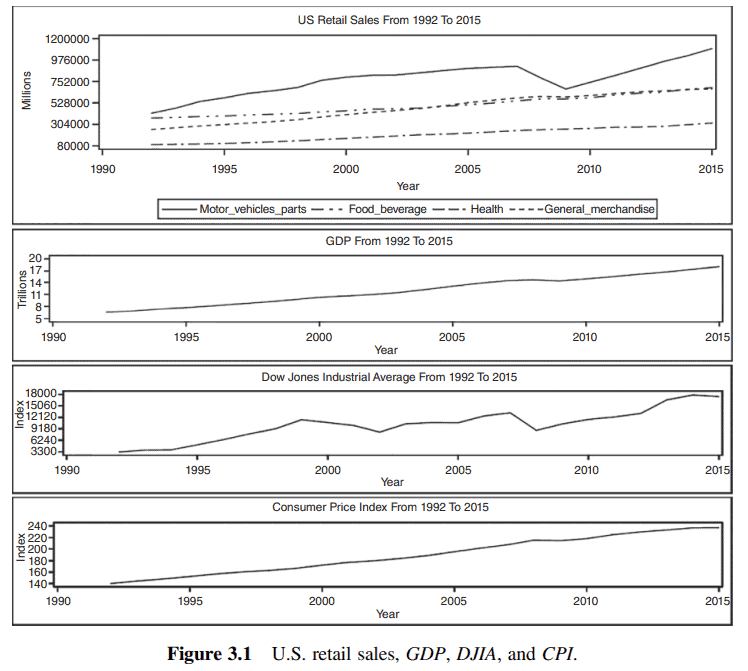
Example 3.1 In this example, we will first examine the OLS regression of U.S. retail sales and some important national indicator variables, including GDP (gross domestic product), DJIA (Dow Jones Industrial Average), and average CPI (consumer price index) from 1992 to 2015. The data set is the WW3a series listed in the Data Appendix and given in Table 3.1 with the plot given in Figure 3.1.
After examining the figure, we will first try the following regression equations

$$
Y_{i, t}=\alpha_i+\beta_{i, 1} G D P_t+\beta_{i, 2} G D P_{t-1}+\beta_{i, 3} G D P_{t-2}+\beta_{i, 4} D J I A_{t-1}+\beta_{i, 5} C P I_t+\xi_{i, t},
$$
where
$Y_{1, t}=$ sales of motor vehicle and parts dealers
$Y_{2, t}=$ sales of food and beverage stores
$Y_{3, t}=$ sales of health care and personal care stores
$Y_{4, t}=$ sales of general merchandise stores
$G D P_t=G D P$ (trillion) at year $t$
$D J I A_{t-1}=$ Dow Jones Industrial Average at beginning of the year
$C P I_t=$ average $C P I$ of the year $(1982-1984=100)$
and the $\xi_{i, t}$ follows independent $N\left(0, \sigma_i^2\right)$. In terms of the OLS regression, Eq. (3.12) becomes

$$
Y_{i, t}=\mathbf{X}t \boldsymbol{\beta}{(i)}+\xi_{i, t},
$$
where
and $\xi_{i, t}$ follows i.i.d.N $\left(0, \sigma_i^2\right)$. The estimation results are given in Table 3.2.

时间序列分析代考

统计代写|时间序列分析代写Time-Series Analysis代考|The Generalized Least Squares (GLS) estimation

如Eq.(3.6)所示，$i$响应$\mathbf{Y}{(i)}$实际上遵循一般的多元时间序列回归模型$$ Y{i, t}=\beta_{i, 0}+\beta_{i, 1} X_{1, t}+\cdots+\beta_{i, k} X_{k, t}+\varepsilon_{i, t}=\mathbf{X}t^{\prime} \boldsymbol{\beta}{(i)}+\xi_{i, t}, t=1, \ldots n
$$
或
$$
\mathbf{Y}{(i)}=\mathbf{X} \boldsymbol{\beta}{(i)}+\boldsymbol{\xi}{(i)} $$其中$\boldsymbol{\xi}{(i)}=\left[\xi_{i, 1}, \xi_{i, 2}, \ldots, \xi_{i, n}\right]^{\prime}$遵循$n$维多元正态分布$N(\mathbf{0}$, $\boldsymbol{\Sigma}{(i)}$)。在时间序列回归中，通常假定$\xi{i, t}$遵循时间序列模型，如$\operatorname{AR}(p)$。从多元回归的结果可知，当$\boldsymbol{\Sigma}{(i)}$已知时，GLS估计量$$ \hat{\boldsymbol{\beta}}{(i)}=\left(\mathbf{X}^{\prime} \mathbf{\Sigma}{(i)}^{-1} \mathbf{X}\right)^{-1} \mathbf{X}^{\prime} \mathbf{\Sigma}{(i)}^{-1} \mathbf{Y}{(i)} $$是最好的无偏估计量。通常，我们不知道$\boldsymbol{\xi}{(i)}$的方差协方差矩阵$\boldsymbol{\Sigma}{(i)}$。即使$\xi{i, t}$遵循时间序列模型(如$\operatorname{AR}(p)$或$\operatorname{ARMA}(p, q)$)，也不知道$\boldsymbol{\Sigma}{(i)}$的结构，因为相关的时间序列模型参数通常是未知的。在这种情况下，我们使用Wei (2006, Chapter 15)建议的以下GLS程序: 步骤1:从(3.8)中模型的OLS拟合中计算普通最小二乘残差$\hat{\xi}{i, t}$。
步骤2:根据OLS残差估计假设时间序列模型的参数$\hat{\xi}{i, t}$步骤3:从步骤2中得到的$\xi_{i, t}$的估计模型中计算$\hat{\boldsymbol{\Sigma}}{(i)}$。
步骤4:使用步骤3中获得的$\hat{\boldsymbol{\Sigma}}_{(i)}$计算GLS估计器$\hat{\boldsymbol{\beta}}{(i)}=\left(\mathbf{X}^{\prime} \hat{\boldsymbol{\Sigma}}{(i)}^{-1} \mathbf{X}\right)^{-1} \mathbf{X}^{\prime} \hat{\mathbf{\Sigma}}{(i)}^{-1} \mathbf{Y}{(i)}$。

统计代写|时间序列分析代写Time-Series Analysis代考|Empirical Example I – U.S. retail sales and some national indicators

在这个例子中，我们将首先检查美国零售销售的OLS回归和一些重要的国家指标变量，包括GDP(国内生产总值)，DJIA(道琼斯工业平均指数)和平均CPI(消费者价格指数)从1992年到2015年。数据集为数据附录中的WW3a系列，见表3.1，图3.1所示。
在检查了图之后，我们将首先尝试下面的回归方程

$$
Y_{i, t}=\alpha_i+\beta_{i, 1} G D P_t+\beta_{i, 2} G D P_{t-1}+\beta_{i, 3} G D P_{t-2}+\beta_{i, 4} D J I A_{t-1}+\beta_{i, 5} C P I_t+\xi_{i, t},
$$
在哪里
$Y_{1, t}=$销售汽车及零部件经销商
$Y_{2, t}=$食品和饮料商店的销售
$Y_{3, t}=$医疗保健和个人护理商店的销售
$Y_{4, t}=$百货商店销售
$G D P_t=G D P$(万亿)在$t$年
$D J I A_{t-1}=$年初道琼斯工业平均指数
$C P I_t=$年平均$C P I$$(1982-1984=100)$
$\xi_{i, t}$跟在独立的$N\left(0, \sigma_i^2\right)$后面。在OLS回归方面，Eq.(3.12)变为

$$
Y_{i, t}=\mathbf{X}t \boldsymbol{\beta}{(i)}+\xi_{i, t},
$$
在哪里
$\xi_{i, t}$跟i.i.d.N $\left(0, \sigma_i^2\right)$。估计结果如表3.2所示。

统计代写请认准statistics-lab™. statistics-lab™为您的留学生涯保驾护航。

金融工程代写

金融工程是使用数学技术来解决金融问题。金融工程使用计算机科学、统计学、经济学和应用数学领域的工具和知识来解决当前的金融问题，以及设计新的和创新的金融产品。

非参数统计代写

非参数统计指的是一种统计方法，其中不假设数据来自于由少数参数决定的规定模型；这种模型的例子包括正态分布模型和线性回归模型。

广义线性模型代考

广义线性模型（GLM）归属统计学领域，是一种应用灵活的线性回归模型。该模型允许因变量的偏差分布有除了正态分布之外的其它分布。

术语 广义线性模型（GLM）通常是指给定连续和/或分类预测因素的连续响应变量的常规线性回归模型。它包括多元线性回归，以及方差分析和方差分析（仅含固定效应）。

有限元方法代写

有限元方法（FEM）是一种流行的方法，用于数值解决工程和数学建模中出现的微分方程。典型的问题领域包括结构分析、传热、流体流动、质量运输和电磁势等传统领域。

有限元是一种通用的数值方法，用于解决两个或三个空间变量的偏微分方程（即一些边界值问题）。为了解决一个问题，有限元将一个大系统细分为更小、更简单的部分，称为有限元。这是通过在空间维度上的特定空间离散化来实现的，它是通过构建对象的网格来实现的：用于求解的数值域，它有有限数量的点。边界值问题的有限元方法表述最终导致一个代数方程组。该方法在域上对未知函数进行逼近。[1] 然后将模拟这些有限元的简单方程组合成一个更大的方程系统，以模拟整个问题。然后，有限元通过变化微积分使相关的误差函数最小化来逼近一个解决方案。

tatistics-lab作为专业的留学生服务机构，多年来已为美国、英国、加拿大、澳洲等留学热门地的学生提供专业的学术服务，包括但不限于Essay代写，Assignment代写，Dissertation代写，Report代写，小组作业代写，Proposal代写，Paper代写，Presentation代写，计算机作业代写，论文修改和润色，网课代做，exam代考等等。写作范围涵盖高中，本科，研究生等海外留学全阶段，辐射金融，经济学，会计学，审计学，管理学等全球99%专业科目。写作团队既有专业英语母语作者，也有海外名校硕博留学生，每位写作老师都拥有过硬的语言能力，专业的学科背景和学术写作经验。我们承诺100%原创，100%专业，100%准时，100%满意。

随机分析代写

随机微积分是数学的一个分支，对随机过程进行操作。它允许为随机过程的积分定义一个关于随机过程的一致的积分理论。这个领域是由日本数学家伊藤清在第二次世界大战期间创建并开始的。

时间序列分析代写

随机过程，是依赖于参数的一组随机变量的全体，参数通常是时间。 随机变量是随机现象的数量表现，其时间序列是一组按照时间发生先后顺序进行排列的数据点序列。通常一组时间序列的时间间隔为一恒定值（如1秒，5分钟，12小时，7天，1年），因此时间序列可以作为离散时间数据进行分析处理。研究时间序列数据的意义在于现实中，往往需要研究某个事物其随时间发展变化的规律。这就需要通过研究该事物过去发展的历史记录，以得到其自身发展的规律。

回归分析代写

多元回归分析渐进（Multiple Regression Analysis Asymptotics）属于计量经济学领域，主要是一种数学上的统计分析方法，可以分析复杂情况下各影响因素的数学关系，在自然科学、社会和经济学等多个领域内应用广泛。

MATLAB代写

MATLAB 是一种用于技术计算的高性能语言。它将计算、可视化和编程集成在一个易于使用的环境中，其中问题和解决方案以熟悉的数学符号表示。典型用途包括：数学和计算算法开发建模、仿真和原型制作数据分析、探索和可视化科学和工程图形应用程序开发，包括图形用户界面构建MATLAB 是一个交互式系统，其基本数据元素是一个不需要维度的数组。这使您可以解决许多技术计算问题，尤其是那些具有矩阵和向量公式的问题，而只需用 C 或 Fortran 等标量非交互式语言编写程序所需的时间的一小部分。MATLAB 名称代表矩阵实验室。MATLAB 最初的编写目的是提供对由 LINPACK 和 EISPACK 项目开发的矩阵软件的轻松访问，这两个项目共同代表了矩阵计算软件的最新技术。MATLAB 经过多年的发展，得到了许多用户的投入。在大学环境中，它是数学、工程和科学入门和高级课程的标准教学工具。在工业领域，MATLAB 是高效研究、开发和分析的首选工具。MATLAB 具有一系列称为工具箱的特定于应用程序的解决方案。对于大多数 MATLAB 用户来说非常重要，工具箱允许您学习和应用专业技术。工具箱是 MATLAB 函数（M 文件）的综合集合，可扩展 MATLAB 环境以解决特定类别的问题。可用工具箱的领域包括信号处理、控制系统、神经网络、模糊逻辑、小波、仿真等。

R语言代写	问卷设计与分析代写
PYTHON代写	回归分析与线性模型代写
MATLAB代写	方差分析与试验设计代写
STATA代写	机器学习/统计学习代写
SPSS代写	计量经济学代写
EVIEWS代写	时间序列分析代写
EXCEL代写	深度学习代写
SQL代写	各种数据建模与可视化代写

如果你也在 怎样代写时间序列分析Time-Series Analysis 这个学科遇到相关的难题，请随时右上角联系我们的24/7代写客服。时间序列分析Time-Series Analysis是在数学中，是按时间顺序索引（或列出或绘制）的一系列数据点。最常见的是，一个时间序列是在连续的等距的时间点上的一个序列。因此，它是一个离散时间数据的序列。时间序列的例子有海洋潮汐的高度、太阳黑子的数量和道琼斯工业平均指数的每日收盘值。

时间序列分析Time-Series Analysis分析包括分析时间序列数据的方法，以提取有意义的统计数据和数据的其他特征。时间序列预测是使用一个模型来预测基于先前观察到的值的未来值。虽然经常采用回归分析的方式来测试一个或多个不同时间序列之间的关系，但这种类型的分析通常不被称为 “时间序列分析”，它特别指的是单一序列中不同时间点之间的关系。中断的时间序列分析是用来检测一个时间序列从之前到之后的演变变化，这种变化可能会影响基础变量。

statistics-lab™ 为您的留学生涯保驾护航 在代写时间序列分析Time-Series Analysis方面已经树立了自己的口碑, 保证靠谱, 高质且原创的统计Statistics代写服务。我们的专家在代写时间序列分析Time-Series Analysis代写方面经验极为丰富，各种代写时间序列分析Time-Series Analysis相关的作业也就用不着说。

统计代写|时间序列分析代写Time-Series Analysis代考|Types of multivariate time series outliers and detections

Suppose we have $m$-dimensional time series $\mathbf{X}t=\left(X{1 t}, X_{2 t}, \ldots, X_{m t}\right)^{\prime}$ that follows a VARMA model
$$
\boldsymbol{\Phi}(B) \mathbf{X}t=\boldsymbol{\Theta}_0+\boldsymbol{\Theta}(B) \mathbf{a}_t $$ where $\mathbf{a}_t=\left(a{1, t}, a_{2, t}, \ldots, a_{m, t}\right)^{\prime}$ is $m$-dimensional Gaussian white noise with mean $\mathbf{0}$ and positivedefinite covariance matrix $\boldsymbol{\Sigma}$. Recall that if $\mathbf{X}_t$ is invertible, the VARMA model in Eq. (2.81) has its corresponding AR representation,
$$
\mathbf{\Pi}(B) \mathbf{X}_t=\mathbf{C}_1+\mathbf{a}_t
$$

where $\boldsymbol{\Pi}(B)={\boldsymbol{\Theta}(B)}^{-1} \boldsymbol{\Phi}(B)$ and $\mathbf{C}1={\boldsymbol{\Theta}(1)}^{-1} \boldsymbol{\Theta}_0$. If $\mathbf{X}_t$ is stationary, we can also have the MA representation, $$ \mathbf{X}_t=\mathrm{C}_2+\Psi(B) \mathbf{a}_t $$ where $\boldsymbol{\Psi}(B)={\boldsymbol{\Phi}(B)}^{-1} \boldsymbol{\Theta}(B)$ and $\mathbf{C}_2={\boldsymbol{\Phi}(1)}^{-1} \boldsymbol{\Theta}_0$. Let $I_t^{(h)}$ be the indicator variable such that $I_h^{(h)}=1$ and $I_t^{(h)}=0$ if $t \neq h$. Suppose we observe time series $\mathbf{Z}_t=\left(Z{1 t}, Z_{2 t}, \ldots, Z_{m t}\right)^{\prime}$, and $\boldsymbol{\omega}=\left(\omega_1, \omega_2, \ldots, \omega_m\right)^{\prime}$ is the size of the outlier. The four types of outlier in univariate time series can be generalized by following formulation
$$
\mathbf{Z}_t=\mathbf{X}_t+\boldsymbol{\alpha}(B) \omega \mathbf{I}_t^{(h)}
$$
The outlier type is defined by the matrix polynomial $\boldsymbol{\alpha}(B)$. Specifically,

• if $\boldsymbol{\alpha}(B)=\boldsymbol{\Psi}(B)$, we have a multivariate innovational outlier (MIO);
• if $\boldsymbol{\alpha}(B)=\mathbf{I}$, we have a multivariate additive outlier (MAO);
• if $\boldsymbol{\alpha}(B)=(1-B)^{-1} \mathbf{I}$, then the outlier is a multivariate level shift (MLS);
• if $\boldsymbol{\alpha}(B)=(\mathbf{I}-\delta \mathbf{I} B)^{-1}$, with a constant $0<\delta<1$, we have a multivariate temporary change (MTC).

统计代写|时间序列分析代写Time-Series Analysis代考|Outlier detection through projection pursuit

Galeano et al. (2006) proposed a method that first projects the MTS into a univariate time series, and then detects outliers within the derived or projected univariate time series. They also suggested an algorithm that finds optimal projection directions by using kurtosis coefficients. This approach has two main advantages. First, it is simple because no multivariate model has to be prespecified. Second, an appropriate projection direction can lead to a test statistic that is more powerful.

To illustrate the method, we use projection of the VARMA model as an example. A linear combination of $m$ multiple time series that follow a VARMA model is a univariate ARMA model. Specifically, let $\mathbf{A}^{\prime}$ be a vector contains the weights of the linear combination and assume $\mathbf{X}_t$ is a $m$-dimensional VARMA $(p, q)$ process. Then, Lütkepohl $(1984,1987)$ showed that $x_t=\mathbf{A}^{\prime} \mathbf{X}_t$ follows a $\operatorname{ARMA}\left(p^, q^\right)$ process with $p^* \leq m p$ and $q^* \leq(m-1) p+q$. Thus, $x_t$ has the following representation
$$
\phi(B) x_t=c+\theta(B) e_t
$$
where $\phi(B)=|\boldsymbol{\Phi}(B)|, c=\mathbf{A}^{\prime} \boldsymbol{\Phi}(1)^* \boldsymbol{\Theta}_0$, and $\mathbf{A}^{\prime} \boldsymbol{\Phi}(B)^* \boldsymbol{\Theta}(B) \mathbf{a}_t=\theta(B) e_t, \boldsymbol{\Phi}(B)^*$ is the adjoint matrix of $\Phi(B)$, and $e_t$ is a univariate white noise process with mean 0 and constant variance $\sigma^2$.
Suppose we observe a time series $\mathbf{Z}_t$ that is affected by an outlier as shown in Eq. (2.84), the projected time series $z_t=\mathbf{A}^{\prime} \mathbf{Z}_t$ can be represented as
$$
z_t=x_t+\mathbf{A}^{\prime} \boldsymbol{\alpha}(B) \boldsymbol{\omega} I_t^{(h)}
$$

时间序列分析代考

of multivariate time series outliers and detections

假设我们有$m$维时间序列$\mathbf{X}t=\left(X{1 t}, X_{2 t}, \ldots, X_{m t}\right)^{\prime}$，它遵循VARMA模型
$$
\boldsymbol{\Phi}(B) \mathbf{X}t=\boldsymbol{\Theta}0+\boldsymbol{\Theta}(B) \mathbf{a}_t $$其中$\mathbf{a}_t=\left(a{1, t}, a{2, t}, \ldots, a_{m, t}\right)^{\prime}$为$m$ -维高斯白噪声，均值为$\mathbf{0}$，正定协方差矩阵为$\boldsymbol{\Sigma}$。回想一下，如果$\mathbf{X}_t$是可逆的，则Eq.(2.81)中的VARMA模型有其对应的AR表示，
$$
\mathbf{\Pi}(B) \mathbf{X}_t=\mathbf{C}_1+\mathbf{a}_t
$$

其中$\boldsymbol{\Pi}(B)={\boldsymbol{\Theta}(B)}^{-1} \boldsymbol{\Phi}(B)$和$\mathbf{C}1={\boldsymbol{\Theta}(1)}^{-1} \boldsymbol{\Theta}0$。如果$\mathbf{X}_t$是平稳的，我们也可以有MA表示，$$ \mathbf{X}_t=\mathrm{C}_2+\Psi(B) \mathbf{a}_t $$其中$\boldsymbol{\Psi}(B)={\boldsymbol{\Phi}(B)}^{-1} \boldsymbol{\Theta}(B)$和$\mathbf{C}_2={\boldsymbol{\Phi}(1)}^{-1} \boldsymbol{\Theta}_0$。让$I_t^{(h)}$作为指示变量，这样$I_h^{(h)}=1$和$I_t^{(h)}=0$如果$t \neq h$。假设我们观察时间序列$\mathbf{Z}_t=\left(Z{1 t}, Z{2 t}, \ldots, Z_{m t}\right)^{\prime}$, $\boldsymbol{\omega}=\left(\omega_1, \omega_2, \ldots, \omega_m\right)^{\prime}$是离群值的大小。单变量时间序列中的四种异常值可以用以下公式进行概括
$$
\mathbf{Z}_t=\mathbf{X}_t+\boldsymbol{\alpha}(B) \omega \mathbf{I}_t^{(h)}
$$
离群值类型由矩阵多项式$\boldsymbol{\alpha}(B)$定义。具体来说，

如果$\boldsymbol{\alpha}(B)=\boldsymbol{\Psi}(B)$，我们有一个多变量创新异常值(MIO);

如果 $\boldsymbol{\alpha}(B)=\mathbf{I}$

如果$\boldsymbol{\alpha}(B)=(1-B)^{-1} \mathbf{I}$，则异常值为多变量水平偏移(MLS);

如果$\boldsymbol{\alpha}(B)=(\mathbf{I}-\delta \mathbf{I} B)^{-1}$加上常数$0<\delta<1$，我们就得到了一个多变量临时变化(MTC)。

统计代写|时间序列分析代写Time-Series Analysis代考|Outlier detection through projection pursuit

Galeano et al.(2006)提出了一种方法，该方法首先将MTS投影到单变量时间序列中，然后在导出或投影的单变量时间序列中检测异常值。他们还提出了一种利用峰度系数找到最佳投影方向的算法。这种方法有两个主要优点。首先，它很简单，因为不需要预先指定多变量模型。其次，适当的投影方向可以产生更强大的测试统计量。

为了说明该方法，我们以VARMA模型的投影为例。遵循VARMA模型的$m$多个时间序列的线性组合是单变量ARMA模型。具体地说，设$\mathbf{A}^{\prime}$是一个包含线性组合权重的向量，并假设$\mathbf{X}_t$是一个$m$维VARMA $(p, q)$过程。然后，l tkepohl $(1984,1987)$表明$x_t=\mathbf{A}^{\prime} \mathbf{X}_t$遵循$p^* \leq m p$和$q^* \leq(m-1) p+q$的$\operatorname{ARMA}\left(p^, q^\right)$过程。因此，$x_t$具有以下表示形式
$$
\phi(B) x_t=c+\theta(B) e_t
$$
式中$\phi(B)=|\boldsymbol{\Phi}(B)|, c=\mathbf{A}^{\prime} \boldsymbol{\Phi}(1)^* \boldsymbol{\Theta}_0$, $\mathbf{A}^{\prime} \boldsymbol{\Phi}(B)^* \boldsymbol{\Theta}(B) \mathbf{a}_t=\theta(B) e_t, \boldsymbol{\Phi}(B)^*$为$\Phi(B)$的伴随矩阵，$e_t$为均值为0，方差为常数的单变量白噪声过程$\sigma^2$。
假设我们观察到一个受异常值影响的时间序列$\mathbf{Z}_t$，如式(2.84)所示，那么预测的时间序列$z_t=\mathbf{A}^{\prime} \mathbf{Z}_t$可以表示为
$$
z_t=x_t+\mathbf{A}^{\prime} \boldsymbol{\alpha}(B) \boldsymbol{\omega} I_t^{(h)}
$$

统计代写请认准statistics-lab™. statistics-lab™为您的留学生涯保驾护航。

金融工程代写

金融工程是使用数学技术来解决金融问题。金融工程使用计算机科学、统计学、经济学和应用数学领域的工具和知识来解决当前的金融问题，以及设计新的和创新的金融产品。

非参数统计代写

非参数统计指的是一种统计方法，其中不假设数据来自于由少数参数决定的规定模型；这种模型的例子包括正态分布模型和线性回归模型。

广义线性模型代考

广义线性模型（GLM）归属统计学领域，是一种应用灵活的线性回归模型。该模型允许因变量的偏差分布有除了正态分布之外的其它分布。

术语 广义线性模型（GLM）通常是指给定连续和/或分类预测因素的连续响应变量的常规线性回归模型。它包括多元线性回归，以及方差分析和方差分析（仅含固定效应）。

有限元方法代写

有限元方法（FEM）是一种流行的方法，用于数值解决工程和数学建模中出现的微分方程。典型的问题领域包括结构分析、传热、流体流动、质量运输和电磁势等传统领域。

有限元是一种通用的数值方法，用于解决两个或三个空间变量的偏微分方程（即一些边界值问题）。为了解决一个问题，有限元将一个大系统细分为更小、更简单的部分，称为有限元。这是通过在空间维度上的特定空间离散化来实现的，它是通过构建对象的网格来实现的：用于求解的数值域，它有有限数量的点。边界值问题的有限元方法表述最终导致一个代数方程组。该方法在域上对未知函数进行逼近。[1] 然后将模拟这些有限元的简单方程组合成一个更大的方程系统，以模拟整个问题。然后，有限元通过变化微积分使相关的误差函数最小化来逼近一个解决方案。

tatistics-lab作为专业的留学生服务机构，多年来已为美国、英国、加拿大、澳洲等留学热门地的学生提供专业的学术服务，包括但不限于Essay代写，Assignment代写，Dissertation代写，Report代写，小组作业代写，Proposal代写，Paper代写，Presentation代写，计算机作业代写，论文修改和润色，网课代做，exam代考等等。写作范围涵盖高中，本科，研究生等海外留学全阶段，辐射金融，经济学，会计学，审计学，管理学等全球99%专业科目。写作团队既有专业英语母语作者，也有海外名校硕博留学生，每位写作老师都拥有过硬的语言能力，专业的学科背景和学术写作经验。我们承诺100%原创，100%专业，100%准时，100%满意。

随机分析代写

随机微积分是数学的一个分支，对随机过程进行操作。它允许为随机过程的积分定义一个关于随机过程的一致的积分理论。这个领域是由日本数学家伊藤清在第二次世界大战期间创建并开始的。

时间序列分析代写

随机过程，是依赖于参数的一组随机变量的全体，参数通常是时间。 随机变量是随机现象的数量表现，其时间序列是一组按照时间发生先后顺序进行排列的数据点序列。通常一组时间序列的时间间隔为一恒定值（如1秒，5分钟，12小时，7天，1年），因此时间序列可以作为离散时间数据进行分析处理。研究时间序列数据的意义在于现实中，往往需要研究某个事物其随时间发展变化的规律。这就需要通过研究该事物过去发展的历史记录，以得到其自身发展的规律。

回归分析代写

多元回归分析渐进（Multiple Regression Analysis Asymptotics）属于计量经济学领域，主要是一种数学上的统计分析方法，可以分析复杂情况下各影响因素的数学关系，在自然科学、社会和经济学等多个领域内应用广泛。

MATLAB代写

MATLAB 是一种用于技术计算的高性能语言。它将计算、可视化和编程集成在一个易于使用的环境中，其中问题和解决方案以熟悉的数学符号表示。典型用途包括：数学和计算算法开发建模、仿真和原型制作数据分析、探索和可视化科学和工程图形应用程序开发，包括图形用户界面构建MATLAB 是一个交互式系统，其基本数据元素是一个不需要维度的数组。这使您可以解决许多技术计算问题，尤其是那些具有矩阵和向量公式的问题，而只需用 C 或 Fortran 等标量非交互式语言编写程序所需的时间的一小部分。MATLAB 名称代表矩阵实验室。MATLAB 最初的编写目的是提供对由 LINPACK 和 EISPACK 项目开发的矩阵软件的轻松访问，这两个项目共同代表了矩阵计算软件的最新技术。MATLAB 经过多年的发展，得到了许多用户的投入。在大学环境中，它是数学、工程和科学入门和高级课程的标准教学工具。在工业领域，MATLAB 是高效研究、开发和分析的首选工具。MATLAB 具有一系列称为工具箱的特定于应用程序的解决方案。对于大多数 MATLAB 用户来说非常重要，工具箱允许您学习和应用专业技术。工具箱是 MATLAB 函数（M 文件）的综合集合，可扩展 MATLAB 环境以解决特定类别的问题。可用工具箱的领域包括信号处理、控制系统、神经网络、模糊逻辑、小波、仿真等。

R语言代写	问卷设计与分析代写
PYTHON代写	回归分析与线性模型代写
MATLAB代写	方差分析与试验设计代写
STATA代写	机器学习/统计学习代写
SPSS代写	计量经济学代写
EVIEWS代写	时间序列分析代写
EXCEL代写	深度学习代写
SQL代写	各种数据建模与可视化代写

如果你也在 怎样代写时间序列分析Time-Series Analysis这个学科遇到相关的难题，请随时右上角联系我们的24/7代写客服。

时间序列分析是分析在一个时间间隔内收集的一系列数据点的具体方式。在时间序列分析中，分析人员在设定的时间段内以一致的时间间隔记录数据点，而不仅仅是间歇性或随机地记录数据点。

statistics-lab™ 为您的留学生涯保驾护航 在代写时间序列分析Time-Series Analysis方面已经树立了自己的口碑, 保证靠谱, 高质且原创的统计Statistics代写服务。我们的专家在代写时间序列分析Time-Series Analysis代写方面经验极为丰富，各种代写时间序列分析Time-Series Analysis相关的作业也就用不着说。

我们提供的时间序列分析Time-Series Analysis及其相关学科的代写，服务范围广, 其中包括但不限于:

• Statistical Inference 统计推断
• Statistical Computing 统计计算
• Advanced Probability Theory 高等概率论
• Advanced Mathematical Statistics 高等数理统计学
• (Generalized) Linear Models 广义线性模型
• Statistical Machine Learning 统计机器学习
• Longitudinal Data Analysis 纵向数据分析
• Foundations of Data Science 数据科学基础

统计代写|时间序列分析代写Time-Series Analysis代考|Identification of vector time series models

In constructing a vector time series model, just like in univariate time series model building, the first step is to plot the vector time series. By plotting all the component series in one graph, we obtain a good idea of the movements of different components and the general pattern of their relationships. In principle, the vector time series model building procedure is similar to the univariate time series model building procedure. We identify an underlying model from its correlation and partial correlation matrix functions. Table 2.1 gives a useful summary.

Given an observed vector time series $\mathbf{Z}_1, \ldots, \mathbf{Z}_n$, we compute its sample correlation and partial correlation matrices after proper transformations are applied to reduce a nonstationary series to a stationary series.

For a stationary $m$-dimensional vector time series process, given the $n$ observations, $\mathbf{Z}1, \ldots, \mathbf{Z}_n$, the mean vector, $\boldsymbol{\mu}$, is estimated by its sample mean vector, $$ \overline{\mathbf{Z}}=\frac{1}{n} \sum{t=1}^n \mathbf{Z}t=\frac{1}{n}\left[\begin{array}{c} \sum{t=1}^n Z_{1, t} \
\sum_{t=1}^n Z_{2, t} \
\vdots \
\sum_{t=1}^n Z_{m, t}
\end{array}\right]=\left[\begin{array}{c}
\bar{Z}1 \ \bar{Z}_2 \ \vdots \ \bar{Z}_m \end{array}\right] . $$ It can be easily seen that $E(\overline{\mathbf{Z}})=\boldsymbol{\mu}$, and $\overline{\mathbf{Z}}$ is an unbiased estimator of $\boldsymbol{\mu}$. Since $$ E(\overline{\mathbf{Z}}-\boldsymbol{\mu})(\overline{\mathbf{Z}}-\boldsymbol{\mu})^{\prime}=\frac{1}{n^2} \sum{i=1}^n \sum_{j=1}^n \boldsymbol{\Gamma}(i-j)=\frac{1}{n} \sum_{k=-(n-1)}^{n-1}\left(1-\frac{k}{n}\right) \boldsymbol{\Gamma}(k)
$$
for a stationary vector process with $\rho_{i, i}(k) \rightarrow 0$ as $k \rightarrow 0, \overline{\mathbf{Z}}$ is actually a consistent estimator of $\boldsymbol{\mu}$. So,
$$
E(\overline{\mathbf{Z}}-\boldsymbol{\mu})(\overline{\mathbf{Z}}-\boldsymbol{\mu})^{\prime} \rightarrow 0 \text { as } n \rightarrow \infty
$$
and
$$
\lim {n \rightarrow \infty}\left{n E\left[(\overline{\mathbf{Z}}-\boldsymbol{\mu})(\overline{\mathbf{Z}}-\boldsymbol{\mu})^{\prime}\right]\right}=\sum{k=-\infty}^{\infty} \boldsymbol{\Gamma}(k)
$$

统计代写|时间序列分析代写Time-Series Analysis代考|Sample correlation matrix function

The correlation matrix function, $\boldsymbol{\rho}(k)=\left[\rho_{i, j}(k)\right]$ is estimated by the sample correlation matrix function given by
$$
\hat{\boldsymbol{\rho}}(k)=\left[\hat{\rho}{i, j}(k)\right] $$ where the $\hat{\rho}{i, j}(k)$ represents the sample cross-correlations between the $i$ th and $j$ th component series at lag $k$, that is,
$$
\hat{\rho}{i, j}(k)=\frac{\hat{\gamma}{i, j}(k)}{\left[\hat{\gamma}{i, i}(0)\right]^{1 / 2}\left[\hat{\gamma}{j, j}(0)\right]^{1 / 2}}=\frac{\sum_{t=1}^{n-k}\left(Z_{i, t}-\bar{Z}i\right)\left(Z{j, t+k}-\bar{Z}j\right)}{\left[\sum{t=1}^n\left(Z_{i, t}-\bar{Z}i\right)^2 \sum{t=1}^n\left(Z_{j, t}-\bar{Z}j\right)^2\right]^{1 / 2}} . $$ Although $\hat{\boldsymbol{\Gamma}}(k)$ and $\hat{\boldsymbol{\rho}}(k)$ are not unbiased estimators of $\boldsymbol{\Gamma}(k)$ and $\boldsymbol{\rho}(k)$ for a stationary vector process, they are consistent estimators, and the $\hat{\rho}{i, j}(k)$ are asymptotically normally distributed with means $\rho_{i, j}(k)$ and the variance given by Bartlett (1955) shown next
$$
\operatorname{Var}\left[\hat{\rho}{i, j}(k)\right] \approx \frac{1}{n-k} \sum{h=-\infty}^{\infty}\left{\begin{array}{l}
\rho_{i, i}(h) \rho_{j, j}(h)+\rho_{i, j}(k+h) \rho_{i, j}(k-h) \
+\rho_{i, j}^2(k)\left[\rho_{i, j}^2(h)+\frac{1}{2} \rho_{i, i}^2(h)+\frac{1}{2} \rho_{j, j}^2(h)\right] \
-2 \rho_{i, j}(k)\left[\rho_{i, i}(h) \rho_{i, j}(h+k)+\rho_{j, j}(h) \rho_{i, j}(h-k)\right]
\end{array}\right} .
$$

If $\rho_{i, j}(k)=0$ for $|k|>q$ for some $q$, then
$$
\operatorname{Var}\left[\hat{\rho}{i, j}(k)\right] \approx \frac{1}{n-k}\left[1+2 \sum{h=1}^q\left{\rho_{i, i}(h) \rho_{j, j}(h)\right}, \text { for }|k|>q\right.
$$
When the $\mathbf{Z}t$ series are vector white noise, we have $$ \operatorname{Var}\left[\hat{\rho}{i, j}(k)\right] \approx \frac{1}{n-k}
$$
For large samples, $(n-k)$ is often replaced by $n$ in these expressions. The other related reference is Hannan (1970, p. 228).

时间序列分析代考

统计代写|时间序列分析代写Time-Series Analysis代考|Identification of vector time series models

在构建向量时间序列模型时，与构建单变量时间序列模型一样，第一步是绘制向量时间序列。通过在一个图中绘制所有的分量序列，我们可以很好地了解不同分量的运动和它们之间关系的一般模式。原则上，向量时间序列模型的建立过程与单变量时间序列模型的建立过程类似。我们从相关矩阵和偏相关矩阵函数中识别出一个潜在的模型。表2.1给出了一个有用的总结。

给定一个观测到的向量时间序列$\mathbf{Z}_1, \ldots, \mathbf{Z}_n$，在应用适当的变换将非平稳序列简化为平稳序列后，我们计算其样本相关矩阵和偏相关矩阵。

对于一个平稳的$m$维向量时间序列过程，给定$n$观测值，$\mathbf{Z}1, \ldots, \mathbf{Z}n$，均值向量$\boldsymbol{\mu}$由其样本均值向量$$ \overline{\mathbf{Z}}=\frac{1}{n} \sum{t=1}^n \mathbf{Z}t=\frac{1}{n}\left[\begin{array}{c} \sum{t=1}^n Z{1, t} \
\sum_{t=1}^n Z_{2, t} \
\vdots \
\sum_{t=1}^n Z_{m, t}
\end{array}\right]=\left[\begin{array}{c}
\bar{Z}1 \ \bar{Z}2 \ \vdots \ \bar{Z}_m \end{array}\right] . $$估计，可以很容易地看出$E(\overline{\mathbf{Z}})=\boldsymbol{\mu}$, $\overline{\mathbf{Z}}$是$\boldsymbol{\mu}$的无偏估计量。从$$ E(\overline{\mathbf{Z}}-\boldsymbol{\mu})(\overline{\mathbf{Z}}-\boldsymbol{\mu})^{\prime}=\frac{1}{n^2} \sum{i=1}^n \sum{j=1}^n \boldsymbol{\Gamma}(i-j)=\frac{1}{n} \sum_{k=-(n-1)}^{n-1}\left(1-\frac{k}{n}\right) \boldsymbol{\Gamma}(k)
$$开始
对于一个平稳矢量过程，$\rho_{i, i}(k) \rightarrow 0$作为$k \rightarrow 0, \overline{\mathbf{Z}}$实际上是$\boldsymbol{\mu}$的一致估计量。所以，
$$
E(\overline{\mathbf{Z}}-\boldsymbol{\mu})(\overline{\mathbf{Z}}-\boldsymbol{\mu})^{\prime} \rightarrow 0 \text { as } n \rightarrow \infty
$$
和
$$
\lim {n \rightarrow \infty}\left{n E\left[(\overline{\mathbf{Z}}-\boldsymbol{\mu})(\overline{\mathbf{Z}}-\boldsymbol{\mu})^{\prime}\right]\right}=\sum{k=-\infty}^{\infty} \boldsymbol{\Gamma}(k)
$$

统计代写|时间序列分析代写Time-Series Analysis代考|Sample correlation matrix function

相关矩阵函数$\boldsymbol{\rho}(k)=\left[\rho_{i, j}(k)\right]$由给出的样本相关矩阵函数估计
$$
\hat{\boldsymbol{\rho}}(k)=\left[\hat{\rho}{i, j}(k)\right] $$其中$\hat{\rho}{i, j}(k)$表示$i$ th和$j$ th分量序列滞后$k$时的样本相互关系，即:
$$
\hat{\rho}{i, j}(k)=\frac{\hat{\gamma}{i, j}(k)}{\left[\hat{\gamma}{i, i}(0)\right]^{1 / 2}\left[\hat{\gamma}{j, j}(0)\right]^{1 / 2}}=\frac{\sum_{t=1}^{n-k}\left(Z_{i, t}-\bar{Z}i\right)\left(Z{j, t+k}-\bar{Z}j\right)}{\left[\sum{t=1}^n\left(Z_{i, t}-\bar{Z}i\right)^2 \sum{t=1}^n\left(Z_{j, t}-\bar{Z}j\right)^2\right]^{1 / 2}} . $$虽然$\hat{\boldsymbol{\Gamma}}(k)$和$\hat{\boldsymbol{\rho}}(k)$不是平稳矢量过程的$\boldsymbol{\Gamma}(k)$和$\boldsymbol{\rho}(k)$的无偏估计量，但它们是一致估计量，并且$\hat{\rho}{i, j}(k)$是渐近正态分布，其均值为$\rho_{i, j}(k)$，方差由Bartlett(1955)给出，如下所示
$$
\operatorname{Var}\left[\hat{\rho}{i, j}(k)\right] \approx \frac{1}{n-k} \sum{h=-\infty}^{\infty}\left{\begin{array}{l}
\rho_{i, i}(h) \rho_{j, j}(h)+\rho_{i, j}(k+h) \rho_{i, j}(k-h) \
+\rho_{i, j}^2(k)\left[\rho_{i, j}^2(h)+\frac{1}{2} \rho_{i, i}^2(h)+\frac{1}{2} \rho_{j, j}^2(h)\right] \
-2 \rho_{i, j}(k)\left[\rho_{i, i}(h) \rho_{i, j}(h+k)+\rho_{j, j}(h) \rho_{i, j}(h-k)\right]
\end{array}\right} .
$$

如果$\rho_{i, j}(k)=0$ = $|k|>q$ = $q$，那么
$$
\operatorname{Var}\left[\hat{\rho}{i, j}(k)\right] \approx \frac{1}{n-k}\left[1+2 \sum{h=1}^q\left{\rho_{i, i}(h) \rho_{j, j}(h)\right}, \text { for }|k|>q\right.
$$
当$\mathbf{Z}t$级数是矢量白噪声时，我们得到$$ \operatorname{Var}\left[\hat{\rho}{i, j}(k)\right] \approx \frac{1}{n-k}
$$
对于大样本，在这些表达式中$(n-k)$通常被$n$代替。另一个相关的参考文献是Hannan (1970, p. 228)。

统计代写请认准statistics-lab™. statistics-lab™为您的留学生涯保驾护航。

金融工程代写

金融工程是使用数学技术来解决金融问题。金融工程使用计算机科学、统计学、经济学和应用数学领域的工具和知识来解决当前的金融问题，以及设计新的和创新的金融产品。

非参数统计代写

非参数统计指的是一种统计方法，其中不假设数据来自于由少数参数决定的规定模型；这种模型的例子包括正态分布模型和线性回归模型。

广义线性模型代考

广义线性模型（GLM）归属统计学领域，是一种应用灵活的线性回归模型。该模型允许因变量的偏差分布有除了正态分布之外的其它分布。

术语 广义线性模型（GLM）通常是指给定连续和/或分类预测因素的连续响应变量的常规线性回归模型。它包括多元线性回归，以及方差分析和方差分析（仅含固定效应）。

有限元方法代写

有限元方法（FEM）是一种流行的方法，用于数值解决工程和数学建模中出现的微分方程。典型的问题领域包括结构分析、传热、流体流动、质量运输和电磁势等传统领域。

有限元是一种通用的数值方法，用于解决两个或三个空间变量的偏微分方程（即一些边界值问题）。为了解决一个问题，有限元将一个大系统细分为更小、更简单的部分，称为有限元。这是通过在空间维度上的特定空间离散化来实现的，它是通过构建对象的网格来实现的：用于求解的数值域，它有有限数量的点。边界值问题的有限元方法表述最终导致一个代数方程组。该方法在域上对未知函数进行逼近。[1] 然后将模拟这些有限元的简单方程组合成一个更大的方程系统，以模拟整个问题。然后，有限元通过变化微积分使相关的误差函数最小化来逼近一个解决方案。

tatistics-lab作为专业的留学生服务机构，多年来已为美国、英国、加拿大、澳洲等留学热门地的学生提供专业的学术服务，包括但不限于Essay代写，Assignment代写，Dissertation代写，Report代写，小组作业代写，Proposal代写，Paper代写，Presentation代写，计算机作业代写，论文修改和润色，网课代做，exam代考等等。写作范围涵盖高中，本科，研究生等海外留学全阶段，辐射金融，经济学，会计学，审计学，管理学等全球99%专业科目。写作团队既有专业英语母语作者，也有海外名校硕博留学生，每位写作老师都拥有过硬的语言能力，专业的学科背景和学术写作经验。我们承诺100%原创，100%专业，100%准时，100%满意。

随机分析代写

随机微积分是数学的一个分支，对随机过程进行操作。它允许为随机过程的积分定义一个关于随机过程的一致的积分理论。这个领域是由日本数学家伊藤清在第二次世界大战期间创建并开始的。

时间序列分析代写

随机过程，是依赖于参数的一组随机变量的全体，参数通常是时间。 随机变量是随机现象的数量表现，其时间序列是一组按照时间发生先后顺序进行排列的数据点序列。通常一组时间序列的时间间隔为一恒定值（如1秒，5分钟，12小时，7天，1年），因此时间序列可以作为离散时间数据进行分析处理。研究时间序列数据的意义在于现实中，往往需要研究某个事物其随时间发展变化的规律。这就需要通过研究该事物过去发展的历史记录，以得到其自身发展的规律。

回归分析代写

多元回归分析渐进（Multiple Regression Analysis Asymptotics）属于计量经济学领域，主要是一种数学上的统计分析方法，可以分析复杂情况下各影响因素的数学关系，在自然科学、社会和经济学等多个领域内应用广泛。

MATLAB代写

MATLAB 是一种用于技术计算的高性能语言。它将计算、可视化和编程集成在一个易于使用的环境中，其中问题和解决方案以熟悉的数学符号表示。典型用途包括：数学和计算算法开发建模、仿真和原型制作数据分析、探索和可视化科学和工程图形应用程序开发，包括图形用户界面构建MATLAB 是一个交互式系统，其基本数据元素是一个不需要维度的数组。这使您可以解决许多技术计算问题，尤其是那些具有矩阵和向量公式的问题，而只需用 C 或 Fortran 等标量非交互式语言编写程序所需的时间的一小部分。MATLAB 名称代表矩阵实验室。MATLAB 最初的编写目的是提供对由 LINPACK 和 EISPACK 项目开发的矩阵软件的轻松访问，这两个项目共同代表了矩阵计算软件的最新技术。MATLAB 经过多年的发展，得到了许多用户的投入。在大学环境中，它是数学、工程和科学入门和高级课程的标准教学工具。在工业领域，MATLAB 是高效研究、开发和分析的首选工具。MATLAB 具有一系列称为工具箱的特定于应用程序的解决方案。对于大多数 MATLAB 用户来说非常重要，工具箱允许您学习和应用专业技术。工具箱是 MATLAB 函数（M 文件）的综合集合，可扩展 MATLAB 环境以解决特定类别的问题。可用工具箱的领域包括信号处理、控制系统、神经网络、模糊逻辑、小波、仿真等。

R语言代写	问卷设计与分析代写
PYTHON代写	回归分析与线性模型代写
MATLAB代写	方差分析与试验设计代写
STATA代写	机器学习/统计学习代写
SPSS代写	计量经济学代写
EVIEWS代写	时间序列分析代写
EXCEL代写	深度学习代写
SQL代写	各种数据建模与可视化代写

如果你也在 怎样代写时间序列分析Time-Series Analysis这个学科遇到相关的难题，请随时右上角联系我们的24/7代写客服。

时间序列分析是分析在一个时间间隔内收集的一系列数据点的具体方式。在时间序列分析中，分析人员在设定的时间段内以一致的时间间隔记录数据点，而不仅仅是间歇性或随机地记录数据点。

statistics-lab™ 为您的留学生涯保驾护航 在代写时间序列分析Time-Series Analysis方面已经树立了自己的口碑, 保证靠谱, 高质且原创的统计Statistics代写服务。我们的专家在代写时间序列分析Time-Series Analysis代写方面经验极为丰富，各种代写时间序列分析Time-Series Analysis相关的作业也就用不着说。

我们提供的时间序列分析Time-Series Analysis及其相关学科的代写，服务范围广, 其中包括但不限于:

• Statistical Inference 统计推断
• Statistical Computing 统计计算
• Advanced Probability Theory 高等概率论
• Advanced Mathematical Statistics 高等数理统计学
• (Generalized) Linear Models 广义线性模型
• Statistical Machine Learning 统计机器学习
• Longitudinal Data Analysis 纵向数据分析
• Foundations of Data Science 数据科学基础

统计代写|时间序列分析代写Time-Series Analysis代考|Multivariate Portmanteau Test

As in univariate case, it is critical both to check if a $K$-dimensional stationary vector time series $\mathbf{X}_t$ is correlated and test whether a resulting residual series is a white noise series. The portmanteau test for univariate time series has been extended to the vector case by several authors, for example, Hosking (1980), Li and McLeod (1981). And up to now, the topic has still been under investigation, seeing, for instance, Mahdi and Mcleod (2012) and Thu (2017).

Suppose that the sample $\mathbf{X}{1: T}=\left{\mathbf{X}_1, \mathbf{X}_2, \cdots, \mathbf{X}_T\right}$ of size $T$ comes from a stationary $K$-dimensional time series $\mathbf{X}_t$ with mean vector $\mathbf{0}$ and covariance matrix $\boldsymbol{\Sigma}=\boldsymbol{\Gamma}(0)$. Evidently, $\mathbf{X}_t$ is a white noise series if and only if $\rho(h)=\mathbf{0}$ for any integer $h>0$. The multivariate portmanteau test is designed for testing $H_0: \rho(1)=$ $\rho(2)=\cdots=\rho(m)=\mathbf{0}$ versus $H_1: \rho(s) \neq \mathbf{0}$ for some $1 \leq s \leq m$ where $m$ is a positive integer. The original test statistic is $$ Q(m)=T \sum{h=1}^m \operatorname{tr}\left[\hat{\boldsymbol{\Gamma}}(h)^{\prime} \hat{\boldsymbol{\Gamma}}(0)^{-1} \hat{\boldsymbol{\Gamma}}(h) \hat{\boldsymbol{\Gamma}}(0)^{-1}\right]
$$

There are two widely used modifications of (7.4). One is
$$
Q_{L B}(m)=T^2 \sum_{h=1}^m \frac{1}{T-h} \operatorname{tr}\left[\hat{\boldsymbol{\Gamma}}(h)^{\prime} \hat{\boldsymbol{\Gamma}}(0)^{-1} \hat{\boldsymbol{\Gamma}}(h) \hat{\boldsymbol{\Gamma}}(0)^{-1}\right]
$$
which is similar to the Ljung-Box test statistic in the univariate case and often known as the multivariate Ljung-Box test statistic and introduced by Hosking (1980). The other is
$$
Q_{L M}(m)=T \sum_{h=1}^m \operatorname{tr}\left[\hat{\boldsymbol{\Gamma}}(h)^{\prime} \hat{\boldsymbol{\Gamma}}(0)^{-1} \hat{\boldsymbol{\Gamma}}(h) \hat{\boldsymbol{\Gamma}}(0)^{-1}\right]+\frac{K^2 m(m+1)}{2 T}
$$
which is given by Li and McLeod (1981). In general, both (7.5) and (7.6) provide considerable improvements over (7.4). See, for example, Lütkepohl (2005) and $\mathrm{Li}$ (2004). On the other hand, in the large-sample case, both $Q_{L B}(m)$ and $Q_{L M}(m)$ are asymptotically equivalent to $Q(m)$. And under the null hypothesis and certain other mild conditions, the three portmanteau statistics all are asymptotically chi-squared distributed with degrees of freedom $m K^2$.

统计代写|时间序列分析代写Time-Series Analysis代考|VARMA Models

Definition 7.5 (1) Suppose that $p, q$ are both nonnegative integers, and then the following equation is called the $K$-dimensional vector (multivariate) autoregressive moving average model of order $(p, q)$ and denoted by $\operatorname{VARMA}(p, q)$ :
$$
\mathbf{X}t-\boldsymbol{\Phi}_1 \mathbf{X}{t-1}-\cdots-\boldsymbol{\Phi}p \mathbf{X}{t-p}=\boldsymbol{v}+\boldsymbol{\varepsilon}t+\boldsymbol{\Theta}_1 \boldsymbol{\varepsilon}{t-1}+\cdots+\boldsymbol{\Theta}q \boldsymbol{\varepsilon}{t-q}
$$
where $\boldsymbol{v}$ is a $K$-dimensional constant vector; $\boldsymbol{\varepsilon}_t \sim \operatorname{WN}(\boldsymbol{0}, \boldsymbol{\Sigma})$; $\boldsymbol{\Phi}_1, \cdots, \boldsymbol{\Phi}_p$ are AR part $K \times K$ matrix parameters (coefficients) with $\boldsymbol{\Phi}_p \neq \mathbf{0} ; \boldsymbol{\Theta}_1, \cdots, \boldsymbol{\Theta}_q$ are MA part $K \times K$ matrix parameters (coefficients) with $\boldsymbol{\Theta}_q \neq \mathbf{0}$. (2) If a vector time series $\left{\mathbf{X}_t\right}$ is stationary and satisfies such an equation as (7.7), then we call it a $\operatorname{VARMA}(p, q)$ process.
We give some remarks on Definition 7.5:

• If the vector time series $\left{\mathbf{X}_t\right}$ is a $\operatorname{VARMA}(p, q)$ process or $\operatorname{VARMA}(p, q)$ model (7.7) is stationary, then its mean vector
  $$
  \boldsymbol{\mu}=\mathrm{E}\left(\mathbf{X}_t\right)=\left(I-\boldsymbol{\Phi}_1-\cdots-\boldsymbol{\Phi}_p\right)^{-1} \boldsymbol{v}
  $$
  where $I$ is an identity matrix.
• Using the backshift (lag) operator $B$, the $\operatorname{VARMA}(p, q)$ model can be rewritten as
  $$
  \boldsymbol{\Phi}(B) \mathbf{X}_t=\boldsymbol{v}+\boldsymbol{\Theta}(B) \varepsilon_t
  $$
  where $\boldsymbol{\Phi}(z)=I_K-\boldsymbol{\Phi}_1 z-\cdots-\boldsymbol{\Phi}_p z^p$ and $\boldsymbol{\Theta}(z)=I_K+\boldsymbol{\Theta}_1 z+\cdots+\boldsymbol{\Theta}_q z^q$ are, respectively, VAR and VMA matrix polynomials. Note that each element of the matrices $\boldsymbol{\Phi}(z), \boldsymbol{\Theta}(z)$ is a polynomial with real coefficients and degree less than or equal to $p, q$, respectively.
• If $p>0, q=0$, then the $\operatorname{VARMA}(p, q)$ model reduces to the $\operatorname{VAR}(p)$ model
  $$
  \mathbf{X}t=\boldsymbol{v}+\boldsymbol{\Phi}_1 \mathbf{X}{t-1}+\cdots+\boldsymbol{\Phi}p \mathbf{X}{t-p}+\boldsymbol{\varepsilon}_t \text {, namely } \boldsymbol{\Phi}(B) \mathbf{X}_t=\boldsymbol{v}+\boldsymbol{\varepsilon}_t .
  $$
  This is an extremely useful subclass of VARMA models and is also called the VAR part of VARMA model (7.7).
• If $p=0, q>0$, then the $\operatorname{VARMA}(p, q)$ model reduces to the $\operatorname{VMA}(q)$ model
  $$
  \mathbf{X}t=\boldsymbol{v}+\boldsymbol{\varepsilon}_t+\boldsymbol{\Theta}_1 \varepsilon{t-1}+\cdots+\boldsymbol{\Theta}q \varepsilon{t-q} \text {, namely } \mathbf{X}_t=\boldsymbol{v}+\boldsymbol{\Theta}(B) \boldsymbol{\varepsilon}_t .
  $$
  It is also known as the VMA part of VARMA model (7.7).

时间序列分析代考

统计代写|时间序列分析代写Time-Series Analysis代考|Multivariate Portmanteau Test

与单变量情况一样，检查是否 $K$ 维平稳向量时间序列 $\mathbf{X}t$ 相关并测试生成的残差序列是否为白噪声序列。 多位作者已将单变量时间序列的组合检验扩展到向量情况，例如 Hosking (1980)、Li 和 McLeod (1981)。到目前为止，该主题仍在调查中，例如 Mahdi 和 Mcleod (2012) 以及 Thu (2017)。 的 $K$ 维时间序列 $\mathbf{X}_t$ 均值向量 0 和协方差矩阵 $\boldsymbol{\Sigma}=\boldsymbol{\Gamma}(0)$. 显然， $\mathbf{X}_t$ 是白橾声序列当且仅当 $\rho(h)=\mathbf{0}$ 对 于任何整数 $h>0$. 多变量混成词测试专为测试而设计 $H_0: \rho(1)=\rho(2)=\cdots=\rho(m)=\mathbf{0}$ 相对 $H_1: \rho(s) \neq \mathbf{0}$ 对于一些 $1 \leq s \leq m$ 在哪里 $m$ 是一个正整数。原始检验统计量为 $$ Q(m)=T \sum h=1^m \operatorname{tr}\left[\hat{\boldsymbol{\Gamma}}(h)^{\prime} \hat{\boldsymbol{\Gamma}}(0)^{-1} \hat{\boldsymbol{\Gamma}}(h) \hat{\boldsymbol{\Gamma}}(0)^{-1}\right] $$ (7.4) 有两个广泛使用的修改。一个是 $$ Q{L B}(m)=T^2 \sum_{h=1}^m \frac{1}{T-h} \operatorname{tr}\left[\hat{\boldsymbol{\Gamma}}(h)^{\prime} \hat{\boldsymbol{\Gamma}}(0)^{-1} \hat{\boldsymbol{\Gamma}}(h) \hat{\boldsymbol{\Gamma}}(0)^{-1}\right]
$$
这类似于单变量情况下的 Ljung-Box 检验统计量，通常称为多变量 Ljung-Box 检验统计量，由 Hosking (1980) 引入。另一个是
$$
Q_{L M}(m)=T \sum_{h=1}^m \operatorname{tr}\left[\hat{\boldsymbol{\Gamma}}(h)^{\prime} \hat{\boldsymbol{\Gamma}}(0)^{-1} \hat{\boldsymbol{\Gamma}}(h) \hat{\boldsymbol{\Gamma}}(0)^{-1}\right]+\frac{K^2 m(m+1)}{2 T}
$$
这是由 Li 和 McLeod (1981) 给出的。一般而言， (7.5) 和 (7.6) 都比 (7.4) 有相当大的改进。例如， 参见 Lütkepohl (2005) 和 $\operatorname{Li}(2004)$ 。另一方面，在大样本情况下，两者 $Q_{L B}(m)$ 和 $Q_{L M}(m)$ 渐近等价 于 $Q(m)$. 并且在零假设和某些其他温和条件下，三个混成统计量均呈自由度渐近卡方分布 $m K^2$.

统计代写|时间序列分析代写Time-Series Analysis代考|VARMA Models

定义 7.5 (1) 假设 $p, q$ 都是非负整数，则以下等式称为 $K$-维向量 (多变量) 顺序自回归移动平均模型 $(p, q)$ 并表示为 $\operatorname{VARMA}(p, q)$ :
$$
\mathbf{X} t-\boldsymbol{\Phi}_1 \mathbf{X} t-1-\cdots-\boldsymbol{\Phi} p \mathbf{X} t-p=\boldsymbol{v}+\boldsymbol{\varepsilon} t+\boldsymbol{\Theta}_1 \varepsilon t-1+\cdots+\boldsymbol{\Theta} q \varepsilon t-q
$$
在哪里 $v$ 是一个 $K$-维常数向量; $\varepsilon_t \sim \mathrm{WN}(\mathbf{0}, \boldsymbol{\Sigma}) ; \boldsymbol{\Phi}_1, \cdots, \boldsymbol{\Phi}_p$ 是AR部分 $K \times K$ 矩阵参数 (系数) 与 $\boldsymbol{\Phi}_p \neq \mathbf{0} ; \boldsymbol{\Theta}_1, \cdots, \boldsymbol{\Theta}_q$ 是 MA 部分 $K \times K$ 矩阵参数 (系数) 与 $\boldsymbol{\Theta}_q \neq \mathbf{0}$. (2) 如果一个向量时间序列 lleft{\mathbf{X}_t|right} 是平稳的并且满足如（7.7) 这样的方程，那么我们称它为 $\operatorname{VARMA}(p, q)$ 过 程。
我们对定义 7.5 给出一些评论:

• 如果向量时间序列 Veft ${$ mathbf ${X}$ _tright $}$ 是一个VARMA $(p, q)$ 过程或VARMA $(p, q)$ 模型 (7.7) 是平稳的，那么它的均值向量
  $$
  \boldsymbol{\mu}=\mathrm{E}\left(\mathbf{X}_t\right)=\left(I-\boldsymbol{\Phi}_1-\cdots-\mathbf{\Phi}_p\right)^{-1} \boldsymbol{v}
  $$
  在哪里 $I$ 是单位矩阵。
• 使用回移 (滞后) 运算符 $B$ ，这VARMA $(p, q)$ )模型可以改写为
  $$
  \boldsymbol{\Phi}(B) \mathbf{X}_t=\boldsymbol{v}+\mathbf{\Theta}(B) \varepsilon_t
  $$
  在哪里 $\boldsymbol{\Phi}(z)=I_K-\boldsymbol{\Phi}_1 z-\cdots-\boldsymbol{\Phi}_p z^p$ 和 $\boldsymbol{\Theta}(z)=I_K+\boldsymbol{\Theta}_1 z+\cdots+\boldsymbol{\Theta}_q z^q$ 分别是 VAR 和 VMA 矩阵多项式。请注意，矩阵的每个元素 $\boldsymbol{\Phi}(z), \boldsymbol{\Theta}(z)$ 是实系数且次数小于或等于的多项式 $p, q$ ， 分别。
• 如果 $p>0, q=0$ ，那么VARMA $(p, q)$ 模型减少到 $\operatorname{VAR}(p)$ 模型
  $$
  \mathbf{X} t=\boldsymbol{v}+\boldsymbol{\Phi}_1 \mathbf{X} t-1+\cdots+\boldsymbol{\Phi} p \mathbf{X} t-p+\boldsymbol{\varepsilon}_t, \text { namely } \boldsymbol{\Phi}(B) \mathbf{X}_t=\boldsymbol{v}+\boldsymbol{\varepsilon}_t .
  $$
  这是 VARMA 模型的一个非常有用的子类，也称为 VARMA 模型 (7.7) 的 VAR 部分。
• 如果 $p=0, q>0$, 那么VARMA $(p, q)$ 模型减少到 $\operatorname{VMA}(q)$ 模型
  $$
  \mathbf{X} t=\boldsymbol{v}+\varepsilon_t+\boldsymbol{\Theta}_1 \varepsilon t-1+\cdots+\boldsymbol{\Theta} q \varepsilon t-q, \text { namely } \mathbf{X}_t=\boldsymbol{v}+\boldsymbol{\Theta}(B) \varepsilon_t .
  $$
  它也被称为 VARMA 模型 (7.7) 的 VMA 部分。

统计代写请认准statistics-lab™. statistics-lab™为您的留学生涯保驾护航。

金融工程代写

金融工程是使用数学技术来解决金融问题。金融工程使用计算机科学、统计学、经济学和应用数学领域的工具和知识来解决当前的金融问题，以及设计新的和创新的金融产品。

非参数统计代写

非参数统计指的是一种统计方法，其中不假设数据来自于由少数参数决定的规定模型；这种模型的例子包括正态分布模型和线性回归模型。

广义线性模型代考

广义线性模型（GLM）归属统计学领域，是一种应用灵活的线性回归模型。该模型允许因变量的偏差分布有除了正态分布之外的其它分布。

术语 广义线性模型（GLM）通常是指给定连续和/或分类预测因素的连续响应变量的常规线性回归模型。它包括多元线性回归，以及方差分析和方差分析（仅含固定效应）。

有限元方法代写

有限元方法（FEM）是一种流行的方法，用于数值解决工程和数学建模中出现的微分方程。典型的问题领域包括结构分析、传热、流体流动、质量运输和电磁势等传统领域。

有限元是一种通用的数值方法，用于解决两个或三个空间变量的偏微分方程（即一些边界值问题）。为了解决一个问题，有限元将一个大系统细分为更小、更简单的部分，称为有限元。这是通过在空间维度上的特定空间离散化来实现的，它是通过构建对象的网格来实现的：用于求解的数值域，它有有限数量的点。边界值问题的有限元方法表述最终导致一个代数方程组。该方法在域上对未知函数进行逼近。[1] 然后将模拟这些有限元的简单方程组合成一个更大的方程系统，以模拟整个问题。然后，有限元通过变化微积分使相关的误差函数最小化来逼近一个解决方案。

tatistics-lab作为专业的留学生服务机构，多年来已为美国、英国、加拿大、澳洲等留学热门地的学生提供专业的学术服务，包括但不限于Essay代写，Assignment代写，Dissertation代写，Report代写，小组作业代写，Proposal代写，Paper代写，Presentation代写，计算机作业代写，论文修改和润色，网课代做，exam代考等等。写作范围涵盖高中，本科，研究生等海外留学全阶段，辐射金融，经济学，会计学，审计学，管理学等全球99%专业科目。写作团队既有专业英语母语作者，也有海外名校硕博留学生，每位写作老师都拥有过硬的语言能力，专业的学科背景和学术写作经验。我们承诺100%原创，100%专业，100%准时，100%满意。

随机分析代写

随机微积分是数学的一个分支，对随机过程进行操作。它允许为随机过程的积分定义一个关于随机过程的一致的积分理论。这个领域是由日本数学家伊藤清在第二次世界大战期间创建并开始的。

时间序列分析代写

随机过程，是依赖于参数的一组随机变量的全体，参数通常是时间。 随机变量是随机现象的数量表现，其时间序列是一组按照时间发生先后顺序进行排列的数据点序列。通常一组时间序列的时间间隔为一恒定值（如1秒，5分钟，12小时，7天，1年），因此时间序列可以作为离散时间数据进行分析处理。研究时间序列数据的意义在于现实中，往往需要研究某个事物其随时间发展变化的规律。这就需要通过研究该事物过去发展的历史记录，以得到其自身发展的规律。

回归分析代写

多元回归分析渐进（Multiple Regression Analysis Asymptotics）属于计量经济学领域，主要是一种数学上的统计分析方法，可以分析复杂情况下各影响因素的数学关系，在自然科学、社会和经济学等多个领域内应用广泛。

MATLAB代写

MATLAB 是一种用于技术计算的高性能语言。它将计算、可视化和编程集成在一个易于使用的环境中，其中问题和解决方案以熟悉的数学符号表示。典型用途包括：数学和计算算法开发建模、仿真和原型制作数据分析、探索和可视化科学和工程图形应用程序开发，包括图形用户界面构建MATLAB 是一个交互式系统，其基本数据元素是一个不需要维度的数组。这使您可以解决许多技术计算问题，尤其是那些具有矩阵和向量公式的问题，而只需用 C 或 Fortran 等标量非交互式语言编写程序所需的时间的一小部分。MATLAB 名称代表矩阵实验室。MATLAB 最初的编写目的是提供对由 LINPACK 和 EISPACK 项目开发的矩阵软件的轻松访问，这两个项目共同代表了矩阵计算软件的最新技术。MATLAB 经过多年的发展，得到了许多用户的投入。在大学环境中，它是数学、工程和科学入门和高级课程的标准教学工具。在工业领域，MATLAB 是高效研究、开发和分析的首选工具。MATLAB 具有一系列称为工具箱的特定于应用程序的解决方案。对于大多数 MATLAB 用户来说非常重要，工具箱允许您学习和应用专业技术。工具箱是 MATLAB 函数（M 文件）的综合集合，可扩展 MATLAB 环境以解决特定类别的问题。可用工具箱的领域包括信号处理、控制系统、神经网络、模糊逻辑、小波、仿真等。

R语言代写	问卷设计与分析代写
PYTHON代写	回归分析与线性模型代写
MATLAB代写	方差分析与试验设计代写
STATA代写	机器学习/统计学习代写
SPSS代写	计量经济学代写
EVIEWS代写	时间序列分析代写
EXCEL代写	深度学习代写
SQL代写	各种数据建模与可视化代写

如果你也在 怎样代写时间序列分析Time-Series Analysis这个学科遇到相关的难题，请随时右上角联系我们的24/7代写客服。

时间序列分析是分析在一个时间间隔内收集的一系列数据点的具体方式。在时间序列分析中，分析人员在设定的时间段内以一致的时间间隔记录数据点，而不仅仅是间歇性或随机地记录数据点。

statistics-lab™ 为您的留学生涯保驾护航 在代写时间序列分析Time-Series Analysis方面已经树立了自己的口碑, 保证靠谱, 高质且原创的统计Statistics代写服务。我们的专家在代写时间序列分析Time-Series Analysis代写方面经验极为丰富，各种代写时间序列分析Time-Series Analysis相关的作业也就用不着说。

我们提供的时间序列分析Time-Series Analysis及其相关学科的代写，服务范围广, 其中包括但不限于:

• Statistical Inference 统计推断
• Statistical Computing 统计计算
• Advanced Probability Theory 高等概率论
• Advanced Mathematical Statistics 高等数理统计学
• (Generalized) Linear Models 广义线性模型
• Statistical Machine Learning 统计机器学习
• Longitudinal Data Analysis 纵向数据分析
• Foundations of Data Science 数据科学基础

统计代写|时间序列分析代写Time-Series Analysis代考|Stationarity and Vector White Noise

We know that the stationarity of a univariate time series is important in building an appropriate model for it. This is also true in the multivariate case. So we extend the concept of stationarity into the multivariate situation.

Definition 7.3 A multivariate (vector) time series $\mathbf{X}t=\left(X{t 1}, \cdots, X_{t K}\right)^{\prime}$ is said to be (weakly) stationary if its mean vector $\mathrm{E}\left(\mathbf{X}t\right)$ and covariance matrix $\operatorname{Cov}\left(\mathbf{X}{t+h}, \mathbf{X}t\right)$ are both independent of $t$. That is, they can be expressed as $$ \mathrm{E}\left(\mathbf{X}_t\right)=\boldsymbol{\mu} \text { and } \operatorname{Cov}\left(\mathbf{X}{t+h}, \mathbf{X}t\right)=\boldsymbol{\Gamma}(h)=\left[\gamma{i j}(h)\right]{K \times K} \text { foralltimepoint } t, $$ where $\boldsymbol{\Gamma}(h)$ is known as the lag $h$ covariance matrix of the vector time series. This definition looks similar to one in the univariate case. However, it requires that $\gamma{i j}(t+h, t)=\gamma_{i j}(h)$ for any two component series $X_{t i}$ and $X_{t j}$. It is not difficult to prove the following properties of a stationary vector time series.

Proposition 7.1 If the vector time series $\mathbf{X}t=\left(X{t 1}, \cdots, X_{t K}\right)^{\prime}$ is stationary, then we have that:
(1) Each of its component series $X_{t k}(k=1, \cdots, K)$ is a univariate stationary time series.
(2) The correlation matrix can be written as
$$
\rho(h)=\left[\rho_{i j}(h)\right]{K \times K}=\left[\frac{\gamma{i j}(h)}{\sqrt{\gamma_{i i}(0) \gamma_{j j}(0)}}\right]{K \times K}=\mathbf{D}^{-1 / 2} \boldsymbol{\Gamma}(h) \mathbf{D}^{-1 / 2} $$ where $\mathbf{D}=\operatorname{Diag}\left[\gamma{11}(0), \gamma_{22}(0), \cdots, \gamma_{K K}(0)\right]$ is a diagonal matrix and $\gamma_{i i}(0)=\operatorname{Var}\left(X_{t i}\right)$.
(3) $\boldsymbol{\Gamma}(h)=\boldsymbol{\Gamma}(-h)^{\prime}$ and $\rho(h)=\rho(-h)^{\prime}$ for any integer $h$.
(4) $\left|\gamma_{i j}(h)\right| \leq \sqrt{\gamma_{i i}(0) \gamma_{j j}(0)}$ and $\left|\rho_{i j}(h)\right| \leq 1$ for all $1 \leq i, j \leq K$ and any integer h. In particular, $\rho_{i i}(0)=1$ for $1 \leq i \leq K$.
(5) The covariance and correlation matrices are both positive semidefinite so that for any positive integer $n$ and any set of $K$-dimensional real vectors $\mathbf{a}1, \mathbf{a}_2, \cdots, \mathbf{a}_n$, $$ \sum{i, j=1}^n \mathbf{a}i^{\prime} \boldsymbol{\Gamma}(i-j) \mathbf{a}_j \geq 0 \text { and } \sum{i, j=1}^n \mathbf{a}_i^{\prime} \rho(i-j) \mathbf{a}_j \geq 0
$$

统计代写|时间序列分析代写Time-Series Analysis代考|Sample Covariance and Correlation Matrices

If we have sample $\mathbf{X}{1: T}=\left{\mathbf{X}_1, \mathbf{X}_2, \cdots, \mathbf{X}_T\right}$ of size $T$ from a stationary $K$ dimensional time series, then we can compute: (1) Sample mean vector $$ \overline{\mathbf{X}}=\frac{1}{T} \sum{t=1}^T \mathbf{X}t=\frac{1}{T}\left(\sum{t=1}^T X_{t 1}, \sum_{t=1}^T X_{t 2}, \cdots, \sum_{t=1}^T X_{t K}\right)^{\prime}=\left(\bar{X}1, \bar{X}_2, \cdots, \bar{X}_K\right)^{\prime} $$ (2) Sample covariance matrix function $$ \hat{\boldsymbol{\Gamma}}(h)=\left{\begin{array}{l} \frac{1}{T} \sum{t=1}^{T-h}\left(\mathbf{X}{t+h}-\overline{\mathbf{X}}\right)\left(\mathbf{X}_t-\overline{\mathbf{X}}\right)^{\prime}=\left[\hat{\gamma}{i j}(h)\right]{K \times K}, \quad 0 \leq h \leq T-1, \ \hat{\boldsymbol{\Gamma}}(-h)^{\prime}, \quad 1-T \leq h<0 \end{array}\right. $$ where $\hat{\gamma}{i j}(h)=\frac{1}{T} \sum_{t=1}^{T-h}\left(X_{t+h, i}-\bar{X}i\right)\left(X{t, j}-\bar{X}j\right)$. (3) Sample correlation matrix function $$ \hat{\boldsymbol{\rho}}(h)=\left[\hat{\rho}{i j}(h)\right]{K \times K}=\left[\frac{\hat{\gamma}{i j}(h)}{\sqrt{\hat{\gamma}{i i}(0) \hat{\gamma}{j j}(0)}}\right]{K \times K}=\hat{\mathbf{D}}^{-1 / 2} \hat{\boldsymbol{\Gamma}}(h) \hat{\mathbf{D}}^{-1 / 2} $$ where $\hat{\mathbf{D}}=\operatorname{Diag}\left[\hat{\gamma}{11}(0), \hat{\gamma}_{22}(0), \cdots, \hat{\gamma}_K(0)\right]$.
Naturally, $\overline{\mathbf{X}}, \hat{\boldsymbol{\Gamma}}(h)$ and $\hat{\rho}(h)$ are, respectively, estimators for the mean vector $\boldsymbol{\mu}$, covariance matrix function $\boldsymbol{\Gamma}(h)$, and correlation matrix function $\rho(h)$. And obviously $\overline{\mathbf{X}}$ is an unbiased estimator of $\boldsymbol{\mu}$. What is more, under certain conditions, $\overline{\mathbf{X}}, \hat{\boldsymbol{\Gamma}}(h)$, and $\hat{\boldsymbol{\rho}}(h)$ are, respectively, consistent estimators of $\boldsymbol{\mu}, \boldsymbol{\Gamma}(h)$, and $\boldsymbol{\rho}(h)$. More details on their large-sample properties can be found in, for example, Wei (2019), Brockwell and Davis (2016, Chapter 8), and Tsay (2014). Besides, as in the univariate case, for a nonstationary vector time series sample, we may also compute so-called sample mean, sample covariance matrix, and sample correlation matrix by (7.1), (7.2), and (7.3), respectively. They surely do not have the same properties of stationary vector time series samples.

时间序列分析代考

统计代写|时间序列分析代写Time-Series Analysis代考|Stationarity and Vector White Noise

我们知道单变量时间序列的平稳性对于为其建立合适的模型很重要。在多变量情况下也是如此。因此，我 们将平稳性的概念扩展到多变量情况。
定义 7.3 多元 (向量) 时间序列 $\mathbf{X} t=\left(X t 1, \cdots, X_{t K}\right)^{\prime}$ 如果它的平均向量被认为是 (弱) 平稳的 $\mathrm{E}(\mathbf{X} t)$ 和协方差矩阵 $\operatorname{Cov}(\mathbf{X} t+h, \mathbf{X} t)$ 都独立于 $t$. 也就是说，它们可以表示为
$$
\mathrm{E}\left(\mathbf{X}t\right)=\boldsymbol{\mu} \text { and } \operatorname{Cov}(\mathbf{X} t+h, \mathbf{X} t)=\mathbf{\Gamma}(h)=[\gamma i j(h)] K \times K \text { foralltimepoint } t, $$ 在哪里 $\boldsymbol{\Gamma}(h)$ 被称为滞后 $h$ 向量时间序列的协方差矩阵。这个定义看起来类似于单变量情况下的定义。然 而，它要求 $\gamma i j(t+h, t)=\gamma{i j}(h)$ 对于任何两个组件系列 $X_{t i}$ 和 $X_{t j}$. 不难证明平稳向量时间序列的以下 性质。
命题 7.1 如果向量时间序列 $\mathbf{X} t=\left(X t 1, \cdots, X_{t K}\right)^{\prime}$ 是平稳的，那么我们有:
(1) 它的每个分量序列 $X_{t k}(k=1, \cdots, K)$ 是单变量平稳时间序列。
(2) 相关矩阵可以写成
$$
\rho(h)=\left[\rho_{i j}(h)\right] K \times K=\left[\frac{\gamma i j(h)}{\sqrt{\gamma_{i i}(0) \gamma_{j j}(0)}}\right] K \times K=\mathbf{D}^{-1 / 2} \boldsymbol{\Gamma}(h) \mathbf{D}^{-1 / 2}
$$
在哪里 $\mathbf{D}=\operatorname{Diag}\left[\gamma 11(0), \gamma_{22}(0), \cdots, \gamma_{K K}(0)\right]$ 是对角矩阵并且 $\gamma_{i i}(0)=\operatorname{Var}\left(X_{t i}\right)$.
(3) $\boldsymbol{\Gamma}(h)=\boldsymbol{\Gamma}(-h)^{\prime}$ 和 $\rho(h)=\rho(-h)^{\prime}$ 对于任何整数 $h$. 为了 $1 \leq i \leq K$.
(5) 协方差矩阵和相关矩阵都是半正定的，因此对于任何正整数 $n$ 和任何一组 $K$ 维实向量 $\mathbf{a} 1, \mathbf{a}_2, \cdots, \mathbf{a}_n$ ，
$$
\sum i, j=1^n \mathbf{a} i^{\prime} \boldsymbol{\Gamma}(i-j) \mathbf{a}_j \geq 0 \text { and } \sum i, j=1^n \mathbf{a}_i^{\prime} \rho(i-j) \mathbf{a}_j \geq 0
$$

统计代写|时间序列分析代写Time-Series Analysis代考|Sample Covariance and Correlation Matrices

如果我们有样品 $\backslash$ mathbf ${X}{1: T}=\backslash$ eft $\left{\backslash m a t h b f{X} _1, \backslash m a t h b f{X}_{_} 2, \backslash c d o t s, \backslash m a t h b f{X} _T \backslash r i g h t\right}$ 大小 $T$ 从固定 的 $K$ 维时间序列，那么我们可以计算：(1) 样本均值向量
$$
\overline{\mathbf{X}}=\frac{1}{T} \sum t=1^T \mathbf{X} t=\frac{1}{T}\left(\sum t=1^T X_{t 1}, \sum_{t=1}^T X_{t 2}, \cdots, \sum_{t=1}^T X_{t K}\right)^{\prime}=\left(\bar{X} 1, \bar{X}2, \cdots, \bar{X}_K\right)^{\prime} $$ (2)样本协方差矩阵函数 $\$ \$ \backslash h a t{\backslash b o l d s y m b o l{\backslash G a m m a}}(h)=\backslash$ left { $$ \frac{1}{T} \sum t=1^{T-h}(\mathbf{X} t+h-\overline{\mathbf{X}})\left(\mathbf{X}_t-\overline{\mathbf{X}}\right)^{\prime}=[\hat{\gamma} i j(h)] K \times K, \quad 0 \leq h \leq T-1, \hat{\mathbf{\Gamma}}(-h)^{\prime}, \quad 1 $$ 正确的。 where $\$ \hat{\gamma} i j(h)=\frac{1}{T} \sum{t=1}^{T-h}\left(X_{t+h, i}-\bar{X} i\right)(X t, j-\bar{X} j) \$ .(3)$ Samplecorrelationmatrix function
${$ sqrt ${\backslash$ hat ${$ Igamma ${i \mathrm{i}}(0) \backslash$ hat ${$ gamma $}{j}}(0)}} \backslash$ right $}{K \backslash$ times $K}=\backslash$ hat ${\backslash$ mathbf ${D}} \wedge{-1 / 2}$
Vhat ${\backslash$ boldsymbol ${\backslash G a m m a}}(h) \backslash h a t{\backslash m a t h b f{D}} \wedge{-1 / 2} \$ \$$ 其中
$\hat{\mathbf{D}}=\operatorname{Diag}\left[\hat{\gamma} 11(0), \hat{\gamma}_{22}(0), \cdots, \hat{\gamma}_K(0)\right]$
自然， $\overline{\mathbf{X}}, \hat{\boldsymbol{\Gamma}}(h)$ 和 $\hat{\rho}(h)$ 分别是均值向量的估计量 $\boldsymbol{\mu}$, 协方差矩阵函数 $\boldsymbol{\Gamma}(h)$ ，和相关矩阵函数 $\rho(h)$. 显然 $\overline{\mathbf{X}}$ 是一个无偏估计量 $\boldsymbol{\mu}$. 更何况，在一定条件下， $\overline{\mathbf{X}}, \hat{\boldsymbol{\Gamma}}(h)$ ，和 $\hat{\boldsymbol{\rho}}(h)$ 分别是 $\boldsymbol{\mu}, \boldsymbol{\Gamma}(h)$ ，和 $\boldsymbol{\rho}(h)$. 有关其大 样本属性的更多详细信息，请参见 Wei (2019)、Brockwell 和 Davis (2016 年，第 8 章) 和 Tsay (2014 年) 等著作。此外，与单变量情况一样，对于非平稳向量时间序列样本，我们也可以分别通过 (7.1) 、
(7.2) 和 (7.3) 计算所谓的样本均值、样本协方差矩阵和样本相关矩阵。它们肯定不具有固定向量时间 序列样本的相同属性。

统计代写请认准statistics-lab™. statistics-lab™为您的留学生涯保驾护航。

金融工程代写

金融工程是使用数学技术来解决金融问题。金融工程使用计算机科学、统计学、经济学和应用数学领域的工具和知识来解决当前的金融问题，以及设计新的和创新的金融产品。

非参数统计代写

非参数统计指的是一种统计方法，其中不假设数据来自于由少数参数决定的规定模型；这种模型的例子包括正态分布模型和线性回归模型。

广义线性模型代考

广义线性模型（GLM）归属统计学领域，是一种应用灵活的线性回归模型。该模型允许因变量的偏差分布有除了正态分布之外的其它分布。

术语 广义线性模型（GLM）通常是指给定连续和/或分类预测因素的连续响应变量的常规线性回归模型。它包括多元线性回归，以及方差分析和方差分析（仅含固定效应）。

有限元方法代写

有限元方法（FEM）是一种流行的方法，用于数值解决工程和数学建模中出现的微分方程。典型的问题领域包括结构分析、传热、流体流动、质量运输和电磁势等传统领域。

有限元是一种通用的数值方法，用于解决两个或三个空间变量的偏微分方程（即一些边界值问题）。为了解决一个问题，有限元将一个大系统细分为更小、更简单的部分，称为有限元。这是通过在空间维度上的特定空间离散化来实现的，它是通过构建对象的网格来实现的：用于求解的数值域，它有有限数量的点。边界值问题的有限元方法表述最终导致一个代数方程组。该方法在域上对未知函数进行逼近。[1] 然后将模拟这些有限元的简单方程组合成一个更大的方程系统，以模拟整个问题。然后，有限元通过变化微积分使相关的误差函数最小化来逼近一个解决方案。

tatistics-lab作为专业的留学生服务机构，多年来已为美国、英国、加拿大、澳洲等留学热门地的学生提供专业的学术服务，包括但不限于Essay代写，Assignment代写，Dissertation代写，Report代写，小组作业代写，Proposal代写，Paper代写，Presentation代写，计算机作业代写，论文修改和润色，网课代做，exam代考等等。写作范围涵盖高中，本科，研究生等海外留学全阶段，辐射金融，经济学，会计学，审计学，管理学等全球99%专业科目。写作团队既有专业英语母语作者，也有海外名校硕博留学生，每位写作老师都拥有过硬的语言能力，专业的学科背景和学术写作经验。我们承诺100%原创，100%专业，100%准时，100%满意。

随机分析代写

随机微积分是数学的一个分支，对随机过程进行操作。它允许为随机过程的积分定义一个关于随机过程的一致的积分理论。这个领域是由日本数学家伊藤清在第二次世界大战期间创建并开始的。

时间序列分析代写

随机过程，是依赖于参数的一组随机变量的全体，参数通常是时间。 随机变量是随机现象的数量表现，其时间序列是一组按照时间发生先后顺序进行排列的数据点序列。通常一组时间序列的时间间隔为一恒定值（如1秒，5分钟，12小时，7天，1年），因此时间序列可以作为离散时间数据进行分析处理。研究时间序列数据的意义在于现实中，往往需要研究某个事物其随时间发展变化的规律。这就需要通过研究该事物过去发展的历史记录，以得到其自身发展的规律。

回归分析代写

多元回归分析渐进（Multiple Regression Analysis Asymptotics）属于计量经济学领域，主要是一种数学上的统计分析方法，可以分析复杂情况下各影响因素的数学关系，在自然科学、社会和经济学等多个领域内应用广泛。

MATLAB代写

MATLAB 是一种用于技术计算的高性能语言。它将计算、可视化和编程集成在一个易于使用的环境中，其中问题和解决方案以熟悉的数学符号表示。典型用途包括：数学和计算算法开发建模、仿真和原型制作数据分析、探索和可视化科学和工程图形应用程序开发，包括图形用户界面构建MATLAB 是一个交互式系统，其基本数据元素是一个不需要维度的数组。这使您可以解决许多技术计算问题，尤其是那些具有矩阵和向量公式的问题，而只需用 C 或 Fortran 等标量非交互式语言编写程序所需的时间的一小部分。MATLAB 名称代表矩阵实验室。MATLAB 最初的编写目的是提供对由 LINPACK 和 EISPACK 项目开发的矩阵软件的轻松访问，这两个项目共同代表了矩阵计算软件的最新技术。MATLAB 经过多年的发展，得到了许多用户的投入。在大学环境中，它是数学、工程和科学入门和高级课程的标准教学工具。在工业领域，MATLAB 是高效研究、开发和分析的首选工具。MATLAB 具有一系列称为工具箱的特定于应用程序的解决方案。对于大多数 MATLAB 用户来说非常重要，工具箱允许您学习和应用专业技术。工具箱是 MATLAB 函数（M 文件）的综合集合，可扩展 MATLAB 环境以解决特定类别的问题。可用工具箱的领域包括信号处理、控制系统、神经网络、模糊逻辑、小波、仿真等。

R语言代写	问卷设计与分析代写
PYTHON代写	回归分析与线性模型代写
MATLAB代写	方差分析与试验设计代写
STATA代写	机器学习/统计学习代写
SPSS代写	计量经济学代写
EVIEWS代写	时间序列分析代写
EXCEL代写	深度学习代写
SQL代写	各种数据建模与可视化代写

如果你也在 怎样代写时间序列分析Time-Series Analysis这个学科遇到相关的难题，请随时右上角联系我们的24/7代写客服。

时间序列分析是分析在一个时间间隔内收集的一系列数据点的具体方式。在时间序列分析中，分析人员在设定的时间段内以一致的时间间隔记录数据点，而不仅仅是间歇性或随机地记录数据点。

statistics-lab™ 为您的留学生涯保驾护航 在代写时间序列分析Time-Series Analysis方面已经树立了自己的口碑, 保证靠谱, 高质且原创的统计Statistics代写服务。我们的专家在代写时间序列分析Time-Series Analysis代写方面经验极为丰富，各种代写时间序列分析Time-Series Analysis相关的作业也就用不着说。

我们提供的时间序列分析Time-Series Analysis及其相关学科的代写，服务范围广, 其中包括但不限于:

• Statistical Inference 统计推断
• Statistical Computing 统计计算
• Advanced Probability Theory 高等概率论
• Advanced Mathematical Statistics 高等数理统计学
• (Generalized) Linear Models 广义线性模型
• Statistical Machine Learning 统计机器学习
• Longitudinal Data Analysis 纵向数据分析
• Foundations of Data Science 数据科学基础

统计代写|时间序列分析代写Time-Series Analysis代考|Properties of ARMA Models

Pertaining to the stationarity, invertibility, and causality, the following theorem is not hard to understand.

Theorem 3.3 (1) The $\operatorname{ARMA}(p, q)$ is stationary if and only if its AR part is stationary. (2) The $\operatorname{ARMA}(p, q)$ is invertible if and only if its MA part is invertible.
(3) The $A R M A(p, q)$ is causal if and only if its AR part is causal.
For the coefficients $\left{\pi_j\right}$ in the $\operatorname{AR}(\infty)$ representation and the coefficients $\left{\psi_j\right}$ in the $\mathrm{MA}(\infty)$ representation, it is easy to prove the following propositions.

• If an $\operatorname{ARMA}(p, q)$ model defined by (3.7) is invertible, then its $\operatorname{AR}(\infty)$ representation is
  $$
  \varepsilon_t=\sum_{j=0}^{\infty} \pi_j X_{t-j}=\left(\sum_{j=0}^{\infty} \pi_j B^j\right) X_t
  $$
  where $\pi_0=1$ and for $j \geq 1$
  $$
  \pi_j=-\sum_{k=1}^j \theta_k \pi_{j-k}-\varphi_j \text { where } \theta_k=0 \text { for } k>q, \varphi_j=0 \text { for } j>p .
  $$
• If an $\operatorname{ARMA}(p, q)$ model defined by (3.7) is causal, then its $\operatorname{MA}(\infty)$ representation is
  $$
  X_t=\sum_{j=0}^{\infty} \psi_j \varepsilon_{t-j}=\left(\sum_{j=0}^{\infty} \psi_j B^j\right) \varepsilon_t
  $$
  where $\psi_0=1$ and for $j \geq 1$
  $$
  \psi_j=\sum_{k=1}^j \varphi_k \psi_{j-k}+\theta_j \text { where } \varphi_k=0 \text { for } k>p, \theta_j=0 \text { for } j>q .
  $$

统计代写|时间序列分析代写Time-Series Analysis代考|Model Building Problems

For building an ARMA model, a time series dataset is required to be stationary. Thus before estimating the ARMA model, we should check if the time series data is stationary using those procedures in Sect. 3.1.

In Chap. 3, we have given the definition of the ARMA model and elaborated on its properties. Now we know that Eq. (3.7) is the $\operatorname{ARMA}(p, q)$ model:
$$
X_t=\varphi_0+\varphi_1 X_{t-1}+\cdots+\varphi_p X_{t-p}+\varepsilon_t+\theta_1 \varepsilon_{t-1}+\cdots+\theta_q \varepsilon_{t-q}
$$
where $\left{\varepsilon_t\right} \sim \mathrm{WN}\left(0, \sigma_\epsilon^2\right), \varphi_p \neq 0, \theta_q \neq 0$ and $\varphi_0$ is the intercept (const). Another expression of the $\operatorname{ARMA}(p, q)$ model is
$$
\varphi(B) X_t=\varphi_0+\theta(B) \varepsilon_t
$$
where $\varphi(z)=1-\varphi_1 z-\cdots-\varphi_p z^p, \theta(z)=1+\theta_1 z+\cdots+\theta_q z^q$. Hence the number of parameters to be estimated is $p+q+2$. Additionally, in practice, $\operatorname{order}(p, q)$ is also unknown and needs to be determined.

There are two important procedures for selecting ARMA model order $(p, q)$. One is to firstly compute ACF as well as PACF and then by Table 3.1 to choose $\operatorname{order}(p, q)$. Another is a few information criteria such as AIC, BIC, HQIC, and so on. We will present these methods in detail in Sect. 4.3.

If $X_t$ has no seasonality and by differencing, we have that $Y_t=\nabla^d X_t=(1-$ $B)^d X_t$ is stationary (sometimes we need firstly transform the original series), then we can build an $\operatorname{ARMA}(p, q)$ model for $Y_t$ as follows:
$$
\varphi(B) Y_t=\varphi_0+\theta(B) \varepsilon_t .
$$
Expressing this model in terms of the original time series $X_t$, we have
$$
\varphi(B)(1-B)^d X_t=\varphi_0+\theta(B) \varepsilon_t .
$$

时间序列分析代考

统计代写|时间序列分析代写Time-Series Analysis代考|Properties of ARMA Models

关于平稳性、可逆性和因果性，下面的定理不难理解。
定理 3.3 (1)ARMA $(p, q)$ 是静止的当且仅当它的 $\operatorname{AR}$ 部分是静止的。 (2) 的 $\operatorname{ARMA}(p, q)$ 是可逆的当且 仅当它的 MA 部分是可逆的。
(3) 的 $A R M A(p, q)$ 是因果关系当且仅当其 $\mathrm{AR}$ 部分是因果关系。 题。

• 如果 $\operatorname{ARMA}(p, q)(3.7)$ 定义的模型是可逆的，那么它的 $\mathrm{AR}(\infty)$ 代表是
  $$
  \varepsilon_t=\sum_{j=0}^{\infty} \pi_j X_{t-j}=\left(\sum_{j=0}^{\infty} \pi_j B^j\right) X_t
  $$
  在哪里 $\pi_0=1$ 并为 $j \geq 1$
  $$
  \pi_j=-\sum_{k=1}^j \theta_k \pi_{j-k}-\varphi_j \text { where } \theta_k=0 \text { for } k>q, \varphi_j=0 \text { for } j>p .
  $$
• 如果 $\mathrm{ARMA}(p, q)$ 由 (3.7) 定义的模型是因果的，那么它的MA( $\mathrm{M})$ 代表是
  $$
  X_t=\sum_{j=0}^{\infty} \psi_j \varepsilon_{t-j}=\left(\sum_{j=0}^{\infty} \psi_j B^j\right) \varepsilon_t
  $$
  在哪里 $\psi_0=1$ 并为 $j \geq 1$
  $$
  \psi_j=\sum_{k=1}^j \varphi_k \psi_{j-k}+\theta_j \text { where } \varphi_k=0 \text { for } k>p, \theta_j=0 \text { for } j>q
  $$

统计代写|时间序列分析代写Time-Series Analysis代考|Model Building Problems

为了构建 ARMA 模型，时间序列数据集需要是静止的。因此，在估计 ARMA 模型之前，我们应该使用第 1 节中的那些程序检查时间序列数据是否平稳。3.1.
在第一章 3、我们给出了ARMA模型的定义，并详细阐述了它的性质。现在我们知道方程式。 (3.7) 是 $\operatorname{ARMA}(p, q)$ 模型:
$$
X_t=\varphi_0+\varphi_1 X_{t-1}+\cdots+\varphi_p X_{t-p}+\varepsilon_t+\theta_1 \varepsilon_{t-1}+\cdots+\theta_q \varepsilon_{t-q}
$$
在哪里 是截距 (const)。的另一种表达方式 $\operatorname{ARMA}(p, q)$ 模型是
$$
\varphi(B) X_t=\varphi_0+\theta(B) \varepsilon_t
$$
在哪里 $\varphi(z)=1-\varphi_1 z-\cdots-\varphi_p z^p, \theta(z)=1+\theta_1 z+\cdots+\theta_q z^q$. 因此，要估计的参数数量是 $p+q+2$. 此外，在实践中， $\operatorname{order}(p, q)$ 也是末知的，需要确定。
选择ARMA模型阶数有两个重要的过程 $(p, q)$. 一种是先计算ACF和PACF，然后根据表3.1选择 $\operatorname{order}(p, q)$. 另一种是一些信息标准，如AIC、BIC、HQIC等。我们将在第 1 节中详细介绍这些方法。 4.3.
如果 $X_t$ 没有季节性，通过差分，我们有 $Y_t=\nabla^d X_t=(1-B)^d X_t$ 是平稳的（有时我们需要先对原 始序列进行变换)，然后我们可以建立一个 $\operatorname{ARMA}(p, q)$ 模型 $Y_t$ 如下:
$$
\varphi(B) Y_t=\varphi_0+\theta(B) \varepsilon_t
$$
用原始时间序列表示这个模型 $X_t$ ，我们有
$$
\varphi(B)(1-B)^d X_t=\varphi_0+\theta(B) \varepsilon_t
$$

统计代写请认准statistics-lab™. statistics-lab™为您的留学生涯保驾护航。

金融工程代写

金融工程是使用数学技术来解决金融问题。金融工程使用计算机科学、统计学、经济学和应用数学领域的工具和知识来解决当前的金融问题，以及设计新的和创新的金融产品。

非参数统计代写

非参数统计指的是一种统计方法，其中不假设数据来自于由少数参数决定的规定模型；这种模型的例子包括正态分布模型和线性回归模型。

广义线性模型代考

广义线性模型（GLM）归属统计学领域，是一种应用灵活的线性回归模型。该模型允许因变量的偏差分布有除了正态分布之外的其它分布。

术语 广义线性模型（GLM）通常是指给定连续和/或分类预测因素的连续响应变量的常规线性回归模型。它包括多元线性回归，以及方差分析和方差分析（仅含固定效应）。

有限元方法代写

有限元方法（FEM）是一种流行的方法，用于数值解决工程和数学建模中出现的微分方程。典型的问题领域包括结构分析、传热、流体流动、质量运输和电磁势等传统领域。

有限元是一种通用的数值方法，用于解决两个或三个空间变量的偏微分方程（即一些边界值问题）。为了解决一个问题，有限元将一个大系统细分为更小、更简单的部分，称为有限元。这是通过在空间维度上的特定空间离散化来实现的，它是通过构建对象的网格来实现的：用于求解的数值域，它有有限数量的点。边界值问题的有限元方法表述最终导致一个代数方程组。该方法在域上对未知函数进行逼近。[1] 然后将模拟这些有限元的简单方程组合成一个更大的方程系统，以模拟整个问题。然后，有限元通过变化微积分使相关的误差函数最小化来逼近一个解决方案。

tatistics-lab作为专业的留学生服务机构，多年来已为美国、英国、加拿大、澳洲等留学热门地的学生提供专业的学术服务，包括但不限于Essay代写，Assignment代写，Dissertation代写，Report代写，小组作业代写，Proposal代写，Paper代写，Presentation代写，计算机作业代写，论文修改和润色，网课代做，exam代考等等。写作范围涵盖高中，本科，研究生等海外留学全阶段，辐射金融，经济学，会计学，审计学，管理学等全球99%专业科目。写作团队既有专业英语母语作者，也有海外名校硕博留学生，每位写作老师都拥有过硬的语言能力，专业的学科背景和学术写作经验。我们承诺100%原创，100%专业，100%准时，100%满意。

随机分析代写

随机微积分是数学的一个分支，对随机过程进行操作。它允许为随机过程的积分定义一个关于随机过程的一致的积分理论。这个领域是由日本数学家伊藤清在第二次世界大战期间创建并开始的。

时间序列分析代写

随机过程，是依赖于参数的一组随机变量的全体，参数通常是时间。 随机变量是随机现象的数量表现，其时间序列是一组按照时间发生先后顺序进行排列的数据点序列。通常一组时间序列的时间间隔为一恒定值（如1秒，5分钟，12小时，7天，1年），因此时间序列可以作为离散时间数据进行分析处理。研究时间序列数据的意义在于现实中，往往需要研究某个事物其随时间发展变化的规律。这就需要通过研究该事物过去发展的历史记录，以得到其自身发展的规律。

回归分析代写

多元回归分析渐进（Multiple Regression Analysis Asymptotics）属于计量经济学领域，主要是一种数学上的统计分析方法，可以分析复杂情况下各影响因素的数学关系，在自然科学、社会和经济学等多个领域内应用广泛。

MATLAB代写

MATLAB 是一种用于技术计算的高性能语言。它将计算、可视化和编程集成在一个易于使用的环境中，其中问题和解决方案以熟悉的数学符号表示。典型用途包括：数学和计算算法开发建模、仿真和原型制作数据分析、探索和可视化科学和工程图形应用程序开发，包括图形用户界面构建MATLAB 是一个交互式系统，其基本数据元素是一个不需要维度的数组。这使您可以解决许多技术计算问题，尤其是那些具有矩阵和向量公式的问题，而只需用 C 或 Fortran 等标量非交互式语言编写程序所需的时间的一小部分。MATLAB 名称代表矩阵实验室。MATLAB 最初的编写目的是提供对由 LINPACK 和 EISPACK 项目开发的矩阵软件的轻松访问，这两个项目共同代表了矩阵计算软件的最新技术。MATLAB 经过多年的发展，得到了许多用户的投入。在大学环境中，它是数学、工程和科学入门和高级课程的标准教学工具。在工业领域，MATLAB 是高效研究、开发和分析的首选工具。MATLAB 具有一系列称为工具箱的特定于应用程序的解决方案。对于大多数 MATLAB 用户来说非常重要，工具箱允许您学习和应用专业技术。工具箱是 MATLAB 函数（M 文件）的综合集合，可扩展 MATLAB 环境以解决特定类别的问题。可用工具箱的领域包括信号处理、控制系统、神经网络、模糊逻辑、小波、仿真等。

R语言代写	问卷设计与分析代写
PYTHON代写	回归分析与线性模型代写
MATLAB代写	方差分析与试验设计代写
STATA代写	机器学习/统计学习代写
SPSS代写	计量经济学代写
EVIEWS代写	时间序列分析代写
EXCEL代写	深度学习代写
SQL代写	各种数据建模与可视化代写

如果你也在 怎样代写时间序列分析Time-Series Analysis这个学科遇到相关的难题，请随时右上角联系我们的24/7代写客服。

时间序列分析是分析在一个时间间隔内收集的一系列数据点的具体方式。在时间序列分析中，分析人员在设定的时间段内以一致的时间间隔记录数据点，而不仅仅是间歇性或随机地记录数据点。

statistics-lab™ 为您的留学生涯保驾护航 在代写时间序列分析Time-Series Analysis方面已经树立了自己的口碑, 保证靠谱, 高质且原创的统计Statistics代写服务。我们的专家在代写时间序列分析Time-Series Analysis代写方面经验极为丰富，各种代写时间序列分析Time-Series Analysis相关的作业也就用不着说。

我们提供的时间序列分析Time-Series Analysis及其相关学科的代写，服务范围广, 其中包括但不限于:

• Statistical Inference 统计推断
• Statistical Computing 统计计算
• Advanced Probability Theory 高等概率论
• Advanced Mathematical Statistics 高等数理统计学
• (Generalized) Linear Models 广义线性模型
• Statistical Machine Learning 统计机器学习
• Longitudinal Data Analysis 纵向数据分析
• Foundations of Data Science 数据科学基础

统计代写|时间序列分析代写Time-Series Analysis代考|Stationarity and Causality of AR Models

Consider the AR(1) model:
$$
X_t=\varphi X_{t-1}+\varepsilon_t, \varepsilon_t \sim \mathrm{WN}\left(0, \sigma_\epsilon^2\right)
$$
For $|\varphi|<1$, let $X_{1 t}=\sum_{j=0}^{\infty} \varphi^j \varepsilon_{t-j}$ and for $|\varphi|>1$, let $X_{2 t}=-\sum_{j=1}^{\infty} \varphi^{-j} \varepsilon_{t+j}$. It is easy to show that both $\left{X_{1 t}\right}$ and $\left{X_{2 t}\right}$ are stationary and satisfy Eq. (3.6). That is, both are the stationary solution of Eq. (3.6). This gives rise to a question: which one of both is preferable? Obviously, $\left{X_{2 t}\right}$ depends on future values of unobservable $\left{\varepsilon_t\right}$, and so it is unnatural. Hence we take $\left{X_{1 t}\right}$ and abandon $\left{X_{2 t}\right}$. In other words, we require that the coefficient $\varphi$ in Eq. (3.6) is less 1 in absolute value. At this point, the AR(1) model is said to be causal and its causal expression is $X_t=\sum_{j=0}^{\infty} \varphi^j \varepsilon_{t-j}$. In general, the definition of causality is given below.

Definition 3.7 (1) A time series $\left{X_t\right}$ is causal if there exist coefficients $\psi_j$ such that
$$
X_t=\sum_{j=0}^{\infty} \psi_j \varepsilon_{t-j}, \sum_{j=0}^{\infty}\left|\psi_j\right|<\infty
$$
where $\psi_0=1,\left{\varepsilon_t\right} \sim \operatorname{WN}\left(0, \sigma_\epsilon^2\right)$. At this point, we say that the time series $\left{X_t\right}$ has an $\mathrm{MA}(\infty)$ representation. (2) We say that a model is causal if the time series generated by it is causal.

Causality suggests that the time series $\left{X_t\right}$ is caused by the white noise (or innovations) from the past up to time $t$. Besides, the time series $\left{X_{2 t}\right}$ is an example that is stationary but not causal. In order to determine whether an AR model is causal, similar to the invertibility for the MA model, we have the following theorem.

统计代写|时间序列分析代写Time-Series Analysis代考|Autoregressive Moving Average Models

Now we give the definition of ARMA models as follows.
Definition 3.8 (1) The following equation is called the autoregressive moving average model of order $(p, q)$ and denoted by $\operatorname{ARMA}(p, q)$ :
$$
X_t=\varphi_0+\varphi_1 X_{t-1}+\cdots+\varphi_p X_{t-p}+\varepsilon_t+\theta_1 \varepsilon_{t-1}+\cdots+\theta_q \varepsilon_{t-q}
$$
where $\left{\varepsilon_t\right} \sim \mathrm{WN}\left(0, \sigma_\epsilon^2\right), \mathrm{E}\left(X_s \varepsilon_t\right)=0$ if $s<t$, and $\left{\varphi_k\right}$ and $\left{\theta_k\right}$ are real-valued parameters (coefficients) with $\varphi_p \neq 0$ and $\theta_q \neq 0$. (2) If a time series $\left{X_t\right}$ is stationary and satisfies such an equation as (3.7), then we call it an $\operatorname{ARMA}(p, q)$ process.

We often assume the intercept (const term) $\varphi_0=0$. Using the backshift operator $B$, the $\operatorname{ARMA}(p, q)$ model can be rewritten as
$$
\varphi(B) X_t=\theta(B) \varepsilon_t
$$
where $\varphi(z)=1-\varphi_1 z-\cdots-\varphi_p z^p$ is the AR polynomial and $\theta(z)=1+\theta_1 z+$ $\cdots+\theta_q z^q$ is the MA polynomial. We always assume that $\varphi(z)$ and $\theta(z)$ have no common factors. Besides, $\varphi(B) X_t=\varepsilon_t$ and $X_t=\theta(B) \varepsilon_t$ are, respectively, called the $A R$ part and $M A$ part of the ARMA $(p, q)$ model. Of course, both the AR model and MA model are two special cases of the $\operatorname{ARMA}$ model: $\operatorname{AR}(p)=\operatorname{ARMA}(p, 0)$ and $\operatorname{MA}(q)=\operatorname{ARMA}(0, q)$

Example 3.11 (An ARMA(2,2) Model) Consider the following ARMA(2,2) model:
$$
X_t=0.8 X_{t-1}-0.6 X_{t-2}+\varepsilon_t+0.7 \varepsilon_{t-1}+0.4 \varepsilon_{t-2}
$$
We can simulate it with Python. Its time series plot is shown in Fig. 3.19 and looks stationary. In addition, its ACF and PACF plots are shown in Fig. 3.20. Both ACF and PACF seem to tail off, namely, for lag $k \geq 3$, and many ACF and PACF values are still nonzero. The Python code for this example is as follows.

时间序列分析代考

统计代写|时间序列分析代写Time-Series Analysis代考|Stationarity and Causality of AR Models

考虑 AR(1) 模型:
$$
X_t=\varphi X_{t-1}+\varepsilon_t, \varepsilon_t \sim \mathrm{WN}\left(0, \sigma_\epsilon^2\right)
$$
为了 $|\varphi|<1$ ，让 $X_{1 t}=\sum_{j=0}^{\infty} \varphi^j \varepsilon_{t-j}$ 并为 $|\varphi|>1$ ，让 $X_{2 t}=-\sum_{j=1}^{\infty} \varphi^{-j} \varepsilon_{t+j}$. 很容易证明两者 解。(3.6)。这就产生了一个问题：两者中哪一个更可取? 明显地， $\backslash$ left $\left{X _{2 t} \backslash r i g h t\right}$ 取决于不可观察的
Veft $\left{X _{2 \text { t }} \backslash r i g h t\right}$. 换句话说，我们要求系数 $\varphi$ 在等式中 (3.6) 的绝对值小于 1。此时， $A R(1)$ 模型被称为 因果关系，其因果表达式为 $X_t=\sum_{j=0}^{\infty} \varphi^j \varepsilon_{t-j}$.一般来说，因果关系的定义如下。
定义 3.7 (1) 时间序列 $\backslash\left{\frac{1}{}\left{X _\backslash \backslash\right.\right.$ 右 $}$ 如果存在系数，则为因果关系 $\psi_j$ 这样
$$
X_t=\sum_{j=0}^{\infty} \psi_j \varepsilon_{t-j}, \sum_{j=0}^{\infty}\left|\psi_j\right|<\infty
$$
它是因果的。
因果关系表明时间序列 $\backslash$ 左 ${\mathrm{X} \mathrm{t} \backslash$ 右 $}$ 是由过去的白噪声 (或创新) 引起的 $t$. 此外，时间序列 Veft{X_{2 t}$}$ right $}$ 是一个静止但不是因果的例子。为了确定 $A R$ 模型是否是因果关系，类似于 MA 模型的 可逆性，我们有以下定理。

统计代写|时间序列分析代写Time-Series Analysis代考|Autoregressive Moving Average Models

现在我们给出ARMA模型的定义如下。
定义3.8 (1) 下式称为阶数的自回归移动平均模型 $(p, q)$ 并表示为 $\operatorname{ARMA}(p, q)$ :
$$
X_t=\varphi_0+\varphi_1 X_{t-1}+\cdots+\varphi_p X_{t-p}+\varepsilon_t+\theta_1 \varepsilon_{t-1}+\cdots+\theta_q \varepsilon_{t-q}
$$
在哪里 时间序列 $\backslash$ 左 $\left{X _t \backslash\right.$ 右 $}$ 是平稳的并且满足如 (3.7) 这样的方程，那么我们称它为 $\operatorname{ARMA}(p, q)$ 过程。
我们经常假设截距 (常数项) $\varphi_0=0$. 使用回移运算符 $B$ ， 这ARMA $\left.\operatorname{AR}, q\right)$ 模型可以改写为
$$
\varphi(B) X_t=\theta(B) \varepsilon_t
$$
在哪里 $\varphi(z)=1-\varphi_1 z-\cdots-\varphi_p z^p$ 是 AR 多项式和 $\theta(z)=1+\theta_1 z+\cdots+\theta_q z^q$ 是 MA 多项 式。我们总是假设 $\varphi(z)$ 和 $\theta(z)$ 没有公因数。除了， $\varphi(B) X_t=\varepsilon_t$ 和 $X_t=\theta(B) \varepsilon_t$ 分别称为 $A R$ 部分 和 $M A$ ARMA的一部分 $(p, q)$ 模型。当然，AR模型和MA模型都是模型的两个特例ARMA模型:
$\operatorname{AR}(p)=\operatorname{ARMA}(p, 0)$ 和 $\mathrm{MA}(q)=\operatorname{ARMA}(0, q)$
示例 3.11 (ARMA $(2,2)$ 模型) 考虑以下ARMA(2,2) 模型:
$$
X_t=0.8 X_{t-1}-0.6 X_{t-2}+\varepsilon_t+0.7 \varepsilon_{t-1}+0.4 \varepsilon_{t-2}
$$
我们可以用Python模拟一下。它的时间序列图如图 3.19 所示，看起来是静止的。此外，其 ACF 和 PACF 图如图 3.20 所示。ACF 和 PACF 似乎都变小了，即滞后 $k \geq 3$ ，并且许多 ACF 和 PACF 值仍然非 零。本例的 Python 代码如下。

统计代写请认准statistics-lab™. statistics-lab™为您的留学生涯保驾护航。

金融工程代写

金融工程是使用数学技术来解决金融问题。金融工程使用计算机科学、统计学、经济学和应用数学领域的工具和知识来解决当前的金融问题，以及设计新的和创新的金融产品。

非参数统计代写

非参数统计指的是一种统计方法，其中不假设数据来自于由少数参数决定的规定模型；这种模型的例子包括正态分布模型和线性回归模型。

广义线性模型代考

广义线性模型（GLM）归属统计学领域，是一种应用灵活的线性回归模型。该模型允许因变量的偏差分布有除了正态分布之外的其它分布。

术语 广义线性模型（GLM）通常是指给定连续和/或分类预测因素的连续响应变量的常规线性回归模型。它包括多元线性回归，以及方差分析和方差分析（仅含固定效应）。

有限元方法代写

有限元方法（FEM）是一种流行的方法，用于数值解决工程和数学建模中出现的微分方程。典型的问题领域包括结构分析、传热、流体流动、质量运输和电磁势等传统领域。

有限元是一种通用的数值方法，用于解决两个或三个空间变量的偏微分方程（即一些边界值问题）。为了解决一个问题，有限元将一个大系统细分为更小、更简单的部分，称为有限元。这是通过在空间维度上的特定空间离散化来实现的，它是通过构建对象的网格来实现的：用于求解的数值域，它有有限数量的点。边界值问题的有限元方法表述最终导致一个代数方程组。该方法在域上对未知函数进行逼近。[1] 然后将模拟这些有限元的简单方程组合成一个更大的方程系统，以模拟整个问题。然后，有限元通过变化微积分使相关的误差函数最小化来逼近一个解决方案。

tatistics-lab作为专业的留学生服务机构，多年来已为美国、英国、加拿大、澳洲等留学热门地的学生提供专业的学术服务，包括但不限于Essay代写，Assignment代写，Dissertation代写，Report代写，小组作业代写，Proposal代写，Paper代写，Presentation代写，计算机作业代写，论文修改和润色，网课代做，exam代考等等。写作范围涵盖高中，本科，研究生等海外留学全阶段，辐射金融，经济学，会计学，审计学，管理学等全球99%专业科目。写作团队既有专业英语母语作者，也有海外名校硕博留学生，每位写作老师都拥有过硬的语言能力，专业的学科背景和学术写作经验。我们承诺100%原创，100%专业，100%准时，100%满意。

随机分析代写

随机微积分是数学的一个分支，对随机过程进行操作。它允许为随机过程的积分定义一个关于随机过程的一致的积分理论。这个领域是由日本数学家伊藤清在第二次世界大战期间创建并开始的。

时间序列分析代写

随机过程，是依赖于参数的一组随机变量的全体，参数通常是时间。 随机变量是随机现象的数量表现，其时间序列是一组按照时间发生先后顺序进行排列的数据点序列。通常一组时间序列的时间间隔为一恒定值（如1秒，5分钟，12小时，7天，1年），因此时间序列可以作为离散时间数据进行分析处理。研究时间序列数据的意义在于现实中，往往需要研究某个事物其随时间发展变化的规律。这就需要通过研究该事物过去发展的历史记录，以得到其自身发展的规律。

回归分析代写

多元回归分析渐进（Multiple Regression Analysis Asymptotics）属于计量经济学领域，主要是一种数学上的统计分析方法，可以分析复杂情况下各影响因素的数学关系，在自然科学、社会和经济学等多个领域内应用广泛。

MATLAB代写

MATLAB 是一种用于技术计算的高性能语言。它将计算、可视化和编程集成在一个易于使用的环境中，其中问题和解决方案以熟悉的数学符号表示。典型用途包括：数学和计算算法开发建模、仿真和原型制作数据分析、探索和可视化科学和工程图形应用程序开发，包括图形用户界面构建MATLAB 是一个交互式系统，其基本数据元素是一个不需要维度的数组。这使您可以解决许多技术计算问题，尤其是那些具有矩阵和向量公式的问题，而只需用 C 或 Fortran 等标量非交互式语言编写程序所需的时间的一小部分。MATLAB 名称代表矩阵实验室。MATLAB 最初的编写目的是提供对由 LINPACK 和 EISPACK 项目开发的矩阵软件的轻松访问，这两个项目共同代表了矩阵计算软件的最新技术。MATLAB 经过多年的发展，得到了许多用户的投入。在大学环境中，它是数学、工程和科学入门和高级课程的标准教学工具。在工业领域，MATLAB 是高效研究、开发和分析的首选工具。MATLAB 具有一系列称为工具箱的特定于应用程序的解决方案。对于大多数 MATLAB 用户来说非常重要，工具箱允许您学习和应用专业技术。工具箱是 MATLAB 函数（M 文件）的综合集合，可扩展 MATLAB 环境以解决特定类别的问题。可用工具箱的领域包括信号处理、控制系统、神经网络、模糊逻辑、小波、仿真等。

R语言代写	问卷设计与分析代写
PYTHON代写	回归分析与线性模型代写
MATLAB代写	方差分析与试验设计代写
STATA代写	机器学习/统计学习代写
SPSS代写	计量经济学代写
EVIEWS代写	时间序列分析代写
EXCEL代写	深度学习代写
SQL代写	各种数据建模与可视化代写

如果你也在 怎样代写时间序列分析Time-Series Analysis这个学科遇到相关的难题，请随时右上角联系我们的24/7代写客服。

时间序列分析是分析在一个时间间隔内收集的一系列数据点的具体方式。在时间序列分析中，分析人员在设定的时间段内以一致的时间间隔记录数据点，而不仅仅是间歇性或随机地记录数据点。

statistics-lab™ 为您的留学生涯保驾护航 在代写时间序列分析Time-Series Analysis方面已经树立了自己的口碑, 保证靠谱, 高质且原创的统计Statistics代写服务。我们的专家在代写时间序列分析Time-Series Analysis代写方面经验极为丰富，各种代写时间序列分析Time-Series Analysis相关的作业也就用不着说。

我们提供的时间序列分析Time-Series Analysis及其相关学科的代写，服务范围广, 其中包括但不限于:

• Statistical Inference 统计推断
• Statistical Computing 统计计算
• Advanced Probability Theory 高等概率论
• Advanced Mathematical Statistics 高等数理统计学
• (Generalized) Linear Models 广义线性模型
• Statistical Machine Learning 统计机器学习
• Longitudinal Data Analysis 纵向数据分析
• Foundations of Data Science 数据科学基础

统计代写|时间序列分析代写Time-Series Analysis代考|Introduction and Installing

Python is an interpreted high-level language for general-purpose programming. It was first created by Mr. Guido van Rossum from the Netherlands (now he lives in the United States) and released for people to free use in 1991. Presently it is run by the Python Software Foundation, which is a non-profit organization created specifically to own Python-related Intellectual Property. Python has a simple but effective approach to object-oriented programming and design philosophy that emphasizes code readability, notably using significant whitespace. It provides architecture that enables clearly programming on both small and large scales. It has a large and comprehensive standard library that supports many common programming tasks such as connecting to web servers, searching text with regular expressions, and reading and modifying files. It is easily extended by adding new modules implemented in a compiled language such as $\mathrm{C}$ or $\mathrm{C}++$. Python has a variety of basic data types available: numbers (floating point, complex, and unlimited-length long integers), strings (both ASCII and Unicode), lists, and dictionaries. It also supports raising and catching exceptions, resulting in cleaner error handling. Python’s automatic memory management frees you from having to manually allocate and free memory in your code. In recent years, Python has been continuing to take leading positions in solving big data science tasks and artificial intelligence challenges.

The Python interpreter and the standard library are freely available in source or binary form for all major operational systems (OS) from the Python website: https://www.python.org/. According to the OS of your computer, you can download the corresponding Python interpreter to your computer and easily install it. Since the standard library is distributed with the Python interpreter, it is installed together with Python. In this book, we install Python-3.6.5-amd64 for Windows 10, and all the codes are run on this version of Python. We do not intend to totally introduce the Python syntax and semantics about which you can refer to the documentations in the Python website and related books. We only demonstrate some usages of Python, which are often used in the book. At present, there are many so-called enhanced or integrated versions of Python. If you are a new learner, we do not recommend any of them because using the plain Python, we can better understand it. If you have some experience with Python, you can use any of Python distributions that you are used to. And Anaconda is perhaps your favorite platform.

统计代写|时间序列分析代写Time-Series Analysis代考|Python Extension Packages and Some Usages

There are a large number of the third-party Python extension packages, which are applied in various fields. In this subsection, we introduce a few of them. They are very useful in scientific computing, statistical analysis, data visualization, and so on. First of all, we recommend that you use pip to install and manage Python extension packages. Starting with Python 3.4 , it is included with the Python installer by default and so has already been installed. Clicking the start menu with the right mouse button, we will see the Windows PowerShell (Administrator) menu. Opening it, we get a prompt like this:

If you want to install an extension package from the network, type and run the following command:
PS C: \WINDOWS $\backslash$ system32> pip install packagename
Here pip is a Python package installing and managing tool. As long as the network that you are using is well unobstructed, in general, the installation will be successful. If you have downloaded and stored a package (e.g., the package pandas) in your computer, then you can run the command below to install it:
PS C: \WINDOWS \system32> pip install $\mathrm{J}$ : \extension $\backslash$ pandas- 0.23 .4
-cp36-cp36m-win_amd64.whl
# “J: \extension $\backslash$ pandas-0.23.4-cp36-cp36m-win_amd64.wh̄l”
$#$ is the path and name for pandas
The following is the five Python extension packages that we have installed:

• Numpy (version 1.15.4) is a fundamental and general-purpose array-processing package designed to manipulate large multi-dimensional arrays of arbitrary records (such as numbers, strings, objects, and others). It also includes tools for integrating $\mathrm{C} / \mathrm{C}++$ and Fortran code; random number generators; discrete Fourier transform; and so forth. Besides, Numpy can also be used as an efficient multidimensional container of generic data. It possesses the ability to define arbitrary data types. This allows it to seamlessly and speedily integrate with a wide variety of databases. Its homepage is https://www.numpy.org/.

时间序列分析代考

统计代写|时间序列分析代写Time-Series Analysis代考|Introduction and Installing

Python 是一种用于通用编程的解释型高级语言。它最初由来自荷兰（现居美国）的 Guido van Rossum 先生创建，并于 1991 年发布供人们免费使用。目前由 Python Software Foundation 运营，该基金会是一个创建的非营利组织特别是拥有与 Python 相关的知识产权。Python 有一种简单但有效的面向对象编程方法和强调代码可读性的设计理念，特别是使用重要的空格。它提供的架构可以在小规模和大规模上进行清晰的编程。它有一个庞大而全面的标准库，支持许多常见的编程任务，例如连接到 Web 服务器、使用正则表达式搜索文本以及读取和修改文件。C或者C++. Python 有多种可用的基本数据类型：数字（浮点数、复数和无限长度的长整数）、字符串（ASCII 和 Unicode）、列表和字典。它还支持引发和捕获异常，从而实现更清晰的错误处理。Python 的自动内存管理使您不必在代码中手动分配和释放内存。近年来，Python 在解决大数据科学任务和人工智能挑战方面一直处于领先地位。

Python 解释器和标准库可从 Python 网站以源代码或二进制形式免费提供，适用于所有主要操作系统 (OS)：https://www.python.org/。根据你电脑的操作系统，你可以下载对应的Python解释器到你的电脑上，轻松安装。由于标准库是随 Python 解释器一起分发的，因此它与 Python 一起安装。在本书中，我们为Windows 10安装了Python-3.6.5-amd64，所有代码都运行在这个版本的Python上。Python 的语法和语义我们不打算全面介绍，您可以参考 Python 网站和相关书籍中的文档。我们只演示本书中经常用到的Python的一些用法。目前，有许多所谓的增强版或集成版Python。如果你是新手，我们不推荐它们中的任何一个，因为使用普通的 Python，我们可以更好地理解它。如果您有一些 Python 经验，则可以使用您习惯的任何 Python 发行版。Anaconda 可能是您最喜欢的平台。

统计代写|时间序列分析代写Time-Series Analysis代考|Python Extension Packages and Some Usages

有大量的第三方Python扩展包，应用在各个领域。在本小节中，我们将介绍其中的一些。它们在科学计 算、统计分析、数据可视化等方面非常有用。首先推荐大家使用pip来安装和管理Python扩展包。从 Python 3.4 开始，它默认包含在 Python 安装程序中，因此已经安装。用鼠标右键单击开始菜单，我们 将看到Windows PowerShell（管理员）菜单。打开它，我们得到这样的提示:
如果要从网络安装扩展包，请键入并运行以下命令：
PS C:IWINDOWS $\backslash$ system32> pip install packagename
这里pip是一个Python包安装管理工具。只要您使用的网络畅通无阻，一般来说，安装是可以成功的。如 果您已经在您的计算机中下载并存储了一个软件包（例如，pandas 软件包)，那么您可以运行以下命令 来安装它：
PS C:IWINDOWSIsystem32> pip installJ : $\backslash$ 扩大 $\backslash$ pandas- 0.23 .4
-cp36-cp36m-win_amd64.whl
$#$ 是pandas的路径和名称
下面是我们安装的五个Python扩展包：

• Numpy (版本 1.15.4）是一个基本的通用数组处理包，旨在处理任意记录（例如数字、字符串、 对象等) 的大型多维数组。它还包括用于集成的工具C/C++和 Fortran 代码；随机数发生器； 离散傅立叶变换；等等。此外，Numpy 还可以用作通用数据的高效多维容器。它具有定义任意数 据类型的能力。这使它能够无缝、快速地与各种数据库集成。它的主页是 https://www.numpy.org/。

统计代写请认准statistics-lab™. statistics-lab™为您的留学生涯保驾护航。

金融工程代写

金融工程是使用数学技术来解决金融问题。金融工程使用计算机科学、统计学、经济学和应用数学领域的工具和知识来解决当前的金融问题，以及设计新的和创新的金融产品。

非参数统计代写

非参数统计指的是一种统计方法，其中不假设数据来自于由少数参数决定的规定模型；这种模型的例子包括正态分布模型和线性回归模型。

广义线性模型代考

广义线性模型（GLM）归属统计学领域，是一种应用灵活的线性回归模型。该模型允许因变量的偏差分布有除了正态分布之外的其它分布。

术语 广义线性模型（GLM）通常是指给定连续和/或分类预测因素的连续响应变量的常规线性回归模型。它包括多元线性回归，以及方差分析和方差分析（仅含固定效应）。

有限元方法代写

有限元方法（FEM）是一种流行的方法，用于数值解决工程和数学建模中出现的微分方程。典型的问题领域包括结构分析、传热、流体流动、质量运输和电磁势等传统领域。

有限元是一种通用的数值方法，用于解决两个或三个空间变量的偏微分方程（即一些边界值问题）。为了解决一个问题，有限元将一个大系统细分为更小、更简单的部分，称为有限元。这是通过在空间维度上的特定空间离散化来实现的，它是通过构建对象的网格来实现的：用于求解的数值域，它有有限数量的点。边界值问题的有限元方法表述最终导致一个代数方程组。该方法在域上对未知函数进行逼近。[1] 然后将模拟这些有限元的简单方程组合成一个更大的方程系统，以模拟整个问题。然后，有限元通过变化微积分使相关的误差函数最小化来逼近一个解决方案。

tatistics-lab作为专业的留学生服务机构，多年来已为美国、英国、加拿大、澳洲等留学热门地的学生提供专业的学术服务，包括但不限于Essay代写，Assignment代写，Dissertation代写，Report代写，小组作业代写，Proposal代写，Paper代写，Presentation代写，计算机作业代写，论文修改和润色，网课代做，exam代考等等。写作范围涵盖高中，本科，研究生等海外留学全阶段，辐射金融，经济学，会计学，审计学，管理学等全球99%专业科目。写作团队既有专业英语母语作者，也有海外名校硕博留学生，每位写作老师都拥有过硬的语言能力，专业的学科背景和学术写作经验。我们承诺100%原创，100%专业，100%准时，100%满意。

随机分析代写

随机微积分是数学的一个分支，对随机过程进行操作。它允许为随机过程的积分定义一个关于随机过程的一致的积分理论。这个领域是由日本数学家伊藤清在第二次世界大战期间创建并开始的。

时间序列分析代写

随机过程，是依赖于参数的一组随机变量的全体，参数通常是时间。 随机变量是随机现象的数量表现，其时间序列是一组按照时间发生先后顺序进行排列的数据点序列。通常一组时间序列的时间间隔为一恒定值（如1秒，5分钟，12小时，7天，1年），因此时间序列可以作为离散时间数据进行分析处理。研究时间序列数据的意义在于现实中，往往需要研究某个事物其随时间发展变化的规律。这就需要通过研究该事物过去发展的历史记录，以得到其自身发展的规律。

回归分析代写

多元回归分析渐进（Multiple Regression Analysis Asymptotics）属于计量经济学领域，主要是一种数学上的统计分析方法，可以分析复杂情况下各影响因素的数学关系，在自然科学、社会和经济学等多个领域内应用广泛。

MATLAB代写

MATLAB 是一种用于技术计算的高性能语言。它将计算、可视化和编程集成在一个易于使用的环境中，其中问题和解决方案以熟悉的数学符号表示。典型用途包括：数学和计算算法开发建模、仿真和原型制作数据分析、探索和可视化科学和工程图形应用程序开发，包括图形用户界面构建MATLAB 是一个交互式系统，其基本数据元素是一个不需要维度的数组。这使您可以解决许多技术计算问题，尤其是那些具有矩阵和向量公式的问题，而只需用 C 或 Fortran 等标量非交互式语言编写程序所需的时间的一小部分。MATLAB 名称代表矩阵实验室。MATLAB 最初的编写目的是提供对由 LINPACK 和 EISPACK 项目开发的矩阵软件的轻松访问，这两个项目共同代表了矩阵计算软件的最新技术。MATLAB 经过多年的发展，得到了许多用户的投入。在大学环境中，它是数学、工程和科学入门和高级课程的标准教学工具。在工业领域，MATLAB 是高效研究、开发和分析的首选工具。MATLAB 具有一系列称为工具箱的特定于应用程序的解决方案。对于大多数 MATLAB 用户来说非常重要，工具箱允许您学习和应用专业技术。工具箱是 MATLAB 函数（M 文件）的综合集合，可扩展 MATLAB 环境以解决特定类别的问题。可用工具箱的领域包括信号处理、控制系统、神经网络、模糊逻辑、小波、仿真等。

R语言代写	问卷设计与分析代写
PYTHON代写	回归分析与线性模型代写
MATLAB代写	方差分析与试验设计代写
STATA代写	机器学习/统计学习代写
SPSS代写	计量经济学代写
EVIEWS代写	时间序列分析代写
EXCEL代写	深度学习代写
SQL代写	各种数据建模与可视化代写

如果你也在 怎样代写时间序列分析Time-Series Analysis这个学科遇到相关的难题，请随时右上角联系我们的24/7代写客服。

时间序列分析是分析在一个时间间隔内收集的一系列数据点的具体方式。在时间序列分析中，分析人员在设定的时间段内以一致的时间间隔记录数据点，而不仅仅是间歇性或随机地记录数据点。

statistics-lab™ 为您的留学生涯保驾护航 在代写时间序列分析Time-Series Analysis方面已经树立了自己的口碑, 保证靠谱, 高质且原创的统计Statistics代写服务。我们的专家在代写时间序列分析Time-Series Analysis代写方面经验极为丰富，各种代写时间序列分析Time-Series Analysis相关的作业也就用不着说。

我们提供的时间序列分析Time-Series Analysis及其相关学科的代写，服务范围广, 其中包括但不限于:

• Statistical Inference 统计推断
• Statistical Computing 统计计算
• Advanced Probability Theory 高等概率论
• Advanced Mathematical Statistics 高等数理统计学
• (Generalized) Linear Models 广义线性模型
• Statistical Machine Learning 统计机器学习
• Longitudinal Data Analysis 纵向数据分析
• Foundations of Data Science 数据科学基础

统计代写|时间序列分析代写Time-Series Analysis代考|The Concept of Time Series

It is a big data era nowadays. The world is full of various kinds of data. And time series are one of the most common data type. There is a great deal of time series data in both everyday life and fields of sciences and technology. However, what is a time series? Roughly speaking, the time series is a sequence of data from a natural or social process (or a trial) observed over time. So it is “time” ordered, and we must not interchange the positions of any two values of the time series. There are a lot of time series examples in our everyday life. For instance, your body weight measured on every Sunday forms a time series; the daily closing price of a listed company stock also shapes a time series. The first step in any time series analysis is always to plot the recorded time series data and carefully examine this graph. In a coordinate system, let the index of time $t$ be on the horizontal axis and the observed value on the vertical axis. Thus the time series data are plotted against time. Such a graph is known as a time series plot or time plot. It is easy to plot but very useful in analyzing time series. It displays the evolution pattern of a time series. The pattern includes the trend and/or seasonality (period) of the time series. Below are a few examples of time series.

Example 1.1 (Bitcoin Price Time Series) In recent years, digital currencies are hot and Bitcoin is the most famous. From June 23, 2017, to June 22, 2018, the Bitcoin price was recorded at the end of every day, and the recorded data forms the Bitcoin price time series. Now we can use Python to plot it (in the next sections, we will learn how to plot it with Python). Figure 1.1 is the Bitcoin price time series plot. From the plot, we observe that the Bitcoin price dramatically increases from October 2017 and reaches the peak at the end of 2017 (actually, the peak is 19187.0 USD reached in December 16, 2017). And since then, the price fluctuantly decreases. This time series plot clearly reflects some people’s craziness about Bitcoin. ${ }^1$

统计代写|时间序列分析代写Time-Series Analysis代考|Brief History of Time Series Analysis

As early as 28 BC during the Western Han Dynasty in China, there exists the recording of sunspots (e.g., see Needham (1959) and Tong (1990)). Nowadays we can obtain the annual mean total sunspot number from 1700 to 2017 from the Royal Observatory of Belgium, Brussels. It forms a time series of length 318 years. Figure 1.4 is its time series plot, and we see that there is a some kind of period but no trend in it. In other words, the evolution pattern of the sunspot number time series has hardly changed since 1700 .

The theoretical developments in time series analysis started in the 1920 s and 1930 s when the strict basics of probability theory was being constructed by the Russian mathematician A. N. Kolmogorov. During that time, the Russian statistician E. Slutsky and the British statisticians G. U. Yule and J. Walker introduced MA (moving average) models and AR (autoregressive) models to represent time series and used the moving average method to remove seasonal effect in a time series. See, for example, Slutsky (1927) and Yule (1927). And then H. Wold developed ARMA (autoregressive moving average) models for stationary time series. In 1970, the classic book Time Series Analysis: Forecasting and Control by G. E. P. Box and G. M. Jenkins was published, which contains the full modeling procedure for a (maybe nonstationary) time series: identification, estimation, diagnostics, and forecasting. ${ }^2$ Today, the Box-Jenkins models (or procedure) are perhaps the most commonly used, and many methods for forecasting and seasonal adjustment can be traced back to these models.

One direction of continuing development in time series analysis is multivariate ARMA models, among which VAR (vector autoregressive) models have especially become popular. The pity is that these techniques are only applicable for stationary time series. However, real-life time series often possess an ascending trend which suggests nonstationarity (viz., a unit root). In the 1980s and 1990s, a few of important tests for unit roots developed. On the other hand, it was found that nonstationary multivariate time series could have a common unit root. These time series are known as cointegrated time series and can be used in the error correction models where both long-term relationships and short-term dynamic mechanism are estimated.

时间序列分析代考

统计代写|时间序列分析代写Time-Series Analysis代考|The Concept of Time Series

现在是大数据时代。世界充满了各种各样的数据。时间序列是最常见的数据类型之一。无论是日常生活还是科技领域，都有大量的时间序列数据。然而，什么是时间序列？粗略地说，时间序列是随时间观察到的自然或社会过程（或试验）的一系列数据。所以它是“时间”排序的，我们不能将时间序列中任意两个值的位置互换。在我们的日常生活中有很多时间序列的例子。例如，每个星期天测量的体重形成一个时间序列；上市公司股票的每日收盘价也塑造了一个时间序列。任何时间序列分析的第一步始终是绘制记录的时间序列数据并仔细检查该图。在坐标系中，吨横轴为观测值，纵轴为观测值。因此，时间序列数据是根据时间绘制的。这样的图被称为时间序列图或时间图。它很容易绘制，但在分析时间序列时非常有用。它显示了时间序列的演变模式。该模式包括时间序列的趋势和/或季节性（周期）。下面是几个时间序列的例子。

例1.1（比特币价格时间序列） 近年来，数字货币大热，其中最著名的就是比特币。从2017年6月23日到2018年6月22日，每天结束时记录比特币价格，记录的数据形成比特币价格时间序列。现在我们可以使用 Python 来绘制它了（在下一节中，我们将学习如何使用 Python 来绘制它）。图 1.1 是比特币价格时间序列图。从图中，我们观察到比特币价格从 2017 年 10 月开始急剧上涨，并在 2017 年底达到峰值（实际上，峰值是 2017 年 12 月 16 日达到的 19187.0 美元）。从那以后，价格波动下降。这个时间序列图很明显地反映了一些人对比特币的疯狂。1

统计代写|时间序列分析代写Time-Series Analysis代考|Brief History of Time Series Analysis

中国早在公元前28年的西汉时期就有了太阳黑子的记载（如见Needham（1959）和Tong（1990））。现在我们可以从位于布鲁塞尔的比利时皇家天文台获得从1700年到2017年的年平均太阳黑子总数。它形成了一个长度为 318 年的时间序列。图 1.4 是它的时间序列图，我们看到有某种周期，但没有趋势。也就是说，自1700年以来，太阳黑子数时间序列的演化规律几乎没有变化。

时间序列分析的理论发展始于 20 年代和 30 年代，当时俄罗斯数学家 AN Kolmogorov 构建了概率论的严格基础。其间，俄罗斯统计学家 E. Slutsky 和英国统计学家 GU Yule 和 J. Walker 引入了 MA（moving average）模型和 AR（autoregressive）模型来表示时间序列，并用移动平均法去除了一段时间内的季节性影响系列。例如，参见 Slutsky (1927) 和 Yule (1927)。然后 H. Wold 开发了用于固定时间序列的 ARMA（自回归移动平均）模型。1970 年，GEP Box 和 GM Jenkins 出版了经典著作《时间序列分析：预测和控制》，其中包含了（可能是非平稳的）时间序列的完整建模过程：识别、2今天，Box-Jenkins 模型（或程序）可能是最常用的，许多预测和季节性调整的方法都可以追溯到这些模型。

时间序列分析持续发展的一个方向是多元ARMA模型，其中VAR（向量自回归）模型尤为流行。遗憾的是，这些技术仅适用于固定时间序列。然而，现实生活中的时间序列通常具有上升趋势，这表明存在非平稳性（即单位根）。在 80 年代和 90 年代，开发了一些重要的单位根检验。另一方面，人们发现非平稳多元时间序列可能有一个共同的单位根。这些时间序列被称为协整时间序列，可用于估计长期关系和短期动态机制的误差校正模型。

统计代写请认准statistics-lab™. statistics-lab™为您的留学生涯保驾护航。

金融工程代写

金融工程是使用数学技术来解决金融问题。金融工程使用计算机科学、统计学、经济学和应用数学领域的工具和知识来解决当前的金融问题，以及设计新的和创新的金融产品。

非参数统计代写

非参数统计指的是一种统计方法，其中不假设数据来自于由少数参数决定的规定模型；这种模型的例子包括正态分布模型和线性回归模型。

广义线性模型代考

广义线性模型（GLM）归属统计学领域，是一种应用灵活的线性回归模型。该模型允许因变量的偏差分布有除了正态分布之外的其它分布。

术语 广义线性模型（GLM）通常是指给定连续和/或分类预测因素的连续响应变量的常规线性回归模型。它包括多元线性回归，以及方差分析和方差分析（仅含固定效应）。

有限元方法代写

有限元方法（FEM）是一种流行的方法，用于数值解决工程和数学建模中出现的微分方程。典型的问题领域包括结构分析、传热、流体流动、质量运输和电磁势等传统领域。

有限元是一种通用的数值方法，用于解决两个或三个空间变量的偏微分方程（即一些边界值问题）。为了解决一个问题，有限元将一个大系统细分为更小、更简单的部分，称为有限元。这是通过在空间维度上的特定空间离散化来实现的，它是通过构建对象的网格来实现的：用于求解的数值域，它有有限数量的点。边界值问题的有限元方法表述最终导致一个代数方程组。该方法在域上对未知函数进行逼近。[1] 然后将模拟这些有限元的简单方程组合成一个更大的方程系统，以模拟整个问题。然后，有限元通过变化微积分使相关的误差函数最小化来逼近一个解决方案。

tatistics-lab作为专业的留学生服务机构，多年来已为美国、英国、加拿大、澳洲等留学热门地的学生提供专业的学术服务，包括但不限于Essay代写，Assignment代写，Dissertation代写，Report代写，小组作业代写，Proposal代写，Paper代写，Presentation代写，计算机作业代写，论文修改和润色，网课代做，exam代考等等。写作范围涵盖高中，本科，研究生等海外留学全阶段，辐射金融，经济学，会计学，审计学，管理学等全球99%专业科目。写作团队既有专业英语母语作者，也有海外名校硕博留学生，每位写作老师都拥有过硬的语言能力，专业的学科背景和学术写作经验。我们承诺100%原创，100%专业，100%准时，100%满意。

随机分析代写

随机微积分是数学的一个分支，对随机过程进行操作。它允许为随机过程的积分定义一个关于随机过程的一致的积分理论。这个领域是由日本数学家伊藤清在第二次世界大战期间创建并开始的。

时间序列分析代写

随机过程，是依赖于参数的一组随机变量的全体，参数通常是时间。 随机变量是随机现象的数量表现，其时间序列是一组按照时间发生先后顺序进行排列的数据点序列。通常一组时间序列的时间间隔为一恒定值（如1秒，5分钟，12小时，7天，1年），因此时间序列可以作为离散时间数据进行分析处理。研究时间序列数据的意义在于现实中，往往需要研究某个事物其随时间发展变化的规律。这就需要通过研究该事物过去发展的历史记录，以得到其自身发展的规律。

回归分析代写

多元回归分析渐进（Multiple Regression Analysis Asymptotics）属于计量经济学领域，主要是一种数学上的统计分析方法，可以分析复杂情况下各影响因素的数学关系，在自然科学、社会和经济学等多个领域内应用广泛。

MATLAB代写

MATLAB 是一种用于技术计算的高性能语言。它将计算、可视化和编程集成在一个易于使用的环境中，其中问题和解决方案以熟悉的数学符号表示。典型用途包括：数学和计算算法开发建模、仿真和原型制作数据分析、探索和可视化科学和工程图形应用程序开发，包括图形用户界面构建MATLAB 是一个交互式系统，其基本数据元素是一个不需要维度的数组。这使您可以解决许多技术计算问题，尤其是那些具有矩阵和向量公式的问题，而只需用 C 或 Fortran 等标量非交互式语言编写程序所需的时间的一小部分。MATLAB 名称代表矩阵实验室。MATLAB 最初的编写目的是提供对由 LINPACK 和 EISPACK 项目开发的矩阵软件的轻松访问，这两个项目共同代表了矩阵计算软件的最新技术。MATLAB 经过多年的发展，得到了许多用户的投入。在大学环境中，它是数学、工程和科学入门和高级课程的标准教学工具。在工业领域，MATLAB 是高效研究、开发和分析的首选工具。MATLAB 具有一系列称为工具箱的特定于应用程序的解决方案。对于大多数 MATLAB 用户来说非常重要，工具箱允许您学习和应用专业技术。工具箱是 MATLAB 函数（M 文件）的综合集合，可扩展 MATLAB 环境以解决特定类别的问题。可用工具箱的领域包括信号处理、控制系统、神经网络、模糊逻辑、小波、仿真等。

R语言代写	问卷设计与分析代写
PYTHON代写	回归分析与线性模型代写
MATLAB代写	方差分析与试验设计代写
STATA代写	机器学习/统计学习代写
SPSS代写	计量经济学代写
EVIEWS代写	时间序列分析代写
EXCEL代写	深度学习代写
SQL代写	各种数据建模与可视化代写

如果你也在 怎样代写时间序列分析Time-Series Analysis这个学科遇到相关的难题，请随时右上角联系我们的24/7代写客服。

时间序列分析是分析在一个时间间隔内收集的一系列数据点的具体方式。在时间序列分析中，分析人员在设定的时间段内以一致的时间间隔记录数据点，而不仅仅是间歇性或随机地记录数据点。

statistics-lab™ 为您的留学生涯保驾护航 在代写时间序列分析Time-Series Analysis方面已经树立了自己的口碑, 保证靠谱, 高质且原创的统计Statistics代写服务。我们的专家在代写时间序列分析Time-Series Analysis代写方面经验极为丰富，各种代写时间序列分析Time-Series Analysis相关的作业也就用不着说。

我们提供的时间序列分析Time-Series Analysis及其相关学科的代写，服务范围广, 其中包括但不限于:

• Statistical Inference 统计推断
• Statistical Computing 统计计算
• Advanced Probability Theory 高等概率论
• Advanced Mathematical Statistics 高等数理统计学
• (Generalized) Linear Models 广义线性模型
• Statistical Machine Learning 统计机器学习
• Longitudinal Data Analysis 纵向数据分析
• Foundations of Data Science 数据科学基础

统计代写|时间序列分析代写Time-Series Analysis代考|Prediction, Classification, and Chaos

The attractor of the dynamical systems producing $s(t)$ is contained in dimension $d_E$ which assures that there is no residual overlap of trajectories from the projection to one dimension: $s(t)$. To characterize the attractor we can call on many different notions of dimension of the set of points $\mathbf{y}(\mathrm{n})$. Each is an invariant of the dynamical system in the sense that a smooth coordinate change from those used in $y(n)$, including that involved in changing $T$, leaves these characteristic numbers unchanged. The invariance comes from the fact that each dimension estimate is a local property of the point set comprising the attractor, and smooth changes of coordinates do not alter this local property while they might change the global appearance of the attractor. These various dimensions are covered in many books, and each is interesting.

We here focus on a dynamical invariant of the attractor that also allows an estimate of dimension. The central issue is the stability of an orbit such as $\mathbf{y}(\mathrm{n})$ under perturbations to points on the trajectory. This is a familiar question associated with the stability of fixed points or limit cycles as studied in classical fields such as fluid dynamics. If one has a fixed point $x_0$ of a dynamical system in d dimension $x(t)=\left[x_1(t), x_2(t), \ldots, x_d(t)\right]$ with $x(t)$ satisfying
$$
\frac{d x(t)}{d t}=\mathbf{G}(x(t))
$$
so $\mathbf{G}\left(\mathrm{x}_0\right)=0$, then it is important to ask if state space points $x_0+\Delta x(t)$ are stable in the sense they remain near or return to $x_0$. Unstable points, where $\Delta x(t)$ grows large, are not realized in observations of a dynamical system.

统计代写|时间序列分析代写Time-Series Analysis代考|Modeling Interspike Intervals

To start with a simple example for black-box modeling we consider the interspike intervals of the given neuron time series shown in Fig. 2.8. As already mentioned in Section 2.2.3 this diagram suggests an approximate description in terms of some function $\Delta t_{k+1}=g\left(\Delta t_k\right)$. The goal of (black-box) modeling is to find a function $g$ that fulfills this task in some optimal sense (to be specified). In particular, the function should have good generalization properties: not only the given time series has to be mapped correctly but also new data from the same source (not yet seen when learning the model). To achieve this (ambitious) goal overfitting has to be avoided, i.e., the model must not incorporate features of the particular realization of the given (finite!) time series. The performance of a good model does not depend on statistical features like random choice of initial conditions on a (chaotic) attractor or purely stochastic components (noise) that will not be the same for different measurements from a fixed (stationary) source or process. So the model has to be flexible enough to describe the data but should not be too complex, because then it will start to model also realization-dependent features. To determine some suitable level of complexity one may employ complexity measures and balance them with the prediction error. Another practically useful method is cross validation. The given data set is split into two parts: a learning or training set and an independent test set. The training set is used to specify the model (including parameters), and this model is then applied to the test set to evaluated its generalization properties and potential overfitting. To illustrate this point we shall fit a polynomial to the interspike intervals within a burst shown in Fig. $2.8$ (enlargement on the right-hand side). These data points are randomly split into two halves, training and test set. A polynomial of degree $m$ is fit to the training set and then used to map the test data points. For both sets of points mean squared errors are computed, called $E_{\text {train }}$ and $E_{\text {test. }}$ In Fig. $2.12$ both errors are plotted versus $m$. Increasing the degree $m$ renders our model more complex and results in a monotonically decreasing error $E_{\text {train }}$ of the training set (dashed line in Fig. 2.12). For small $m$ the error $E_{\text {test }}$ of the test set also decreases but at $m=3$ it starts to increase again, because for too complex polynomials overfitting sets in and the performance of the model on the test set deteriorates. To obtain a representative and robust evaluation of the model performance the time series has been split randomly several times in different training and test sets and the given errors are mean values of the corresponding training and test errors.

时间序列分析代考

统计代写|时间序列分析代写Time-Series Analysis代考|Prediction, Classification, and Chaos

动力系统的吸引子产生 $s(t)$ 包含在维度中 $d_E$ 这确保从投影到一维的轨迹没有残余重叠: $s(t)$. 为了表征吸引子，我们可以调用点集的许多不同维度概念 $\mathbf{y}(\mathrm{n})$. 每个都是动力系统的不变量， 因为平滑的坐标从中使用的坐标变化 $y(n)$ ，包括涉及改变的 $T$, 保留这些特征数不变。不变性 来自这样一个事实，即每个维度估计都是包含吸引子的点集的局部属性，坐标的平滑变化不会 改变这个局部属性，但它们可能会改变吸引子的全局外观。这些不同的维度在很多书中都有涉 及，每一个都很有趣。
我们在这里关注吸引子的动态不变量，它也允许估计维度。核心问题是轨道的稳定性，例如 $\mathbf{y}(\mathrm{n})$ 在对轨迹上的点的扰动下。这是与流体动力学等经典领域研究的不动点或极限环的稳定 性相关的常见问题。如果一个人有一个固定点 $x_0 \mathrm{~d}$ 维动力系统 $x(t)=\left[x_1(t), x_2(t), \ldots, x_d(t)\right]$ 和 $x(t)$ 令人满意
$$
\frac{d x(t)}{d t}=\mathbf{G}(x(t))
$$
所以 $\mathbf{G}\left(\mathrm{x}_0\right)=0$ ，那么重要的是要问状态空间是否指向 $x_0+\Delta x(t)$ 在他们保持接近或返回 的意义上是稳定的 $x_0$. 不稳定点，其中 $\Delta x(t)$ 变大，在动力系统的观察中没有意识到。

统计代写|时间序列分析代写Time-Series Analysis代考|Modeling Interspike Intervals

从一个简单的黑盒建模示例开始，我们考虑图 2.8 中所示的给定神经元时间序列的尖峰间隔。正如第 2.2.3 节中已经提到的，该图建议根据某些功能进行近似描述丁吨k+1=G(丁吨k). （黑盒）建模的目标是找到一个函数G在某种最佳意义上完成此任务（待指定）。特别是，该函数应该具有良好的泛化特性：不仅必须正确映射给定的时间序列，而且还必须正确映射来自同一来源的新数据（在学习模型时尚未看到）。为了实现这个（雄心勃勃的）目标，必须避免过度拟合，即模型不得包含给定（有限！）时间序列的特定实现的特征。一个好的模型的性能不依赖于统计特征，例如在（混沌）吸引子上随机选择初始条件或纯随机成分（噪声），这些特征对于来自固定（静止）源或过程的不同测量是不同的。所以模型必须足够灵活来描述数据但不应该太复杂，因为那时它将开始建模也依赖于实现的特征。为了确定某种合适的复杂程度，可以采用复杂性度量并将它们与预测误差进行平衡。另一个实际有用的方法是交叉验证。给定的数据集分为两部分：学习或训练集和独立的测试集。训练集用于指定模型（包括参数），然后将该模型应用于测试集以评估其泛化特性和潜在的过度拟合。为了说明这一点，我们将用多项式拟合图 1 所示的脉冲串中的尖峰间间隔。另一个实际有用的方法是交叉验证。给定的数据集分为两部分：学习或训练集和独立的测试集。训练集用于指定模型（包括参数），然后将该模型应用于测试集以评估其泛化特性和潜在的过度拟合。为了说明这一点，我们将用多项式拟合图 1 所示的脉冲串中的尖峰间间隔。另一个实际有用的方法是交叉验证。给定的数据集分为两部分：学习或训练集和独立的测试集。训练集用于指定模型（包括参数），然后将该模型应用于测试集以评估其泛化特性和潜在的过度拟合。为了说明这一点，我们将用多项式拟合图 1 所示的脉冲串中的尖峰间间隔。2.8（右侧放大）。这些数据点随机分成两半，训练集和测试集。一次多项式米适合训练集，然后用于映射测试数据点。计算两组点的均方误差，称为和火车 和和测试。 在图2.12两个错误都被绘制为米. 增加学位米使我们的模型更加复杂并导致单调递减的误差和火车 训练集（图 2.12 中的虚线）。对于小米错误和测试 测试集的也减少但在米=3它再次开始增加，因为对于太复杂的多项式，过度拟合开始并且模型在测试集上的性能恶化。为了获得对模型性能的代表性和鲁棒性评估，时间序列在不同的训练和测试集中被随机分割了几次，给定的误差是相应训练和测试误差的平均值。

统计代写请认准statistics-lab™. statistics-lab™为您的留学生涯保驾护航。

金融工程代写

金融工程是使用数学技术来解决金融问题。金融工程使用计算机科学、统计学、经济学和应用数学领域的工具和知识来解决当前的金融问题，以及设计新的和创新的金融产品。

非参数统计代写

非参数统计指的是一种统计方法，其中不假设数据来自于由少数参数决定的规定模型；这种模型的例子包括正态分布模型和线性回归模型。

广义线性模型代考

广义线性模型（GLM）归属统计学领域，是一种应用灵活的线性回归模型。该模型允许因变量的偏差分布有除了正态分布之外的其它分布。

术语 广义线性模型（GLM）通常是指给定连续和/或分类预测因素的连续响应变量的常规线性回归模型。它包括多元线性回归，以及方差分析和方差分析（仅含固定效应）。

有限元方法代写

有限元方法（FEM）是一种流行的方法，用于数值解决工程和数学建模中出现的微分方程。典型的问题领域包括结构分析、传热、流体流动、质量运输和电磁势等传统领域。

有限元是一种通用的数值方法，用于解决两个或三个空间变量的偏微分方程（即一些边界值问题）。为了解决一个问题，有限元将一个大系统细分为更小、更简单的部分，称为有限元。这是通过在空间维度上的特定空间离散化来实现的，它是通过构建对象的网格来实现的：用于求解的数值域，它有有限数量的点。边界值问题的有限元方法表述最终导致一个代数方程组。该方法在域上对未知函数进行逼近。[1] 然后将模拟这些有限元的简单方程组合成一个更大的方程系统，以模拟整个问题。然后，有限元通过变化微积分使相关的误差函数最小化来逼近一个解决方案。

tatistics-lab作为专业的留学生服务机构，多年来已为美国、英国、加拿大、澳洲等留学热门地的学生提供专业的学术服务，包括但不限于Essay代写，Assignment代写，Dissertation代写，Report代写，小组作业代写，Proposal代写，Paper代写，Presentation代写，计算机作业代写，论文修改和润色，网课代做，exam代考等等。写作范围涵盖高中，本科，研究生等海外留学全阶段，辐射金融，经济学，会计学，审计学，管理学等全球99%专业科目。写作团队既有专业英语母语作者，也有海外名校硕博留学生，每位写作老师都拥有过硬的语言能力，专业的学科背景和学术写作经验。我们承诺100%原创，100%专业，100%准时，100%满意。

随机分析代写

随机微积分是数学的一个分支，对随机过程进行操作。它允许为随机过程的积分定义一个关于随机过程的一致的积分理论。这个领域是由日本数学家伊藤清在第二次世界大战期间创建并开始的。

时间序列分析代写

随机过程，是依赖于参数的一组随机变量的全体，参数通常是时间。 随机变量是随机现象的数量表现，其时间序列是一组按照时间发生先后顺序进行排列的数据点序列。通常一组时间序列的时间间隔为一恒定值（如1秒，5分钟，12小时，7天，1年），因此时间序列可以作为离散时间数据进行分析处理。研究时间序列数据的意义在于现实中，往往需要研究某个事物其随时间发展变化的规律。这就需要通过研究该事物过去发展的历史记录，以得到其自身发展的规律。

回归分析代写

多元回归分析渐进（Multiple Regression Analysis Asymptotics）属于计量经济学领域，主要是一种数学上的统计分析方法，可以分析复杂情况下各影响因素的数学关系，在自然科学、社会和经济学等多个领域内应用广泛。

MATLAB代写

MATLAB 是一种用于技术计算的高性能语言。它将计算、可视化和编程集成在一个易于使用的环境中，其中问题和解决方案以熟悉的数学符号表示。典型用途包括：数学和计算算法开发建模、仿真和原型制作数据分析、探索和可视化科学和工程图形应用程序开发，包括图形用户界面构建MATLAB 是一个交互式系统，其基本数据元素是一个不需要维度的数组。这使您可以解决许多技术计算问题，尤其是那些具有矩阵和向量公式的问题，而只需用 C 或 Fortran 等标量非交互式语言编写程序所需的时间的一小部分。MATLAB 名称代表矩阵实验室。MATLAB 最初的编写目的是提供对由 LINPACK 和 EISPACK 项目开发的矩阵软件的轻松访问，这两个项目共同代表了矩阵计算软件的最新技术。MATLAB 经过多年的发展，得到了许多用户的投入。在大学环境中，它是数学、工程和科学入门和高级课程的标准教学工具。在工业领域，MATLAB 是高效研究、开发和分析的首选工具。MATLAB 具有一系列称为工具箱的特定于应用程序的解决方案。对于大多数 MATLAB 用户来说非常重要，工具箱允许您学习和应用专业技术。工具箱是 MATLAB 函数（M 文件）的综合集合，可扩展 MATLAB 环境以解决特定类别的问题。可用工具箱的领域包括信号处理、控制系统、神经网络、模糊逻辑、小波、仿真等。

R语言代写	问卷设计与分析代写
PYTHON代写	回归分析与线性模型代写
MATLAB代写	方差分析与试验设计代写
STATA代写	机器学习/统计学习代写
SPSS代写	计量经济学代写
EVIEWS代写	时间序列分析代写
EXCEL代写	深度学习代写
SQL代写	各种数据建模与可视化代写