STA457H1 - 统计代写答疑辅导

标签： STA457H1

统计代写|时间序列分析代写Time-Series Analysis代考|DSC425

Posted on 2023年2月9日2023年2月9日 by statistics-lab

如果你也在怎样代写时间序列分析Time-Series Analysis这个学科遇到相关的难题，请随时右上角联系我们的24/7代写客服。

时间序列分析是分析在一个时间间隔内收集的一系列数据点的具体方式。在时间序列分析中，分析人员在设定的时间段内以一致的时间间隔记录数据点，而不仅仅是间歇性或随机地记录数据点。

statistics-lab™ 为您的留学生涯保驾护航在代写时间序列分析Time-Series Analysis方面已经树立了自己的口碑, 保证靠谱, 高质且原创的统计Statistics代写服务。我们的专家在代写时间序列分析Time-Series Analysis代写方面经验极为丰富，各种代写时间序列分析Time-Series Analysis相关的作业也就用不着说。

我们提供的时间序列分析Time-Series Analysis及其相关学科的代写，服务范围广, 其中包括但不限于:

Statistical Inference 统计推断
Statistical Computing 统计计算
Advanced Probability Theory 高等概率论
Advanced Mathematical Statistics 高等数理统计学
(Generalized) Linear Models 广义线性模型
Statistical Machine Learning 统计机器学习
Longitudinal Data Analysis 纵向数据分析
Foundations of Data Science 数据科学基础

统计代写|时间序列分析代写Time-Series Analysis代考|DSC425

统计代写|时间序列分析代写Time-Series Analysis代考|Global Embedding Dimension

The next question about the data vector
$$
\mathbf{y}(n)=[s(n), s(n-T), \ldots, s(n-(D-1) T)]
$$
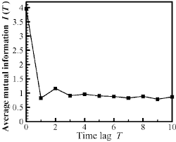
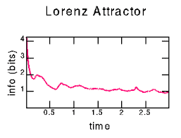
we need to address is the value of the integer “embedding dimension” D. Here is where Whitney’s and Takens’ results come into play. The key idea is that as we enlarge the dimension $D$ of the vector $\mathbf{y}(n)$ we eliminate step by step the intersections of orbits on the system attractor arising from our projection during the measurement process. If this is the case, then there might well be a global dimension allowing us to unfold a particular data set with particular coordinates as entries in $\mathbf{y}(n)$ at a dimension less than the sufficient dimension of the Whitney/Takens geometric result.

To examine this we need the notion of crossing of trajectories, and this we realize in the close analogy of neighbors in the state space which are a result of the dynamics-true neighbors-and neighbors in the state space which are a result of the projection during measurement-false neighbors [23]. If we select an embedding dimension $\mathrm{D}$, then it is a matter of an $\operatorname{order} \mathrm{N} \log (\mathrm{N})$ search among all the points $\mathbf{y}(n)$ in that space to determine the nearest neighbor to a point $\mathbf{y}(\mathrm{k})$. If this nearest neighbor is not a close neighbor in dimension $\mathrm{D}+1$, then its “neighborliness” to $\mathbf{y}(\mathrm{k})$ is the result of a projection from a higher dimensional space. This is a false nearest neighbor, and we wish to eliminate all of them. We accomplish this elimination of the false nearest neighbors by systematically examining the nearest neighbors in dimension $\mathrm{D}$ and their “neighborliness” in dimension D $+1$ for $\mathrm{D}=1,2, \ldots$ until there are no false nearest neighbors remaining. We call this integer dimension $d_E$.

统计代写|时间序列分析代写Time-Series Analysis代考|Local or Dynamical Dimension

The embedding dimension we just selected is a global and average indicator of the number of coordinates needed to unfold the actual data $s(t)$ [24].

The global integer embedding dimension estimate tells us a minimum dimension $d_E$ in which we can place (embed) the signal from our source. This dimension can be larger than the number of degrees of freedom in the dynamics underlying the signal $s(t)$. Suppose that locally the dynamics happened to be a two-dimensional map $\left(x_n, y_n\right) \rightarrow\left(x_{n+1}, y_{n+1}\right)$ but the global structure of the dynamics placed this on the surface of an ordinary torus. To embed the points of the whole data set now lying on a torus, we would have to select $d_E=3$; however, if we wish to determine equations of motion (or a map) to describe the dynamics, we really need only the local dimension of 2 . This local dimension $d_L \leqslant d_E$, and is important when we wish to evaluate the Lyapunov exponent, as we do below, to characterize the dynamical system producing $s(t)$.

To determine $d_L$ we need to move beyond the geometry in the embedding theorem and ask a local question about the data in dimension $\mathrm{d}{\mathrm{E}}$ where we know there are no unwanted intersections of the orbit associated with $s(t)$ and itself. The notion is that data vectors of dimension $\mathrm{d} \leqslant \mathrm{d}{\mathrm{E}}$,
$$
y_d(n)=[s(n), s(n-T), \ldots, s(n-(d-1) T)],
$$
will map without ambiguity locally into other vectors of dimension $d \leqslant d_E$. We can test for this by forming a d-dimensional local map
$$
\mathbf{y}{\mathrm{d}}(\mathrm{n}+1)=\mathbf{M}\left(\mathbf{y}{\mathrm{d}}(\mathrm{n})\right),
$$ and asking whether this map accounts for the behavior of the actual data in $\mathrm{d} \leqslant \mathrm{d}{\mathrm{E}}$. For $\mathrm{d}$ too small, it will not. For $\mathrm{d}=\mathrm{d}{\mathrm{E}}$, it will. If for some intermediate $\mathrm{d}$, the map is accurate, this is an indication of a lower dimensional dynamics than $\mathrm{d}_{\mathrm{E}}$ needed to globally unfold the data.

To answer this question select a data vector $y(k)$ in $d_E$. Select $N_B$ nearest neighbors in phase space to $y(k): y^{(r)}(k) ; r=0,1,2, \ldots, N_B, y^{(0)}(k)=y(k)$. In $\mathrm{d}{\mathrm{E}}$ these are all true neighbors, but their actual time labels may or may not be near the time k. Choose in various ways a d-dimensional subspace of vectors $\mathbf{y}{\mathrm{d}}^{(r)}(\mathrm{k})$. There are $\left(\begin{array}{c}\mathrm{d}_{\mathrm{E}} \ \mathrm{d}\end{array}\right)$ ways to do this and all are worth examining.

时间序列分析代考

统计代写|时间序列分析代写Time-Series Analysis代考|Global Embedding Dimension

下一个关于数据向量的问题
$$
\mathbf{y}(n)=[s(n), s(n-T), \ldots, s(n-(D-1) T)]
$$
我们需要解决的是整数 “嵌入维度” D 的值。这就是 Whitney 和 Takens 的结果发挥作用的地方。关键思想是当我们扩大维度时 $D$ 向量的 $\mathbf{y}(n)$ 我们逐步消除了在测量过程中由我们的投影引起的系统吸引子上的轨道交叉点。如果是这种情况，那么很可能存在一个全局维度，允许我们展开具有特定坐标的特定数据集作为y $\mathbf{y}(n)$ 尺寸小于 Whitney/Takens 几何结果的足够尺寸。
为了检验这一点，我们需要轨迹交叉的概念，并且我们在状态空间中的邻居的密切类比中实现了这一点，这是动态的结果 – 真正的邻居- 和状态空间中的邻居是投影的结果在测量错误的邻居期间 [23]。如果我们选择一个嵌入维度D，那么这是一个问题order $\mathrm{N} \log (\mathrm{N})$ 在所有点中搜索 $\mathbf{y}(n)$ 在该空间中确定点的最近邻居 $\mathbf{y}(\mathrm{k})$. 如果这个最近邻在维度上不是近邻 $\mathrm{D}+1$, 那么它的“邻域”为 $\mathbf{y}(\mathrm{k})$ 是从更高维空间投影的结果。这是一个虚假的最近邻居，我们希望消除所有这些。我们通过系统地检查维度中的最近邻居来完成消除错娱的最近邻居D以及他们在维度 $D$ 中的“邻里关系” $+1$ 为了D $=1,2, \ldots$ 直到没有假的最近邻为止。我们称这个整数维度 $d_E$.

统计代写|时间序列分析代写Time-Series Analysis代考|Local or Dynamical Dimension

我们刚刚选择的嵌入维度是展开实际数据所需的坐标数的全局平均指标 $s(t)$ [24].
全局整数嵌入维数估计告诉我们最小维数 $d_E$ 我们可以在其中放置（嵌入）来自我们来源的信号。该维度可以大于信号基础动力学中的自由度数 $s(t)$. 假设局部动力学恰好是一个二维图 $\left(x_n, y_n\right) \rightarrow\left(x_{n+1}, y_{n+1}\right)$ 但是动力学的全局结构将其置于普通环面的表面上。要嵌入现在位于圆环上的整个数据集的点，我们必须选择 $d_E=3$; 然而，如果我们希望确定运动方程（或映射) 来描述动力学，我们实际上只需要 2 的局部维度。这个局部维度 $d_L \leqslant d_E$ ，并且当我们希望评估 Lyapunov 指数时很重要, 正如我们在下面所做的那样，以表征产生的动力系统s $(t)$.
确定 $d_L$ 我们需要超越嵌入定理中的几何，并提出有关维度数据的局部问题 $\mathrm{dE}$ 我们知道与相关的轨道没有不需要的交叉点 $s(t)$ 和它自己。这个概念是维度的数据向量 $\mathrm{d} \leqslant \mathrm{dE}$ ，
$$
y_d(n)=[s(n), s(n-T), \ldots, s(n-(d-1) T)],
$$
将在本地毫无歧义地映射到其他维度向量 $d \leqslant d_E$. 我们可以通过形成 $d$ 维局部映射来对此进行测试
$$
\mathbf{y d}(\mathrm{n}+1)=\mathbf{M}(\mathbf{y d}(\mathrm{n})),
$$
并询问这张地图是否说明了实际数据的行为 $\mathrm{d} \leqslant \mathrm{dE}$. 为了 $\mathrm{d}$ 太，它不会。为了 $\mathrm{d}=\mathrm{dE}$ ，它会。如果对于一些中间 $d$ ，地图是准确的，这表明比 $\mathrm{d}_{\mathrm{E}}$ 需要在全球展开数据。
要回答这个问题，请选择一个数据向量 $y(k)$ 在 $d_E$. 选择 $N_B$ 相空间中的最近邻 $y(k): y^{(r)}(k) ; r=0,1,2, \ldots, N_B, y^{(0)}(k)=y(k)$. 在 $\mathrm{dE}$ 这些都是真正的邻居，但它们有 $\left(d_E d\right)$ 做到这一点的方法和所有方法都值得研究。

统计代写|时间序列分析代写Time-Series Analysis代考请认准statistics-lab™

统计代写请认准statistics-lab™. statistics-lab™为您的留学生涯保驾护航。

金融工程代写

金融工程是使用数学技术来解决金融问题。金融工程使用计算机科学、统计学、经济学和应用数学领域的工具和知识来解决当前的金融问题，以及设计新的和创新的金融产品。

非参数统计代写

非参数统计指的是一种统计方法，其中不假设数据来自于由少数参数决定的规定模型；这种模型的例子包括正态分布模型和线性回归模型。

广义线性模型代考

广义线性模型（GLM）归属统计学领域，是一种应用灵活的线性回归模型。该模型允许因变量的偏差分布有除了正态分布之外的其它分布。

术语广义线性模型（GLM）通常是指给定连续和/或分类预测因素的连续响应变量的常规线性回归模型。它包括多元线性回归，以及方差分析和方差分析（仅含固定效应）。

有限元方法代写

有限元方法（FEM）是一种流行的方法，用于数值解决工程和数学建模中出现的微分方程。典型的问题领域包括结构分析、传热、流体流动、质量运输和电磁势等传统领域。

有限元是一种通用的数值方法，用于解决两个或三个空间变量的偏微分方程（即一些边界值问题）。为了解决一个问题，有限元将一个大系统细分为更小、更简单的部分，称为有限元。这是通过在空间维度上的特定空间离散化来实现的，它是通过构建对象的网格来实现的：用于求解的数值域，它有有限数量的点。边界值问题的有限元方法表述最终导致一个代数方程组。该方法在域上对未知函数进行逼近。[1] 然后将模拟这些有限元的简单方程组合成一个更大的方程系统，以模拟整个问题。然后，有限元通过变化微积分使相关的误差函数最小化来逼近一个解决方案。

tatistics-lab作为专业的留学生服务机构，多年来已为美国、英国、加拿大、澳洲等留学热门地的学生提供专业的学术服务，包括但不限于Essay代写，Assignment代写，Dissertation代写，Report代写，小组作业代写，Proposal代写，Paper代写，Presentation代写，计算机作业代写，论文修改和润色，网课代做，exam代考等等。写作范围涵盖高中，本科，研究生等海外留学全阶段，辐射金融，经济学，会计学，审计学，管理学等全球99%专业科目。写作团队既有专业英语母语作者，也有海外名校硕博留学生，每位写作老师都拥有过硬的语言能力，专业的学科背景和学术写作经验。我们承诺100%原创，100%专业，100%准时，100%满意。

随机分析代写

随机微积分是数学的一个分支，对随机过程进行操作。它允许为随机过程的积分定义一个关于随机过程的一致的积分理论。这个领域是由日本数学家伊藤清在第二次世界大战期间创建并开始的。

时间序列分析代写

随机过程，是依赖于参数的一组随机变量的全体，参数通常是时间。随机变量是随机现象的数量表现，其时间序列是一组按照时间发生先后顺序进行排列的数据点序列。通常一组时间序列的时间间隔为一恒定值（如1秒，5分钟，12小时，7天，1年），因此时间序列可以作为离散时间数据进行分析处理。研究时间序列数据的意义在于现实中，往往需要研究某个事物其随时间发展变化的规律。这就需要通过研究该事物过去发展的历史记录，以得到其自身发展的规律。

回归分析代写

多元回归分析渐进（Multiple Regression Analysis Asymptotics）属于计量经济学领域，主要是一种数学上的统计分析方法，可以分析复杂情况下各影响因素的数学关系，在自然科学、社会和经济学等多个领域内应用广泛。

MATLAB代写

MATLAB 是一种用于技术计算的高性能语言。它将计算、可视化和编程集成在一个易于使用的环境中，其中问题和解决方案以熟悉的数学符号表示。典型用途包括：数学和计算算法开发建模、仿真和原型制作数据分析、探索和可视化科学和工程图形应用程序开发，包括图形用户界面构建MATLAB 是一个交互式系统，其基本数据元素是一个不需要维度的数组。这使您可以解决许多技术计算问题，尤其是那些具有矩阵和向量公式的问题，而只需用 C 或 Fortran 等标量非交互式语言编写程序所需的时间的一小部分。MATLAB 名称代表矩阵实验室。MATLAB 最初的编写目的是提供对由 LINPACK 和 EISPACK 项目开发的矩阵软件的轻松访问，这两个项目共同代表了矩阵计算软件的最新技术。MATLAB 经过多年的发展，得到了许多用户的投入。在大学环境中，它是数学、工程和科学入门和高级课程的标准教学工具。在工业领域，MATLAB 是高效研究、开发和分析的首选工具。MATLAB 具有一系列称为工具箱的特定于应用程序的解决方案。对于大多数 MATLAB 用户来说非常重要，工具箱允许您学习和应用专业技术。工具箱是 MATLAB 函数（M 文件）的综合集合，可扩展 MATLAB 环境以解决特定类别的问题。可用工具箱的领域包括信号处理、控制系统、神经网络、模糊逻辑、小波、仿真等。

R语言代写	问卷设计与分析代写
PYTHON代写	回归分析与线性模型代写
MATLAB代写	方差分析与试验设计代写
STATA代写	机器学习/统计学习代写
SPSS代写	计量经济学代写
EVIEWS代写	时间序列分析代写
EXCEL代写	深度学习代写
SQL代写	各种数据建模与可视化代写

统计代写|时间序列分析代写Time-Series Analysis代考|STAT758

Posted on 2023年2月9日2023年2月9日 by statistics-lab

如果你也在怎样代写时间序列分析Time-Series Analysis这个学科遇到相关的难题，请随时右上角联系我们的24/7代写客服。

我们提供的时间序列分析Time-Series Analysis及其相关学科的代写，服务范围广, 其中包括但不限于:

Statistical Inference 统计推断
Statistical Computing 统计计算
Advanced Probability Theory 高等概率论
Advanced Mathematical Statistics 高等数理统计学
(Generalized) Linear Models 广义线性模型
Statistical Machine Learning 统计机器学习
Longitudinal Data Analysis 纵向数据分析
Foundations of Data Science 数据科学基础

统计代写|时间序列分析代写Time-Series Analysis代考|STAT758

统计代写|时间序列分析代写Time-Series Analysis代考|Unfolding the Data: Embedding Theorem in Practice

We will primarily focus on the usual and simplest case of time series measurements of a single signal $s(t)$. If more than a single measurement is available, there are additional questions one may ask and answer. The signal is observed with some accuracy, usually specified by an estimate of the “noise” level associated with interference of the measurement by other processes. The signal is also measured in discrete time, starting at an initial time $t_0$ and then typically at a uniform time interval $\tau_s$ we call the sampling time. $s(t)$ is thus the set of $N$ measurements $s\left(t_0+n \tau_s\right), n=1,2, \ldots, N$.

The dynamical system from which the signal comes is usually unknown in detail. In the case of the LP neuron $s(t)$ is the membrane voltage ranging from about $-70 \mathrm{mV}$ to $+50 \mathrm{mV}$, and while one has conductance-based HodgkinHuxley models for the dynamics [8], one does not know how many dynamical variables are needed nor does one know with any specificity the many parameters which enter such models. We are certain, however, that there is more than one dynamical variable and the system state space is not one dimensional even though the measurement is. To describe the state of the system we need more than amplitude and phase which is where linear analyses dwell.

The first task is to ask how many variables we will need to describe the system. If the dynamical system has a state space trajectory lying on an attractor of dimension $d_A$, then our observation is the projection of the multidimensional orbit in a space of integer dimension larger than $\mathrm{d}{\mathrm{A}}$ onto the measurement axis where we observe $s(t)$. If the dynamical system producing $s(t)$ is autonomous, then the orbit does not intersect itself in a high enough dimensional space capturing all the dynamical variables. In a space of integer dimension $\mathrm{D}$ a set of points with dimension $d_A$ intersects itself in a set of points of dimension $d_A+d_A-D$. If $\mathrm{D}$ is large enough, this is negative, indicating no intersections at all. This tells us that if $\mathrm{D}>2 \mathrm{~d}{\mathrm{A}}$, we are guaranteed that the space we use to describe the dynamics will have unfolded the projection made by the measurement. This is a sufficient condition. It could be that a dimension smaller than this unfolds the measurement projection, but we need another tool to determine that $[3,9-16]$.

统计代写|时间序列分析代写Time-Series Analysis代考|Average Mutual Information

The goal of replacing the original signal $s(n)$ with a vector $y(n)$ is to provide independent coordinates in a D-dimensional space to replace the unknown coordinates of the observed system. The components of the vector $\mathbf{y}(n)$ should thus be independent looks at the system itself, so all of the needed dynamical variations in the system are captured. If the time delay between the components $s(n-j T)$ and $s(n-(j-1) T)$ is too small for some $T$, then the components are not really independent and we require a larger $\mathrm{T}$. If $\mathrm{T}$ is too large, then the two measurements $s(n-j T)$ and $s(n-(j-1) T)$ are so far apart in time that the typical instabilities of nonlinear systems will render them essentially uncorrelated. We need some criterion which retains the connection between these measurements yet does not make them essentially identical.

While it is easy to evaluate the linear autocorrelation between measurements as a function of $\mathrm{T}$, the usual criterion of seeking a zero in that quantity only leads to a value of $\mathrm{T}$ where the measurements are linearly independent. The dynamical interest of this is rather small. A much more motivated criterion, though harder to evaluate, was suggested by Fraser and Swinney in 1986: evaluate the average mutual information between measurements at time $n$ and time $n-T$;look for the first minimum in this quantity. This tells us when the two measurements are nenlinearly relatively independent, and this may provide a useful choice for $\mathrm{T}$ [17-21].

时间序列分析代考

统计代写|时间序列分析代写Time-Series Analysis代考|Unfolding the Data: Embedding Theorem in Practice

我们将主要关注单个信号的时间序列测量的常见和最简单的情况 $s(t)$. 如果有多个测量可用，则可能会提出和回答其他问题。观察到的信号具有一定的准确性，通常由与其他过程的测量干扰相关的“噪声”水平的估计来指定。信号也在离散时间测量，从初始时间开始 $t_0$ 然后通常以统一的时间间隔 $\tau_s$ 我们称之为采样时间。 $s(t)$ 因此是一组 $N$ 测量 $s\left(t_0+n \tau_s\right), n=1,2, \ldots, N$.
信号所来自的动力系统的细节通常是末知的。在 LP 神经元的情况下 $s(t)$ 是膜电压范围从约 $-70 \mathrm{mV}$ 到 $+50 \mathrm{mV}$ ，并且虽然有人拥有基于电导的 HodgkinHuxley 动力学模型 [8]，但不知道需要多少动力学变量，也不知道进入此类模型的许多参数的具体情况。然而，我们可以肯定，存在不止一个动力学变量，并且系统状态空间不是一维的，尽管测量是一维的。为了描述系统的状态，我们需要的不仅仅是线性分析所涉及的幅度和相位。
第一项任务是询问我们需要多少变量来描述系统。如果动力系统的状态空间轨迹位于维数吸引子上 $d_A$ ，那么我们的观测就是多维轨道在整数维空间中的投影大于 $\mathrm{dA}$ 在我们观察的测量轴上 $s(t)$. 如果动力系统产生 $s(t)$ 是自主的，那么轨道不会在足够高的维度空间中与自身相交，从而捕获所有的动力学变量。在整数维空间 $\mathrm{D}$ 一组具有维度的点 $d_A$ 在一组维度点中与自身相交 $d_A+d_A-D$. 如果D足够大，这是负数，表示根本没有交叉点。这告诉我们，如果
$\mathrm{D}>2 \mathrm{dA}$ ，我们保证我们用来描述动力学的空间将展开测量所做的投影。这是一个充分条件。可能是比这更小的尺寸展开了测量投影，但我们需要另一种工具来确定 $[3,9-16]$.

统计代写|时间序列分析代写Time-Series Analysis代考|Average Mutual Information

替换原始信号的目标 $s(n)$ 用一个向量 $y(n)$ 就是在D维空间提供独立的坐标来代替被观测系统的末知坐标。向量的组成部分 $\mathbf{y}(n)$ 因此应该独立地观察系统本身，以便捕获系统中所有需要的动态变化。如果组件之间的时间延迟 $s(n-j T)$ 和 $s(n-(j-1) T)$ 对某些人来说太小了 $T$ ，那么组件并不是真正独立的，我们需要一个更大的 $T$. 如果 $T$ 太大，则两次测量
$s(n-j T)$ 和 $s(n-(j-1) T)$ 它们在时间上相距甚远，以至于非线性系统的典型不稳定性将使它们本质上不相关。我们需要一些标准来保留这些测量之间的联系，但又不会使它们本质上相同。
虽然很容易将测量值之间的线性自相关评估为函数 $T$ ，在该数量中寻找零的通常标准只会导致值 T其中测量值是线性独立的。对此的动态兴趣相当小。Fraser 和 Swinney 在 1986 年提出了一个更具动机但更难评估的标准：评估时间测量之间的平均互信息 $n$ 和时间 $n-T$;寻找这个数量的第一个最小值。这告诉我们何时两个测量值呈线性相对独立，这可能会提供一个有用的选择T [17-21].

统计代写请认准statistics-lab™. statistics-lab™为您的留学生涯保驾护航。

金融工程代写

非参数统计代写

非参数统计指的是一种统计方法，其中不假设数据来自于由少数参数决定的规定模型；这种模型的例子包括正态分布模型和线性回归模型。

广义线性模型代考

广义线性模型（GLM）归属统计学领域，是一种应用灵活的线性回归模型。该模型允许因变量的偏差分布有除了正态分布之外的其它分布。

有限元方法代写

随机分析代写

时间序列分析代写

回归分析代写

MATLAB代写

R语言代写	问卷设计与分析代写
PYTHON代写	回归分析与线性模型代写
MATLAB代写	方差分析与试验设计代写
STATA代写	机器学习/统计学习代写
SPSS代写	计量经济学代写
EVIEWS代写	时间序列分析代写
EXCEL代写	深度学习代写
SQL代写	各种数据建模与可视化代写

统计代写|时间序列分析代写Time-Series Analysis代考|STAT3040

Posted on 2022年12月6日2022年12月6日 by statistics-lab

如果你也在怎样代写时间序列分析Time-Series Analysis这个学科遇到相关的难题，请随时右上角联系我们的24/7代写客服。

我们提供的时间序列分析Time-Series Analysis及其相关学科的代写，服务范围广, 其中包括但不限于:

Statistical Inference 统计推断
Statistical Computing 统计计算
Advanced Probability Theory 高等概率论
Advanced Mathematical Statistics 高等数理统计学
(Generalized) Linear Models 广义线性模型
Statistical Machine Learning 统计机器学习
Longitudinal Data Analysis 纵向数据分析
Foundations of Data Science 数据科学基础

统计代写|时间序列分析代写Time-Series Analysis代考|STAT3040

统计代写|时间序列分析代写Time-Series Analysis代考|Decomposition Techniques

Decomposition models in time series are used to identify and describe trend and seasonal factors.
Decomposition means to break down into simpler parts. When decomposition models are used, we can identify these patterns/factors separately.
Some seasonal patterns of a time series model can be describe as festive season effects, holiday effects. As an example think that there is a festive season effect on sales of a textiles company, the company cannot clearly identify how its sales behave in long term. Therefore we can use this method to remove seasonal effects of the time series data set and then try to identify what kind of a trend, these sales have in long term (do the sales increase or decrease annually?)
There are two types of decomposition models. They are additive models and multiplicative models.

Additive model is expressed as: $\mathrm{Y}=\mathrm{T}+\mathrm{S}+\mathrm{C}+\mathrm{I}$.
Multiplicative model is expressed as $\mathrm{Y}=\mathrm{T}^* \mathrm{~S} * \mathrm{C} * \mathrm{I}$. ( $\mathrm{Y}=$ Time Series Data , T=Trend, $\mathrm{S}=$ seasonal , $\mathrm{C}=$ Cynical , $\mathrm{I}=$ Irregular)
Some decomposition models are expressed without cynical patterns. They can be written as below
Additive: $\mathrm{Y}=$ Trend + Seasonal + Irregular
Multiplicative: $\mathrm{Y}=$ Trend $^*$ Seasonal * Irregular
When seasonal variation is relatively constant over time additive model is useful. When seasonal variation is increasing over time multiplicative model is useful. Multiplicative models are useful in economic and business data modeling. The aim of analyzing a time series is to understand and identify the patterns in a time series variable, therefore a variable with more observation outputs better results.
As an example in each year Textiles Pvt Ltd sell cloths worth of $\$ 30000$ in December, where in other months they earn between $\$ 15000$ to $\$ 20000$. Then it is a constant seasonal variation. We can use additive model for this data series.
But if the Textiles Pvt Ltd earns $\$ 30000$ in December 2018, $\$ 40000$ in December $2019, \$ 45000$ in December 2020, and earns between $\$ 15000$ to $\$ 20000$ every other month, then there is a visible increment of seasonal variation. We can use a multiplicative model for this data series.
When multiplicative model $\mathrm{Y}=\mathrm{T}^* \mathrm{~S} * \mathrm{C}^* \mathrm{I}$ is transformed into log, then it becomes $\log \mathrm{Y}=\log \mathrm{T}+\log \mathrm{S}+\log \mathrm{C}+\log \mathrm{I}$.

Graphic method, semi-average method, curve fitting by principles and moving average method are used to measure trend.

统计代写|时间序列分析代写Time-Series Analysis代考|Single Exponential Smoothing

Single exponential smoothing is suitable for the models which don’t show a clear trend or a seasonal pattern. Exponential smoothing is used for forecasting economics and financial data. If there is a time series without a clear pattern then we can use exponential smoothing. But if there is a clear pattern then we should use moving averages.

We can use this method to forecast univariate time series. It can be used as an alternative to ARIMA models. While calculating this model past observations get weighted and they are weighted with a geometrically decreasing ratio. Exponential smooth forecasting is a weighted average forecast of past observations.

In single exponential smoothing, smoothing coefficient is called alpha $\alpha$. Alpha is always between 0 to 1 . Smaller alpha values indicate that there is more impact from past observations. Values close to 1 indicates that only most recent past observations has an influence on the predictions. Alpha is the smoothing constant. Alpha is normally selected between $0.1$ and $0.3$ in practical calculations.

Note: univariate data series is a data series with a single variable. The observations of these data series are recorded according to the time. Example: Annual inflation rate of USA.

Double exponential smoothing is more applicable for univariate data series with trend.
Double exponential smoothing has alpha $\alpha$ and also an additional smoothing factor called $\beta$. Double exponential smoothing with additive trend is referred as Holt’s linear trend model. Double exponential smoothing with an exponential trend is used for the data series with multiplicative trend. These smoothing techniques are used to remove the trend and make the line straight. This method of making the line straight is called damping in time series. This idea was introduced by Gardner \& McKenzie in 1985.

时间序列分析代考

统计代写|时间序列分析代写Time-Series Analysis代考|Decomposition Techniques

时间序列中的分解模型用于识别和描述趋势和季节性因素。
分解意味着分解成更简单的部分。当使用分解模型时，我们可以分别识别这些模式/因素。
时间序列模型的一些季节性模式可以描述为节日效应、假期效应。举个例子，认为节日对一家纺织公司的销售有影响，该公司无法清楚地确定其销售的长期表现。因此，我们可以使用这种方法去除时间序列数据集的季节性影响，然后尝试确定这些销售额在长期内具有什么样的趋势（销售额每年增加还是减少？）
有两种类型的分解模型。它们是加法模型和乘法模型。

加法模型表示为：是=吨+小号+C+我.
乘法模型表示为是=吨∗ 小号∗C∗我. ( 是=时间序列数据，T=趋势，小号=季节性的，C=愤世嫉俗的，我=不规则的）
一些分解模型没有愤世嫉俗的模式。它们可以写成如下
添加剂：是=潮流+季节性+不规则
乘法：是=趋势∗季节性 * 不规则
当季节性变化随时间变化相对恒定时，加法模型很有用。当季节性变化随时间增加时，乘法模型很有用。乘法模型在经济和商业数据建模中很有用。分析时间序列的目的是理解和识别时间序列变量中的模式，因此具有更多观察值的变量输出更好的结果。
例如，每年 Textiles Pvt Ltd 销售的布料价值$30000在 12 月，在其他月份，他们的收入介于$15000至$20000. 然后它是一个恒定的季节性变化。我们可以为这个数据系列使用加法模型。
但如果 Textiles Pvt Ltd 赚$300002018年12月，$40000在十二月2019,$450002020 年 12 月，收入介于$15000至$20000每隔一个月，就会出现明显的季节性变化增量。我们可以为这个数据系列使用乘法模型。
当乘法模型是=吨∗ 小号∗C∗我转化为log，则变为日志⁡是=日志⁡吨+日志⁡小号+日志⁡C+日志⁡我.

采用图形法、半平均法、原理曲线拟合法和移动平均法来衡量趋势。

统计代写|时间序列分析代写Time-Series Analysis代考|Single Exponential Smoothing

单指数平滑适用于没有明显趋势或季节性模式的模型。指数平滑用于预测经济和金融数据。如果时间序列没有明确的模式，那么我们可以使用指数平滑。但如果有一个清晰的模式，那么我们应该使用移动平均线。

我们可以使用这种方法来预测单变量时间序列。它可以用作 ARIMA 模型的替代方案。在计算该模型时，过去的观察值会被加权，并且它们以几何递减的比率加权。指数平滑预测是过去观测值的加权平均预测。

在单指数平滑中，平滑系数称为 alpha一个. Alpha 始终介于 0 到 1 之间。较小的 alpha 值表示过去观察的影响更大。接近 1 的值表示只有最近的过去观察对预测有影响。Alpha 是平滑常数。Alpha 通常选择在0.1和0.3在实际计算中。

注：单变量数据系列是具有单个变量的数据系列。这些数据系列的观察结果是按时间记录的。示例：美国的年通货膨胀率。

双指数平滑更适用于具有趋势的单变量数据序列。
双指数平滑具有 alpha一个还有一个额外的平滑因子称为b. 具有加性趋势的双指数平滑称为 Holt 线性趋势模型。具有指数趋势的双指数平滑用于具有乘法趋势的数据序列。这些平滑技术用于消除趋势并使线条笔直。这种使直线变直的方法在时间序列中称为阻尼。这个想法是由 Gardner \& McKenzie 于 1985 年提出的。

统计代写请认准statistics-lab™. statistics-lab™为您的留学生涯保驾护航。

金融工程代写

非参数统计代写

非参数统计指的是一种统计方法，其中不假设数据来自于由少数参数决定的规定模型；这种模型的例子包括正态分布模型和线性回归模型。

广义线性模型代考

广义线性模型（GLM）归属统计学领域，是一种应用灵活的线性回归模型。该模型允许因变量的偏差分布有除了正态分布之外的其它分布。

有限元方法代写

随机分析代写

时间序列分析代写

回归分析代写

MATLAB代写

R语言代写	问卷设计与分析代写
PYTHON代写	回归分析与线性模型代写
MATLAB代写	方差分析与试验设计代写
STATA代写	机器学习/统计学习代写
SPSS代写	计量经济学代写
EVIEWS代写	时间序列分析代写
EXCEL代写	深度学习代写
SQL代写	各种数据建模与可视化代写

统计代写|时间序列分析代写Time-Series Analysis代考|DSC425

Posted on 2022年12月6日2022年12月6日 by statistics-lab

如果你也在怎样代写时间序列分析Time-Series Analysis这个学科遇到相关的难题，请随时右上角联系我们的24/7代写客服。

我们提供的时间序列分析Time-Series Analysis及其相关学科的代写，服务范围广, 其中包括但不限于:

Statistical Inference 统计推断
Statistical Computing 统计计算
Advanced Probability Theory 高等概率论
Advanced Mathematical Statistics 高等数理统计学
(Generalized) Linear Models 广义线性模型
Statistical Machine Learning 统计机器学习
Longitudinal Data Analysis 纵向数据分析
Foundations of Data Science 数据科学基础

统计代写|时间序列分析代写Time-Series Analysis代考|Moving Average

Moving average method removes short term patterns from a time series. It is a time series smoothing method. Moving average method is better for removing short term patterns.

Moving average is calculated by taking the average for set of observations inside a time series. For a time series with odd numbers of observations Moving average can be calculated by taking the average of 3,5,7 nearby observations. When the numbers of observations are even, then use moving average for time intervals of 2 or 4 . When less observations are taken to count the average, then the line become smoother. That means when a moving average is calculate for time periods of 3 , that line is smoother than a line which is calculated for time periods of 5 . These time intervals are called length of moving average. The length can be 2,3,4,5 or more. But the fitted line is smoother when the length is smaller.

Moving Average method is better than free hand method and semi average method. But when there are outliers or unusual values, this method is not efficient. If there are outliers then it will results unusual curves in the estimated line. Another disadvantage of this method is lacking observations at the first and last places in the newly created array. Now let’s do a sample on simple moving average.

统计代写|时间序列分析代写Time-Series Analysis代考|What is a stationary time series

Stationary Time Series
Stationary time series models are time series that the mean and the variance of the variable don’t depend on the time. Therefore the mean and variance of a stationary time series are constant. They do not have any periodic fluctuations. A stationary time series is simply a stochastic process with constant mean and variance. There are strong stationary series and weak stationary series.
When the distribution of the time series is same as the lagged time series, then it has a strong form of stationary. When the mean and correlation function of a time series does not change by shift in time it is a weak stationary time series. Auto covariance function is not a function of time.
Stationary series is spread around the mean line in a given range. Below is a graph of a stationary time series. Stationary series spread around the mean line in a given range or given upper and lower limits. It has neither trend nor seasonality.

Non Stationary Time Series
Trend, seasonal, cyclic and random patterned series fall under non stationary series. In order to do predictions on a non stationary series, it should be transformed into a stationary series.

Stochastic Process
Stochastic process is a collection of random variables. Time series with the time variable is a basic type of a stochastic process. It is a model for the analysis. This can also be called as random process Mean of a stochastic process $\mu_t=\mathrm{E}\left(y_t\right)$ Where $\mathrm{t}=0, \pm 1, \pm 2 \ldots, \pm \mathrm{n}$
Autocovariance of stochastic process $y_{t, s}=\operatorname{Cov}\left(y_t, y_s\right)$
$\operatorname{Cov}\left(y_t, y_s\right)=\mathrm{E}\left(y_t-\mu_t\right)\left(y_s-\mu_s\right)$
Where $t, s=0, \pm 1, \pm 2 \ldots, \pm n$

时间序列分析代考

统计代写|时间序列分析代写Time-Series Analysis代考|Moving Average

移动平均法从时间序列中移除短期模式。它是一种时间序列平滑方法。移动平均法更适合去除短期形态。

移动平均值是通过对时间序列内的一组观察值取平均值来计算的。对于具有奇数个观测值的时间序列，可以通过取 3、5、7 个附近观测值的平均值来计算移动平均值。当观察次数为偶数时，则对 2 或 4 的时间间隔使用移动平均值。当采用较少的观察来计算平均值时，线条会变得更平滑。这意味着当为 3 的时间段计算移动平均值时，该线比为 5 的时间段计算的线更平滑。这些时间间隔称为移动平均长度。长度可以是2、3、4、5或更多。但当长度较小时，拟合线会更平滑。

移动平均法优于徒手法和半平均法。但当存在异常值或异常值时，这种方法效率不高。如果存在异常值，则会在估计线中产生不寻常的曲线。这种方法的另一个缺点是在新创建的数组的第一个和最后一个位置缺少观察值。现在让我们做一个关于简单移动平均线的示例。

统计代写|时间序列分析代写Time-Series Analysis代考|What is a stationary time series

平稳时间序列
平稳时间序列模型是变量的均值和方差不依赖于时间的时间序列。因此，平稳时间序列的均值和方差是常数。它们没有任何周期性波动。平稳时间序列只是一个具有恒定均值和方差的随机过程。有强平稳序列和弱平稳序列。
当时间序列的分布与滞后时间序列相同时，则具有很强的平稳性。当时间序列的均值和相关函数不随时间变化而变化时，它是一个弱平稳时间序列。自协方差函数不是时间的函数。
平稳序列分布在给定范围内的平均线周围。下面是固定时间序列的图表。平稳序列分布在给定范围或给定上限和下限内的平均线周围。它既没有趋势也没有季节性。

非平稳时间序列
趋势、季节性、周期性和随机模式序列属于非平稳序列。为了对非平稳序列进行预测，应该将其转换为平稳序列。

随机过程
随机过程是随机变量的集合。具有时间变量的时间序列是随机过程的基本类型。它是分析的模型。这也可以称为随机过程随机过程的均值米吨=和(是吨)在哪里吨=0,±1,±2…,±n
随机过程的自协方差是吨,秒=那些⁡(是吨,是秒)
那些⁡(是吨,是秒)=和(是吨−米吨)(是秒−米秒)
在哪里吨,秒=0,±1,±2…,±n

统计代写请认准statistics-lab™. statistics-lab™为您的留学生涯保驾护航。

金融工程代写

非参数统计代写

非参数统计指的是一种统计方法，其中不假设数据来自于由少数参数决定的规定模型；这种模型的例子包括正态分布模型和线性回归模型。

广义线性模型代考

广义线性模型（GLM）归属统计学领域，是一种应用灵活的线性回归模型。该模型允许因变量的偏差分布有除了正态分布之外的其它分布。

有限元方法代写

随机分析代写

时间序列分析代写

回归分析代写

MATLAB代写

R语言代写	问卷设计与分析代写
PYTHON代写	回归分析与线性模型代写
MATLAB代写	方差分析与试验设计代写
STATA代写	机器学习/统计学习代写
SPSS代写	计量经济学代写
EVIEWS代写	时间序列分析代写
EXCEL代写	深度学习代写
SQL代写	各种数据建模与可视化代写

统计代写|时间序列分析代写Time-Series Analysis代考|STAT758

Posted on 2022年12月6日2022年12月6日 by statistics-lab

如果你也在怎样代写时间序列分析Time-Series Analysis这个学科遇到相关的难题，请随时右上角联系我们的24/7代写客服。

我们提供的时间序列分析Time-Series Analysis及其相关学科的代写，服务范围广, 其中包括但不限于:

Statistical Inference 统计推断
Statistical Computing 统计计算
Advanced Probability Theory 高等概率论
Advanced Mathematical Statistics 高等数理统计学
(Generalized) Linear Models 广义线性模型
Statistical Machine Learning 统计机器学习
Longitudinal Data Analysis 纵向数据分析
Foundations of Data Science 数据科学基础

统计代写|时间序列分析代写Time-Series Analysis代考|What is a Time Series

Time series is a collection of observations taken at equal time interval. A time series is a collection of observations or data obtained for a specific variable during a specific, defined and sequence time intervals. In a time series model, observations of a variable are recorded against equal time intervals.

In statistics two types of models are used to analyze data series. They are causal models and time series models. (Regression analysis falls under the category of causal models. In regression analysis, variables are identified as independent and dependent variables.)

If the observations of time periods of $t_1, t_2 \ldots t_n$ are identified as $Y_1, Y_2$ $\ldots Y_n$, then $Y_1, Y_2 \ldots Y_n$ is called a time series. $t_1, t_2 \ldots t_n$ are equal time periods. $Y_1, Y_2 \ldots Y_n$ are observations. $Y_1, Y_2 \ldots Y_n$ is also called an array of time series. Array of time series can be represented by $Y_t\left(Y_t\right.$, where $t=1,2 \ldots n)$.
The function of the relationship between time $(\mathrm{t})$ and the observations of the variable $(\mathrm{Y})$ is $\mathrm{Y}=\mathrm{f}(\mathrm{t})$.
When the time series is lengthy, then the time series analysis is more accurate. But there is short term, medium and long term forecasting methods in time series data analysis. Applying the suitable time series method for the data set increases the accuracy of the analysis.
Uses of Time Series Models
Time series models are useful in studying the past behavior of the variables. It can be used to predict /estimate/forecast the behavior of variables related to business or economy. The time series models can be used to formulate policy decision and future planning. They also can be used to identify interdependencies of two or more time series. Time series data analysis is important to identify underlying forces and structures in a time series variable and to identify a suitable model for forecasting purpose. Future value of a time series can be predicted using present and past observations. The adjacent observations of a time series are dependent. As an example, think about inflation rate of a country, last year’s inflation rate has an influence on this year’s inflation rate and this year’s on next year.

统计代写|时间序列分析代写Time-Series Analysis代考|Time Series Components

It is assumed that fluctuations of a time series are due to coinciding four types of variations. They are

Long Term Trend
Seasonal variation
Cyclical variation
Irregular variations
Above four are called components of a time series. Components of time series are used to describe the variation of a time series. Some argues irregular variations are not a component.
Trend shows a long term increment or decrement of data series.
Seasonal variation show similar repetitive patterns during similar (equivalent) and sequential time periods. In seasonal patterns data series is influenced by seasonally fluctuated data. Seasonal temperature of a country during few years shows seasonal patterns. Cyclic patterns are the alternative upward and downward movements in a time series plot. This can also be identified as recurring sequences of points above and below the trend line lasting at least over one year.

Irregular pattern is a time series with random effect. These types of patterns can happen due to unexpected shocks/influenced/reasons. They can also be identified as residuals or deviations from actual time series. Outliers also fall into this category.

As an example, Sri Lanka had a long term increasing number of foreign tourists, but in 2019 ISIS attacked few tourists’ destinations in Sri Lanka, which caused sudden fall of foreign tourists who are visiting Sri Lanka. This can be identified as an external shock which make the data series irregular.

There are two approaches to describe the relationship among the above components. They are additive models and multiplicative models. These models will be discussed under decomposition methods in this book.

时间序列分析代考

统计代写|时间序列分析代写Time-Series Analysis代考|What is a Time Series

时间序列是在相同时间间隔内进行的观察的集合。时间序列是在特定的、定义的和序列的时间间隔内针对特定变量获得的观察值或数据的集合。在时间序列模型中，变量的观察值是根据相等的时间间隔记录的。

在统计学中，两种类型的模型用于分析数据序列。它们是因果模型和时间序列模型。（回归分析属于因果模型的范畴。在回归分析中，变量被识别为自变量和因变量。）

如果观察时间段吨1,吨2…吨n被确定为是1,是2 …是n，然后是1,是2…是n称为时间序列。吨1,吨2…吨n是相等的时间段。是1,是2…是n是观察。是1,是2…是n也称为时间序列数组。时间序列数组可以表示为是吨(是吨，在哪里吨=1,2…n).
时间关系函数(吨)和变量的观察(是)是是=F(吨).
当时间序列很长时，时间序列分析更准确。但是时间序列数据分析有短期、中期和长期的预测方法。对数据集应用合适的时间序列方法可以提高分析的准确性。
时间序列模型的使用
时间序列模型可用于研究变量的过去行为。它可用于预测/估计/预测与商业或经济相关的变量的行为。时间序列模型可用于制定政策决策和未来规划。它们还可用于识别两个或多个时间序列的相互依赖性。时间序列数据分析对于识别时间序列变量中的潜在力量和结构以及识别用于预测目的的合适模型非常重要。可以使用现在和过去的观察来预测时间序列的未来值。时间序列的相邻观察值是相关的。举个例子，想想一个国家的通货膨胀率，去年的通货膨胀率会影响今年的通货膨胀率，今年的通货膨胀率会影响明年的通货膨胀率。

统计代写|时间序列分析代写Time-Series Analysis代考|Time Series Components

假设时间序列的波动是由于四种类型的变化同时发生。他们是

长期趋势
季节性变化
周期性变化
不规则变化
以上四种称为时间序列的组成部分。时间序列的成分用于描述时间序列的变化。一些人认为不规则的变化不是一个组成部分。
趋势显示数据系列的长期增量或减量。
在相似（等效）和连续的时间段内，季节性变化显示出相似的重复模式。在季节性模式中，数据系列受季节性波动数据的影响。一个国家在几年内的季节性温度显示出季节性模式。循环模式是时间序列图中交替的向上和向下运动。这也可以被识别为至少持续一年以上的趋势线上方和下方点的重复序列。

不规则模式是具有随机效应的时间序列。这些类型的模式可能由于意外的冲击/影响/原因而发生。它们也可以被识别为与实际时间序列的残差或偏差。离群值也属于这一类。

例如，斯里兰卡的外国游客数量长期呈上升趋势，但2019年ISIS袭击斯里兰卡的游客目的地寥寥无几，导致来斯里兰卡的外国游客骤降。这可以被识别为使数据序列不规则的外部冲击。

有两种方法来描述上述组件之间的关系。它们是加法模型和乘法模型。这些模型将在本书的分解方法下进行讨论。

统计代写请认准statistics-lab™. statistics-lab™为您的留学生涯保驾护航。

金融工程代写

非参数统计代写

非参数统计指的是一种统计方法，其中不假设数据来自于由少数参数决定的规定模型；这种模型的例子包括正态分布模型和线性回归模型。

广义线性模型代考

广义线性模型（GLM）归属统计学领域，是一种应用灵活的线性回归模型。该模型允许因变量的偏差分布有除了正态分布之外的其它分布。

有限元方法代写

随机分析代写

时间序列分析代写

回归分析代写

MATLAB代写

R语言代写	问卷设计与分析代写
PYTHON代写	回归分析与线性模型代写
MATLAB代写	方差分析与试验设计代写
STATA代写	机器学习/统计学习代写
SPSS代写	计量经济学代写
EVIEWS代写	时间序列分析代写
EXCEL代写	深度学习代写
SQL代写	各种数据建模与可视化代写

统计代写|时间序列分析代写Time-Series Analysis代考|STAT3040

Posted on 2022年10月18日2022年10月18日 by statistics-lab

如果你也在怎样代写时间序列分析Time-Series Analysis这个学科遇到相关的难题，请随时右上角联系我们的24/7代写客服。

我们提供的时间序列分析Time-Series Analysis及其相关学科的代写，服务范围广, 其中包括但不限于:

Statistical Inference 统计推断
Statistical Computing 统计计算
Advanced Probability Theory 高等概率论
Advanced Mathematical Statistics 高等数理统计学
(Generalized) Linear Models 广义线性模型
Statistical Machine Learning 统计机器学习
Longitudinal Data Analysis 纵向数据分析
Foundations of Data Science 数据科学基础

统计代写|时间序列分析代写Time-Series Analysis代考|STATIONARITY INDUCING TRANSFORMATIONS

2.9 A simple stationarity transformation is to take successive differences of a series, on defining the first-difference of $x_t$ as $\nabla x_t=x_t-x_{t-1}$. Fig. $2.6$ shows the first-differences of the wine and spirits consumption series plotted in Fig. 1.6, that is, the annual changes in consumption. The trends in both series have been eradicated by this transformation and, as will be shown in Chapter 4, ARIMA Models for Nonstationary Time Series, differencing has a lot to recommend it both practically and theoretically for transforming a nonstationary series to stationarity.

First-differencing may, on some occasions, be insufficient to induce stationarity and further differencing may be required. Fig. $2.7$ shows successive temperature readings on a chemical process, this being Series $\mathrm{C}$ of Box and Jenkins (1970). The top panel shows observed temperatures. These display a distinctive form of nonstationarity, in which there are almost random switches in trend and changes in level. Although first differencing (shown as the middle panel) mitigates these switches and changes, it by no means eliminates them; second-differences are required to achieve this, as shown in the bottom panel.
2.10 Some caution is required when taking higher-order differences. The second-differences shown in Fig. $2.7$ are defined as the first-difference of the first-difference, that is, $\nabla \nabla x_t=\nabla^2 x_t$. To provide an explicit expression for second-differences, it is convenient to introduce the lag operator $B$, defined such that $B^i x_t \equiv x_{t-j}$, so that:
$$
\nabla x_t=x_t-x_{t-1}=x_t-B x_t=(1-B) x_t
$$
Consequently:
$$
\nabla^2 x_t=(1-B)^2 x_t=\left(1-2 B+B^2\right) x_t=x_t-2 x_{t-1}+x_{t-2}
$$
which is clearly not the same as $x_t-x_{t-2}=\nabla_2 x_t$, the two-period difference, where the notation $\nabla_j=1-B^j$ for the taking of $j$-period differences has been introduced. The distinction between the two is clearly demonstrated in Fig. 2.8, where second- and two-period differences of Series $\mathrm{C}$ are displayed.
2.11 For some time series, interpretation can be made easier hy taking proportional or percentage changes rather than simple differences, that is, transforming by $\nabla x_t / x_{t-1}$ or $100 \nabla x_t / x_{t-1}$. For financial time series these are typically referred to as the return. Fig. $2.9$ plots the monthly price of gold and its percentage return from 1980 to 2017 .

统计代写|时间序列分析代写Time-Series Analysis代考|DECOMPOSING A TIME SERIES AND SMOOTHING TRANSFORMATIONS

2.17 WMAs may also arise when a simple MA with an even number of terms is used but centering is required. For example, a four-term MA may be defined as:
$$
\mathrm{MA}{t-1 / 2}(4)=\frac{1}{4}\left(x{t-2}+x_{t-1}+x_t+x_{t+1}\right)
$$
where the notation makes clear that the “central” date to which the MA relates to is a noninteger, being halfway between $t-1$ and $t$, that is, $t-(1 / 2)$, but of course $x_{t-(1 / 2)}$ does not exist and the centering property is lost. At $t+1$, however, the MA is:
$$
\operatorname{MA}{t+(1 / 2)}(4)=\frac{1}{4}\left(x{t-1}+x_t+x_{t+1}+x_{t+2}\right)
$$
which has a central date of $t+(1 / 2)$. Taking the average of these two simple MAs produces a weighted MA centered on the average of $t-(1 / 2)$ and $t+(1 / 2)$, which is, of course, $t$ :
$$
\mathrm{WMA}t(5)=\frac{1}{8} x{t-2}+\frac{1}{4} x_{t-1}+\frac{1}{4} x_t+\frac{1}{4} x_{t+1}+\frac{1}{8} x_{t+2}
$$
This is an example of (2.9) with $n=2$ and where there are “half-weights” on the two extreme observations of the MA.
2.18 Fig. $2.12$ plots two simple MAs for the daily observations on the $\$-£$ exchange rate shown in Fig. 1.5. The centered $\operatorname{MA}(251)$ has a span of approximately one year, while the backward looking one-sided MA(60) has a span stretching back over the last three months (5-day working weeks and 20-day working months being assumed here). Naturally, the former MA is much smoother, missing out on the sharper peaks and troughs captured by the latter, but reproducing the longer-term undulations of the exchange rate, known as “long swings.” It also loses the last 125 days (approximately 6 months), which might be regarded as a drawback if recent movements are thought to be of special importance.
2.19 Weighted MAs lie behind many of the trend filters that have been proposed over the years and which will be introduced in Chapter 8, Unobserved Component Models, Signal Extraction, and Filters: see Mills (2011, chapter 10) for a historical discussion. Fig. $2.13$ shows the global temperature series originally plotted in Fig. $1.8$ with a popular trend filter, known as the Hodrick-Prescott (H-P) filter, superimposed. Details of this filter are provided in $\$ \$ 8.13-8.18$, it being a symmetric weighted MA with end-point corrections that allow the filter to be computed right up to the end of the sample, thus avoiding any loss of observations. This is important here, because global temperatures are quite volatile and extracting the recent trend is essential for providing an indication of the current extent of any global warming. The weights of the MA depend on choosing a value for the smoothing parameter: here a large value has been chosen to produce a relatively “smooth trend” that focuses on the longer run movements in temperature.

时间序列分析代考

统计代写|时间序列分析代写Time-Series Analysis代考| stationary arity induced transformation

. txt

一个简单的平稳性变换是取一个级数的连续差分，将$x_t$的一阶差分定义为$\nabla x_t=x_t-x_{t-1}$。图$2.6$显示了图1.6中绘制的葡萄酒和烈酒消费序列的一阶差异，即消费的年度变化。这两个序列中的趋势都被这种转换消除了，正如第4章“非平稳时间序列的ARIMA模型”所示，差分法在将非平稳序列转换为平稳序列的实践和理论上都有很大的可取之处

在某些情况下，一阶差分可能不足以诱导平稳，可能需要进一步差分。图$2.7$显示了化学过程的连续温度读数，这是Box和Jenkins(1970)的$\mathrm{C}$系列。上面的面板显示了观测到的温度。它们表现出一种独特的非平稳形式，其中趋势和水平的变化几乎是随机的开关。尽管第一个差异(如中间面板所示)缓解了这些切换和变化，但它绝不能消除它们;
2.10在取高阶差分时需要谨慎。图$2.7$所示的二次差分定义为第一次差分的第一次差分，即$\nabla \nabla x_t=\nabla^2 x_t$。为了提供二次差的显式表达式，可以方便地引入滞后算符$B$，它被定义为$B^i x_t \equiv x_{t-j}$，从而:
$$
\nabla x_t=x_t-x_{t-1}=x_t-B x_t=(1-B) x_t
$$
因此:
$$
\nabla^2 x_t=(1-B)^2 x_t=\left(1-2 B+B^2\right) x_t=x_t-2 x_{t-1}+x_{t-2}
$$
，这显然与两个周期差的$x_t-x_{t-2}=\nabla_2 x_t$不同，这里引入了用于取$j$ -周期差的符号$\nabla_j=1-B^j$。这两者之间的区别如图2.8所示，其中显示了系列$\mathrm{C}$的第二个和两个周期的差异。对于某些时间序列，通过采用比例或百分比的变化而不是简单的差异，即通过$\nabla x_t / x_{t-1}$或$100 \nabla x_t / x_{t-1}$进行转换，可以使解释更容易。对于金融时间序列，这通常被称为收益。图$2.9$绘制了1980 – 2017年黄金月度价格及其百分比回报率

统计代写|时间序列分析代写时间序列分析代考|分解时间序列和平滑转换

当使用偶数个术语的简单MA但需要定心时，也可能出现wma。例如，一个四项的MA可以定义为:
$$
\mathrm{MA}{t-1 / 2}(4)=\frac{1}{4}\left(x{t-2}+x_{t-1}+x_t+x_{t+1}\right)
$$
，其中符号清楚地表明，MA所涉及的“中心”日期是一个非整数，位于$t-1$和$t$的中间，即$t-(1 / 2)$，但是当然$x_{t-(1 / 2)}$不存在，中心属性丢失。但是在$t+1$, MA是:
$$
\operatorname{MA}{t+(1 / 2)}(4)=\frac{1}{4}\left(x{t-1}+x_t+x_{t+1}+x_{t+2}\right)
$$
，它的中心日期是$t+(1 / 2)$。取这两个简单的MAs的平均值会产生一个以$t-(1 / 2)$和$t+(1 / 2)$的平均值为中心的加权MA，当然，这是$t$:
$$
\mathrm{WMA}t(5)=\frac{1}{8} x{t-2}+\frac{1}{4} x_{t-1}+\frac{1}{4} x_t+\frac{1}{4} x_{t+1}+\frac{1}{8} x_{t+2}
$$
这是(2.9)的一个例子，$n=2$，在MA的两个极端观测值上有“半权值”。
2.18图$2.12$绘制了图1.5中所示$\$-£$汇率每日观测值的两个简单MA。中间的$\operatorname{MA}(251)$的跨度大约为一年，而向后看的单侧MA(60)的跨度可以追溯到过去的三个月(这里假设为5天工作周和20天工作月)。自然，前一个MA要平滑得多，没有后者捕捉到的尖峰和波谷，而是再现了汇率的长期波动，即“长期波动”。它也失去了过去的125天(大约6个月)，如果最近的移动被认为是特别重要的，这可能被视为一个缺点。加权MAs隐藏在许多趋势过滤器的背后，这些趋势过滤器多年来一直被提出，将在第8章，未观测组件模型，信号提取和过滤器中介绍:参见Mills(2011，第10章)进行历史讨论。图$2.13$显示了最初绘制在图$1.8$中的全球温度序列，其中叠加了一个流行的趋势滤波器，即Hodrick-Prescott (hp)滤波器。该滤波器的详细信息在$\$ \$ 8.13-8.18$中提供，它是一个带有端点修正的对称加权MA，允许在样本结束前计算滤波器，从而避免任何观测损失。这一点在这里很重要，因为全球温度是非常不稳定的，提取最近的趋势对于提供任何全球变暖当前程度的指示是至关重要的。MA的权重取决于为平滑参数选择一个值:这里选择了一个较大的值，以产生一个相对“平滑的趋势”，关注温度的长期运动

统计代写请认准statistics-lab™. statistics-lab™为您的留学生涯保驾护航。

金融工程代写

非参数统计代写

非参数统计指的是一种统计方法，其中不假设数据来自于由少数参数决定的规定模型；这种模型的例子包括正态分布模型和线性回归模型。

广义线性模型代考

广义线性模型（GLM）归属统计学领域，是一种应用灵活的线性回归模型。该模型允许因变量的偏差分布有除了正态分布之外的其它分布。

有限元方法代写

随机分析代写

时间序列分析代写

回归分析代写

MATLAB代写

R语言代写	问卷设计与分析代写
PYTHON代写	回归分析与线性模型代写
MATLAB代写	方差分析与试验设计代写
STATA代写	机器学习/统计学习代写
SPSS代写	计量经济学代写
EVIEWS代写	时间序列分析代写
EXCEL代写	深度学习代写
SQL代写	各种数据建模与可视化代写

统计代写|时间序列分析代写Time-Series Analysis代考|DSC425

Posted on 2022年10月18日2022年10月18日 by statistics-lab

如果你也在怎样代写时间序列分析Time-Series Analysis这个学科遇到相关的难题，请随时右上角联系我们的24/7代写客服。

我们提供的时间序列分析Time-Series Analysis及其相关学科的代写，服务范围广, 其中包括但不限于:

Statistical Inference 统计推断
Statistical Computing 统计计算
Advanced Probability Theory 高等概率论
Advanced Mathematical Statistics 高等数理统计学
(Generalized) Linear Models 广义线性模型
Statistical Machine Learning 统计机器学习
Longitudinal Data Analysis 纵向数据分析
Foundations of Data Science 数据科学基础

统计代写|时间序列分析代写Time-Series Analysis代考|TIME SERIES HAVING NATURAL CONSTRAINTS

1.16 Some time series have natural constraints placed upon them. Fig. 1.11, for example, shows the consumption (c), investment $(i)$, government $(g)$, and “other” $(x)$ shares in the United Kingdom’s gross final expenditure for the period $1955 \mathrm{q} 1$ to $2017 \mathrm{q} 2$. Because these shares must be lie between zero and one and must also add up to one for each observation, these restrictions need to be accounted for, as to ignore them would make standard analysis of covariances and correlations invalid. Such compositional time series require distinctive treatment through special transformations before they can be analyzed, as is done in Chapter 16, Compositional and Count Time Series.
1.17 All the time series introduced so far may be regarded as being measured on a continuous scale, or at least can be assumed to be wellapproximated as being continuous. Some series, however, occur naturally as (small) integers and these are often referred to as counts. Fig. $1.12$ shows the annual number of North Atlantic storms and hurricanes (the latter being a subset of the former) between 1851 and 2017. The annual number of storms ranges from a minimum of one (in 1914) to a maximum of 28 in 2005; that year also saw the maximum number of hurricanes, 15, while there were no hurricanes in either 1907 and 1914. The figure uses spike graphs to emphasize the integer nature of these time series and this feature requires special techniques to analyze count data successfully, and will be discussed in Chapter 16, Compositional and Count Time Series.
1.18 Understanding the features exhibited by time series, both individually and in groups, is a key step in their successful analysis and clearly a great deal can be learnt by an initial plot of the data. Such plots may also suggest possible transformations of the data which may expedite formal analysis and modeling of time series, and it is to this topic that Chapter 2, Transforming Time Series, is devoted.

统计代写|时间序列分析代写Time-Series Analysis代考|DISTRIBUTIONAL TRANSFORMATIONS

2.2 Many statistical procedures perform more effectively on data that are normally distributed, or at least are symmetric and not excessively kurtotic (fat-tailed), and where the mean and variance are approximately constant. Observed time series frequently require some form of transformation before they exhibit these distributional properties, for in their “raw” form they are often asymmetric. For example, if a series is only able to take positive (or at least nonnegative) values, then its distribution will usually be skewed to the right, because although there is a natural lower bound to the data, often zero, no upper bound exists and the values are able to “stretch out,” possibly to infinity. In this case a simple and popular transformation is to take logarithms, usually to the base $e$ (natural logarithms).
2.3 Fig. $2.1$ displays histograms of the levels and logarithms of the monthly UK retail price index (RPI) series plotted in Fig. 1.7. Taking logarithms clearly reduces the extreme right-skewness found in the levels, but it certainly does not induce normality, for the distribution of the logarithms is distinctively bimodal.

The reason for this is clearly seen in Fig. 2.2, which shows a time series plot of the logarithms of the RPI. The central part of the distribution, which has the lower relative frequency, is transited swiftly during the 1970s, as this was a decade of high inflation characterized by the steepness of the slope of the series during this period.

Clearly, transforming to logarithms does not induce stationarity, but on comparing Fig. $2.2$ with Fig. 1.7, taking logarithms does “straighten out” the trend, at least to the extent that the periods before 1970 and after 1980 are both approximately linear with roughly the same slope. ${ }^1$ Taking logarithms also stabilizes the variance. Fig. $2.3$ plots the ratio of cumulative standard deviations, $s_i(\mathrm{RPI}) / s_i(\log \mathrm{RPI})$, defined using (1.2) and (1.3) as:
$$
s_i^2(x)=i^{-1} \sum_{t=1}^i\left(x_t-\bar{x}i\right)^2 \quad \bar{x}_i=i^{-1} \sum{t=1}^i x_t
$$ Since this ratio increases monotonically throughout the observation period, the logarithmic transformation clearly helps to stabilize the variance and it will, in fact, do so whenever the standard deviation of a series is proportional to its level. ${ }^2$

时间序列分析代考

统计代写|时间序列分析代写时间序列分析代考|具有自然约束的时间序列

有些时间序列具有自然的约束条件。例如，图1.11显示了$1955 \mathrm{q} 1$至$2017 \mathrm{q} 2$期间英国最终支出总额中的消费(c)、投资$(i)$、政府$(g)$和“其他”$(x)$份额。因为这些份额必须在0和1之间，并且每次观察的总和必须为1，所以需要考虑这些限制，因为忽略它们将使标准的协方差和相关性分析无效。这样的合成时间序列需要通过特殊的变换进行特殊的处理，然后才能进行分析，如第16章“合成和计数时间序列”中所做的。到目前为止介绍的所有时间序列都可以被视为在连续的尺度上测量的，或者至少可以假设很接近连续的。然而，有些级数自然地以(小)整数的形式出现，这些通常称为计数。图$1.12$显示了1851年至2017年间北大西洋风暴和飓风(后者是前者的一个子集)的年度数量。每年的风暴次数从最少的一次(1914年)到最多的28次(2005年)不等;那一年也是飓风数量最多的一年，有15次，而1907年和1914年都没有飓风。该图使用峰值图来强调这些时间序列的整数性质，而这种特征需要特殊的技术来成功地分析计数数据，这将在第16章“组成和计数时间序列”中讨论。理解时间序列所显示的特征，无论是单独的还是分组的，是成功分析的关键步骤，很明显，通过数据的初始绘图可以了解大量信息。这样的图还可能表明数据的可能转换，这可能加快时间序列的形式化分析和建模，第二章“转换时间序列”专门讨论这个主题

统计代写|时间序列分析代写Time-Series Analysis代考|DISTRIBUTIONAL transforms

对于正态分布的数据，或者至少是对称的且不是过度峰度(胖尾)的数据，以及均值和方差近似恒定的数据，许多统计过程可以更有效地执行。观察到的时间序列通常需要某种形式的变换才能表现出这些分布特性，因为在它们的“原始”形式中，它们通常是不对称的。例如，如果一个序列只能取正(或至少是非负的)值，那么它的分布通常会向右倾斜，因为尽管数据有一个自然的下界，通常是零，但不存在上界，值可以“延伸”，可能是无穷大。在这种情况下，一个简单而流行的变换是取对数，通常取底数 $e$ (自然对数)
$2.1$ 显示了英国零售价格指数(RPI)系列的水平和对数的直方图，如图1.7所示。取对数显然减少了在水平中发现的极端右偏性，但它肯定不能诱导正态性，因为对数的分布明显是双峰的

这种情况的原因在图2.2中可以清楚地看到，图2.2显示了RPI对数的时间序列图。分布的中心部分相对频率较低，在1970年代期间迅速过渡，因为这是一个高通货膨胀的十年，其特征是在这一时期系列的斜率非常陡峭

显然，转换为对数并不会导致平稳，但将图$2.2$与图1.7进行比较，取对数确实“理顺”了趋势，至少在1970年之前和1980年之后的时期都近似线性，斜率大致相同的程度上是这样。${ }^1$取对数也能稳定方差。图$2.3$绘制了累积标准差的比值$s_i(\mathrm{RPI}) / s_i(\log \mathrm{RPI})$，使用(1.2)和(1.3)定义为:
$$
s_i^2(x)=i^{-1} \sum_{t=1}^i\left(x_t-\bar{x}i\right)^2 \quad \bar{x}_i=i^{-1} \sum{t=1}^i x_t
$$由于这个比值在整个观察期间是单调增加的，对数变换显然有助于稳定方差，事实上，每当一个系列的标准差与它的水平成正比时，它就会这样做。${ }^2$

统计代写请认准statistics-lab™. statistics-lab™为您的留学生涯保驾护航。

金融工程代写

非参数统计代写

非参数统计指的是一种统计方法，其中不假设数据来自于由少数参数决定的规定模型；这种模型的例子包括正态分布模型和线性回归模型。

广义线性模型代考

广义线性模型（GLM）归属统计学领域，是一种应用灵活的线性回归模型。该模型允许因变量的偏差分布有除了正态分布之外的其它分布。

有限元方法代写

随机分析代写

时间序列分析代写

回归分析代写

MATLAB代写

R语言代写	问卷设计与分析代写
PYTHON代写	回归分析与线性模型代写
MATLAB代写	方差分析与试验设计代写
STATA代写	机器学习/统计学习代写
SPSS代写	计量经济学代写
EVIEWS代写	时间序列分析代写
EXCEL代写	深度学习代写
SQL代写	各种数据建模与可视化代写

统计代写|时间序列分析代写Time-Series Analysis代考|STAT758

Posted on 2022年10月18日2022年10月18日 by statistics-lab

如果你也在怎样代写时间序列分析Time-Series Analysis这个学科遇到相关的难题，请随时右上角联系我们的24/7代写客服。

我们提供的时间序列分析Time-Series Analysis及其相关学科的代写，服务范围广, 其中包括但不限于:

Statistical Inference 统计推断
Statistical Computing 统计计算
Advanced Probability Theory 高等概率论
Advanced Mathematical Statistics 高等数理统计学
(Generalized) Linear Models 广义线性模型
Statistical Machine Learning 统计机器学习
Longitudinal Data Analysis 纵向数据分析
Foundations of Data Science 数据科学基础

统计代写|时间序列分析代写Time-Series Analysis代考|Time Series and Their Features

1.1 As stated in the Introduction, time series are indeed ubiquitous, appearing in almost every research field where data are analyzed. However, their formal study requires special statistical concepts and techniques without which erroneous inferences and conclusions may all too readily be drawn, a problem that statisticians have found necessary to confront since at least Udny Yule’s Presidential Address to the Royal Statistical Society in 1925, provocatively titled “Why do we sometimes get nonsense-correlations between time series? A study in sampling and the nature of time series.” 1
1.2 In general, a time series on some variable $x$ will be denoted as $x_t$, where the subscript $t$ represents time, with $t=1$ being the first observation available on $x$ and $t=T$ being the last. The complete set of times $t=1,2, \ldots, T$ will often be referred to as the observation period. The observations are typically measured at equally spaced intervals, say every minute, hour, or day, etc., so the order in which observations arrive is paramount. This is unlike, say, data on a cross section of a population taken at a given point in time, where the ordering of the data is usually irrelevant unless some form of spatial dependence exists between observations. ${ }^2$
1.3 Time series display a wide variety of features and an appreciation of these is essential for understanding both their properties and their evolution, including calculating future forecasts and, therefore, unknown values of $x_t$ at, say, times $T+1, T+2, \ldots, T+h$, where $h$ is referred to as the forecast horizon.

Fig. $1.1$ shows monthly observations of an index of the North Atlantic Oscillation (NAO) between 1950 and 2017. The NAO is a weather phenomenon in the North Atlantic Ocean and measures fluctuations in the difference of atmospheric pressure at sea level between two stable air pressure areas, the Subpolar low and the Subtropical (Azores) high. Strong positive phases of the NAO tend to be associated with above-normal temperatures in eastern United States and across northern Europe and with below-normal temperatures in Greenland and across southern Europe and the Middle East. These positive phases are also associated with above-normal precipitation over northern Europe and Scandinavia and with below-normal precipitation over southern and central Europe. Upposite patterns of temperature and precipitation anomalies are typically observed during strong negative phases of the NAO (see Hurrell et al., 2003).

Clearly, being able to identify recurring patterns in the NAO would be very useful for medium- to long-range weather forecasting, but, as Fig. $1.1$ illustrates, no readily discernible patterns seem to exist.

统计代写|时间序列分析代写Time-Series Analysis代考|AUTOCORRELATION AND PERIODIC MOVEMENTS

1.4 Such a conclusion may, however, be premature for there might well be internal correlations within the index that could be useful for identifying interesting periodic movements and for forecasting future values of the index. These are typically referred to as the autocorrelations between a current value, $x_t$, and previous, or lagged, values, $x_{t-k}$, for $k=1,2, \ldots$ The lag- $k$ (sample) autocorrelation is defined as
$$
r_k=\frac{\sum_{t=k+1}^T\left(x_t-\bar{x}\right)\left(x_{t-k}-\bar{x}\right)}{T s^2}
$$

where
$$
\bar{x}=T^{-1} \sum_{t=1}^T x_t
$$
and
$$
s^2=T^{-1} \sum_{t=1}^T\left(x_t-\bar{x}\right)^2
$$
are the sample mean and variance of $x_t$, respectively. The set of sample autocorrelations for various values of $k$ is known as the sample autocorrelation function (SACF) and plays a key role in time series analysis. An examination of the SACF of the NAO index is provided in Example 3.1.
1.5 A second physical time series that has a much more pronounced periodic movement is the annual sunspot number from 1700 to 2017 as shown in Fig. 1.2. As has been well-documented, sunspots display a periodic cycle (the elapsed time from one minimum (maximum) to the next) of approximately 11 years; see, for example, Hathaway (2010). The SACF can be used to calculate an estimate of the length of this cycle, as is done in Example 3.3.
1.6 Fig. $1.3$ shows the temperature of a hospital ward taken every hour for several months during 2011 and 2012 (see Iddon et al., 2015, for more details and description of the data). Here there is a long cyclical movement-an annual swing through the seasons-superimposed upon which are short-term diurnal movements as well as a considerable amount of random fluctuation (known as noise), typically the consequence of windows being left open on the ward for short periods of time and more persistent movements which are related to external temperatures and solar irradiation (sunshine).

时间序列分析代考

统计代写|时间序列分析代写时间序列分析代考|时间序列及其特征

1.1如导言所述，时间序列确实是无处不在的，几乎出现在每一个分析数据的研究领域。然而，他们的正式研究需要特殊的统计概念和技术，没有这些概念和技术，就很容易得出错误的推论和结论。至少从1925年乌德尼·尤尔(Udny Yule)在皇家统计学会(Royal statistical Society)发表主席演讲以来，统计学家就发现有必要面对这个问题，该演讲的标题颇具挑衅意味:“为什么我们有时会在时间序列之间得到无意义的相关性?”一项关于采样和时间序列性质的研究。”1
1.2一般来说，一个关于某个变量的时间序列 $x$ 将表示为 $x_t$，其中下标 $t$ 表示时间，其中 $t=1$ 作为第一个观察到的 $x$ 和 $t=T$ 最后一个。全套的时间 $t=1,2, \ldots, T$ 通常被称为观察期。这些观测通常是在等距间隔的时间内进行测量的，比如每分钟、每小时或每一天等，因此观测的到达顺序是最重要的。这与在给定时间点上采集的种群横截面数据不同，后者数据的顺序通常是不相关的，除非观察之间存在某种形式的空间依赖性。 ${ }^2$时间序列显示出各种各样的特征，对这些特征的认识对于理解它们的性质和演变是至关重要的，包括计算未来的预测，以及因此的未知值 $x_t$ 在，比如说，几次 $T+1, T+2, \ldots, T+h$，其中 $h$ 称为预测层位。

$1.1$显示了1950年至2017年期间北大西洋涛动指数(NAO)的月度观测结果。NAO是北大西洋的一种天气现象，测量两个稳定气压区(亚极地低压区和亚热带(亚速尔群岛)高压区)之间的海平面大气压力差的波动。NAO的强正相位往往与美国东部和整个北欧的高于正常温度有关，与格陵兰岛和整个南欧和中东的低于正常温度有关。这些正相也与北欧和斯堪的那维亚半岛上空高于正常的降水和南欧和中欧上空低于正常的降水有关。温度和降水异常的反向模式通常在NAO的强负相期间观察到(见Hurrell等人，2003年) 显然，能够识别NAO中反复出现的模式对中期到长期天气预报非常有用，但是，如图$1.1$所示，似乎不存在容易识别的模式

统计代写|时间序列分析代写Time-Series Analysis代考|AUTOCORRELATION AND PERIODIC movement

1.4然而，这样的结论可能还为时过早，因为指数内部很可能存在内在的相互关系，有助于确定有趣的周期性波动和预测指数的未来值。这些通常被称为当前值$x_t$和之前的或滞后的值$x_{t-k}$(用于$k=1,2, \ldots$)之间的自相关性。滞后- $k$(样本)自相关性定义为
$$
r_k=\frac{\sum_{t=k+1}^T\left(x_t-\bar{x}\right)\left(x_{t-k}-\bar{x}\right)}{T s^2}
$$

其中
$$
\bar{x}=T^{-1} \sum_{t=1}^T x_t
$$
和
$$
s^2=T^{-1} \sum_{t=1}^T\left(x_t-\bar{x}\right)^2
$$
分别是$x_t$的样本均值和方差。$k$的各种值的样本自相关集称为样本自相关函数(SACF)，在时间序列分析中起着关键作用。第二个具有更明显的周期性运动的物理时间序列是每年从1700到2017年的太阳黑子数，如图1.2所示。正如文献记载的那样，太阳黑子的周期(从一个最小值(最大值)到下一个最小值的时间)约为11年;比如，海瑟薇(2010)。SACF可用于计算该周期长度的估计，如例3.3所示。图$1.3$显示了2011年和2012年几个月里每小时采集的医院病房温度(有关数据的更多细节和描述，请参见Iddon等人，2015)。这里有一个长期的周期性运动——一年四季的波动——叠加在此之上的是短期的昼夜运动和大量的随机波动(称为噪声)，这通常是病房的窗户短时间开着的结果，以及与外部温度和太阳照射(阳光)有关的更持久的运动

统计代写请认准statistics-lab™. statistics-lab™为您的留学生涯保驾护航。

金融工程代写

非参数统计代写

非参数统计指的是一种统计方法，其中不假设数据来自于由少数参数决定的规定模型；这种模型的例子包括正态分布模型和线性回归模型。

广义线性模型代考

广义线性模型（GLM）归属统计学领域，是一种应用灵活的线性回归模型。该模型允许因变量的偏差分布有除了正态分布之外的其它分布。

有限元方法代写

随机分析代写

时间序列分析代写

回归分析代写

MATLAB代写

R语言代写	问卷设计与分析代写
PYTHON代写	回归分析与线性模型代写
MATLAB代写	方差分析与试验设计代写
STATA代写	机器学习/统计学习代写
SPSS代写	计量经济学代写
EVIEWS代写	时间序列分析代写
EXCEL代写	深度学习代写
SQL代写	各种数据建模与可视化代写

统计代写|时间序列分析代写Time-Series Analysis代考|STAT435

Posted on 2022年9月24日2022年9月24日 by statistics-lab

如果你也在怎样代写时间序列分析Time-Series Analysis这个学科遇到相关的难题，请随时右上角联系我们的24/7代写客服。

我们提供的时间序列分析Time-Series Analysis及其相关学科的代写，服务范围广, 其中包括但不限于:

Statistical Inference 统计推断
Statistical Computing 统计计算
Advanced Probability Theory 高等概率论
Advanced Mathematical Statistics 高等数理统计学
(Generalized) Linear Models 广义线性模型
Statistical Machine Learning 统计机器学习
Longitudinal Data Analysis 纵向数据分析
Foundations of Data Science 数据科学基础

统计代写|时间序列分析代写Time-Series Analysis代考|STAT435

统计代写|时间序列分析代写Time-Series Analysis代考|Seasonal ARIMA Modeling of Beer Sales

The SACF for the $\nabla \nabla^4$ transformation of beer sales shown in Fig. $9.3$ has $r_1=-0.56, r_2=-0.03, r_3=0.44, r_4=-0.65$, and $r_5=0.30$. Since $r_2 \approx 0$ and $r_1 r_4=0.36$, these first five sample autocorrelations are, within reasonable sampling limits, consistent with the ACF of an $\operatorname{ARIMA}(0,1,1)(0,1,1)4$ airline model. Using (9.7) the standard error of the sample autocorrelations for lags greater than 5 is calculated to be $0.20$. Only $r{16}$ exceeds two-standard errors, suggesting that this airline model could represent a satisfactory representation of the beer sales data. Fitting this model obtains ${ }^4$ :
$$
\nabla_1 \nabla_4 x_t=\left(1-\begin{array}{c}
0.694 \
(0.098)
\end{array}\right)\left(1-\begin{array}{c}
0.604 \
(0.110)
\end{array} B^4\right) a_t \quad \hat{\sigma}=271.9
$$
The more general seasonal ARIMA model is estimated to be:
$$
\nabla \nabla_4 x_t=\left(1-\underset{(0.072)}{0.802} B-\underset{(0.095)}{0.552} B^4+\begin{array}{c}
0.631 \
(0.098)
\end{array} B^5\right) a_t \quad \hat{\sigma}=265.0
$$
The multiplicative model imposes the nonlinear restriction $\theta_1 \theta_4+\theta_5=0$. The log-likelihoods of the two models are $-547.76$ and $-545.64$, leading to a likelihood ratio test statistic of $4.24$, which is distributed as chi-square with one degree of freedom and so is not quite significant at the $2.5 \%$ level, although a Wald test does prove to be significant.

Using $\theta=0.7$ and $\Theta=0.6$ for simplicity, then the $\psi$-weights of the airline model are given, in general, by:
$$
\begin{gathered}
\psi_{4 r+1}=\psi_{4 r+2}=\psi_{4(r+1)-1}=0.3(r+1-0.6 r)=0.3+0.12 r \
\psi_{4(r+1)}=0.3(r+1-0.6 r)+0.4=0.7+0.12 r
\end{gathered}
$$
Thus,
$$
\begin{aligned}
&\psi_1=\psi_2=\psi_3=0.3 \
&\psi_4=0.7 \
&\psi_5=\psi_6=\psi_7=0.42 \
&\psi_8=0.82 \
&\psi_9=\psi_{10}=\psi_{11}=0.54, \text { etc. }
\end{aligned}
$$

统计代写|时间序列分析代写Time-Series Analysis代考|SEASONAL ADJUSTMENT

9.13 In $\S 2.16$ we introduced a decomposition of an observed time series into trend, seasonal, and irregular (or noise) components, focusing attention on estimating the seasonal component and then eliminating it to provide a seasonally adjusted series. Extending the notation introduced in (8.1), this implicit UC decomposition can be written as
$$
x_t=z_t+s_t+u_t
$$
where the additional seasonal component $s_t$ is assumed to be independent of both $z_t$ and $u_t$. On obtaining an estimate of the seasonal component, $\hat{s}_t$, the seasonally adjusted series can then be defined as $x_t^a=x_t-\hat{s}_t$.
9.14 An important question is why we would wish to remove the seasonal component, rather than modeling it as an integral part of the stochastic process generating the data, as in fitting a seasonal ARIMA model, for example. A commonly held view is that the ability to recognize, interpret, or react to important nonseasonal movements in a series, such as turning points and other cyclical events, emerging patterns, or unexpected occurrences for which potential causes might be sought, may well be hindered by the presence of seasonal movements. Consequently, seasonal adjustment is carried out to simplify data so that they may be more easily interpreted by “statistically unsophisticated” users without this simplification being accompanied by too large a loss of information.

This qualifier is important because it requires that the seasonal adjustment procedure does not result in a “significant” loss of information. Although the moving average method introduced in $\$ 2.16$ is both intuitively and computationally simple, it may not be the best available method. Historically, seasonal adjustment methods have been categorized as either empirically- or model-based. The moving average method falls into the former category, as are the methods developed by statistical agencies, such as the sequence of procedures developed by the United States Bureau of the Census, the latest incarnation being known as X-13. Model-based methods employ signal extraction techniques based on ARIMA models fitted either to the observed series or to its components. The most popular of these methods is known as TRAMO/SEATS: see Gómez and Maravall (1996) and Mills (2013b). The distinction between empirical and model-based methods is, however, becoming blurred as X-13 also uses ARIMA models in its computations. ${ }^6$

时间序列分析代考

统计代写|时间序列分析代写时间序列分析代考|啤酒销售的季节性ARIMA建模

图$9.3$所示的啤酒销售$\nabla \nabla^4$转型的SACF有$r_1=-0.56, r_2=-0.03, r_3=0.44, r_4=-0.65$，和$r_5=0.30$。从$r_2 \approx 0$和$r_1 r_4=0.36$开始，在合理的抽样范围内，这前五个样本自相关性与$\operatorname{ARIMA}(0,1,1)(0,1,1)4$航空公司模型的ACF一致。使用(9.7)计算滞后大于5的样本自相关的标准误差为$0.20$。只有$r{16}$超过了两个标准误差，这表明这个航空公司模型可以代表一个令人满意的啤酒销售数据的表示。拟合该模型得到${ }^4$:
$$
\nabla_1 \nabla_4 x_t=\left(1-\begin{array}{c}
0.694 \
(0.098)
\end{array}\right)\left(1-\begin{array}{c}
0.604 \
(0.110)
\end{array} B^4\right) a_t \quad \hat{\sigma}=271.9
$$
更一般的季节性ARIMA模型估计为:
$$
\nabla \nabla_4 x_t=\left(1-\underset{(0.072)}{0.802} B-\underset{(0.095)}{0.552} B^4+\begin{array}{c}
0.631 \
(0.098)
\end{array} B^5\right) a_t \quad \hat{\sigma}=265.0
$$
乘法模型施加了非线性约束$\theta_1 \theta_4+\theta_5=0$。两个模型的对数似然是$-547.76$和$-545.64$，导致了$4.24$的似然比检验统计量，它以一个自由度的卡方分布，因此在$2.5 \%$水平上不太显著，尽管Wald检验确实证明显著。

为了简单起见，使用$\theta=0.7$和$\Theta=0.6$，那么航空公司模型的$\psi$ -权重一般由:
$$
\begin{gathered}
\psi_{4 r+1}=\psi_{4 r+2}=\psi_{4(r+1)-1}=0.3(r+1-0.6 r)=0.3+0.12 r \
\psi_{4(r+1)}=0.3(r+1-0.6 r)+0.4=0.7+0.12 r
\end{gathered}
$$
因此，
$$
\begin{aligned}
&\psi_1=\psi_2=\psi_3=0.3 \
&\psi_4=0.7 \
&\psi_5=\psi_6=\psi_7=0.42 \
&\psi_8=0.82 \
&\psi_9=\psi_{10}=\psi_{11}=0.54, \text { etc. }
\end{aligned}
$$

统计代写|时间序列分析代写时间序列分析代考|季节性调整

9.13 In $\S 2.16$ 我们将观察到的时间序列分解为趋势、季节和不规则(或噪声)成分，重点关注估计季节成分，然后消除它，以提供季节性调整的序列。扩展(8.1)中介绍的符号，这个隐式UC分解可以写成
$$
x_t=z_t+s_t+u_t
$$
其中附加的季节性成分 $s_t$ 是独立于两者的吗 $z_t$ 和 $u_t$。在得到季节成分的估计后， $\hat{s}_t$，则季节性调整序列可定义为 $x_t^a=x_t-\hat{s}_t$一个重要的问题是，为什么我们希望删除季节性成分，而不是将其建模为生成数据的随机过程的一个整体部分，例如，在拟合季节性ARIMA模型时。一种普遍的观点认为，识别、解释或对一系列重要的非季节性运动(如转折点和其他周期性事件、新出现的模式或可能寻找潜在原因的意外事件)作出反应的能力很可能会受到季节性运动的存在的阻碍。因此，进行了季节调整，以简化数据，使“统计上不熟练”的用户可以更容易地解释这些数据，而不会伴随这种简化而造成太大的信息损失这个限定符很重要，因为它要求季节调整过程不会导致信息的“重大”损失。虽然$\$ 2.16$中介绍的移动平均方法直观且计算简单，但它可能不是最好的可用方法。历史上，季节性调整方法被分为基于经验和基于模型的两类。移动平均方法属于前一类，由统计机构制定的方法也属于前一类，例如由美国人口普查局制定的一系列程序，其最新版本被称为X-13。基于模型的方法采用基于拟合观测序列或其组成部分的ARIMA模型的信号提取技术。这些方法中最流行的是TRAMO/SEATS:见Gómez和Maravall(1996)和Mills (2013b)。然而，经验方法和基于模型的方法之间的区别正在变得模糊，因为X-13在其计算中也使用ARIMA模型。${ }^6$

统计代写请认准statistics-lab™. statistics-lab™为您的留学生涯保驾护航。

金融工程代写

非参数统计代写

非参数统计指的是一种统计方法，其中不假设数据来自于由少数参数决定的规定模型；这种模型的例子包括正态分布模型和线性回归模型。

广义线性模型代考

广义线性模型（GLM）归属统计学领域，是一种应用灵活的线性回归模型。该模型允许因变量的偏差分布有除了正态分布之外的其它分布。

有限元方法代写

随机分析代写

时间序列分析代写

回归分析代写

MATLAB代写

R语言代写	问卷设计与分析代写
PYTHON代写	回归分析与线性模型代写
MATLAB代写	方差分析与试验设计代写
STATA代写	机器学习/统计学习代写
SPSS代写	计量经济学代写
EVIEWS代写	时间序列分析代写
EXCEL代写	深度学习代写
SQL代写	各种数据建模与可视化代写

统计代写|时间序列分析代写Time-Series Analysis代考|DSC425

Posted on 2022年9月24日2022年9月24日 by statistics-lab

如果你也在怎样代写时间序列分析Time-Series Analysis这个学科遇到相关的难题，请随时右上角联系我们的24/7代写客服。

我们提供的时间序列分析Time-Series Analysis及其相关学科的代写，服务范围广, 其中包括但不限于:

Statistical Inference 统计推断
Statistical Computing 统计计算
Advanced Probability Theory 高等概率论
Advanced Mathematical Statistics 高等数理统计学
(Generalized) Linear Models 广义线性模型
Statistical Machine Learning 统计机器学习
Longitudinal Data Analysis 纵向数据分析
Foundations of Data Science 数据科学基础

统计代写|时间序列分析代写Time-Series Analysis代考|SIGNAL EXTRACTION

8.8 Given a UC model of the form of (8.1) and models for $z_t$ and $u_t$, it is often useful to provide estimates of these two unobserved components, a procedure that is known as signal extraction. A MMSE estimate of $z_t$, is an estimate $\hat{z}t$ which minimizes $E\left(\zeta_t^2\right)$, where $\zeta_t=z_t-\hat{z}_t$ is the estimation error (cf. \$7.2). From, for example. Pierce (1979). given an infinite sample of observations, denoted $\left{x_t,-\infty \leq t \leq \infty\right}$, such an estimator is: $$ \hat{z}_t=\nu_z(B) x_t=\sum{j=-\infty}^{\infty} \nu_{z j} x_{t-j}
$$
where the filter $\nu_z(B)$ is defined as:
$$
\nu_z(B)=\frac{\sigma_v^2 \gamma(B) \gamma\left(B^{-1}\right)}{\sigma_e^2 \theta(B) \theta\left(B^{-1}\right)}
$$
in which case the noise component can be estimated as:
$$
\hat{u}t=x_t-\hat{z}_t=\left(1-\nu_z(B)\right) x_t=\nu_u(B) x_t $$ For example, for the Muth model of a random walk overlaid with white noise: $$ \nu_z(B)=\frac{\sigma_v^2}{\sigma_e^2}(1-\theta B)^{-1}\left(1-\theta B^{-1}\right)^{-1}=\frac{\sigma_v^2}{\sigma_e^2} \frac{1}{\left(1-\theta^2\right)} \sum{j=-\infty}^{\infty} \theta^{|j|} B^j
$$
so that, using $\sigma_v^2=(1-\theta)^2 \sigma_e^2$, obtained using (8.6), we have:
$$
\hat{z}t=\left.\frac{(1-\theta)^2}{1-\theta^2} \sum{j=-\infty}^{\infty} \theta^{\mid j}\right|{x{t-j}}
$$
Thus, for values of $\theta$ close to unity, $\hat{z}_t$ will be given by an extremely long moving average of future and past values of $x$. If $\theta$ is close to zero, however, $\hat{z}_t$ will be almost equal to the most recently observed value of $x$. From (8.3), large values of $\theta$ are seen to correspond to small values of the signal-tonoise variance ratio $\kappa=\sigma_v^2 / \sigma_u^2$. When the noise component dominates, a long moving average of $x$ values will provide the best estimate of the trend, while if the noise component is only small then the trend is essentially given by the current position of $x$.

统计代写|时间序列分析代写Time-Series Analysis代考|MODELING STOCHASTIC SEASONALITY

9.3 It would, however, be imprudent to rule out the possibility of an evolving seasonal pattern: in other words, the presence of stochastic seasonality. As in the modeling of stochastic trends, ARIMA processes have been found to do an excellent job in modeling stochastic seasonality, albeit in an extended form to that developed in previous chapters.
9.4 An important consideration when attempting to model a seasonal time series with an ARIMA model is to determine what sort of process will best match the SACFs and PACFs that characterize the data. Concentrating on the beer sales series, we have already noted the seasonal pattern in the SACF for $\nabla x_t$ shown in Fig. 9.1. In considering the SACF further, we note that the seasonality manifests itself in large positive autocorrelations at the seasonal lags ( $4 k, k \geq 1$ ) being flanked by negative autocorrelations at the “satellites” $[4(k-1), 4(k+1)]$. The slow decline of these seasonal autocorrelations is indicative of seasonal nonstationarity and, analogous to the analysis of “nonseasonal nonstationarity,” this may be dealt with by seasonal differencing, that is, by using the $\nabla_4=1-B^4$ operator in conjunction with the usual $\nabla$ operator. Fig. $9.3$ shows the SACF of $\nabla \nabla^4$ transformed beer sales and this is now clearly stationary and, thus, potentially amenable to ARIMA identification.
9.5 In general, if we have a seasonal period of $m$ then the seasonal differencing operator may be denoted as $\nabla_m$. The nonseasonal and seasonal differencing operators may then be applied $d$ and $D$ times, respectively, so that a seasonal ARIMA model may take the general form
$$
\nabla^d \nabla_m^D \phi(B) x_t=\theta(B) a_t
$$ Appropriate forms of the $\theta(B)$ and $\phi(B)$ polynomials can then, at least in principle, be obtained by the usual methods of identification and/or model selection. Unfortunately, two difficulties are typically encountered. First, the PACFs of seasonal models are difficult both to derive and to interpret, so that conventional identification is usually based solely on the behavior of the appropriate SACF. Second, since the $\theta(B)$ and $\phi(B)$ polynomials need to account for the seasonal autocorrelation, at least one of them must be of minimum order $m$. This often means that the number of models which need to be considered in model selection procedures can become prohibitively large.

时间序列分析代考

统计代写|时间序列分析代写时间序列分析代考|信号提取

给定(8.1)形式的UC模型和$z_t$和$u_t$的模型，提供这两个未观测成分的估计通常是有用的，这个过程被称为信号提取。对$z_t$的MMSE估计是将$E\left(\zeta_t^2\right)$最小化的估计$\hat{z}t$，其中$\zeta_t=z_t-\hat{z}t$是估计误差(cf $7.2)。例如，从。皮尔斯(1979)。给定一个无限的观察样本，记为$\left{x_t,-\infty \leq t \leq \infty\right}$，这样的估计量是:$$ \hat{z}_t=\nu_z(B) x_t=\sum{j=-\infty}^{\infty} \nu{z j} x_{t-j}
$$
，其中滤波器$\nu_z(B)$定义为:
$$
\nu_z(B)=\frac{\sigma_v^2 \gamma(B) \gamma\left(B^{-1}\right)}{\sigma_e^2 \theta(B) \theta\left(B^{-1}\right)}
$$
，在这种情况下，噪声分量可以估计为:
$$
\hat{u}t=x_t-\hat{z}_t=\left(1-\nu_z(B)\right) x_t=\nu_u(B) x_t $$例如，对于覆盖着白噪声的随机漫步的Muth模型:$$ \nu_z(B)=\frac{\sigma_v^2}{\sigma_e^2}(1-\theta B)^{-1}\left(1-\theta B^{-1}\right)^{-1}=\frac{\sigma_v^2}{\sigma_e^2} \frac{1}{\left(1-\theta^2\right)} \sum{j=-\infty}^{\infty} \theta^{|j|} B^j
$$
，因此，使用(8.6)得到的$\sigma_v^2=(1-\theta)^2 \sigma_e^2$，我们有:
$$
\hat{z}t=\left.\frac{(1-\theta)^2}{1-\theta^2} \sum{j=-\infty}^{\infty} \theta^{\mid j}\right|{x{t-j}}
$$
因此，对于$\theta$的值接近于单位，$\hat{z}_t$将由$x$的未来值和过去值的一个极长的移动平均值给出。但是，如果$\theta$接近于零，$\hat{z}_t$将几乎等于$x$最近观察到的值。从(8.3)可以看出，$\theta$的大值对应于信号-噪声方差比$\kappa=\sigma_v^2 / \sigma_u^2$的小值。当噪声分量占主导地位时，$x$值的长移动平均值将提供趋势的最佳估计，而如果噪声分量很小，则趋势基本上由$x$的当前位置给出。

统计代写|时间序列分析代写时间序列分析代考|建模随机季节性

然而，排除一种不断演变的季节模式的可能性是轻率的:换句话说，随机季节性的存在。在随机趋势的建模中，ARIMA过程被发现在建模随机季节性方面做得很好，尽管是在前几章中开发的扩展形式。9.4当试图用ARIMA模型建模季节时间序列时，一个重要的考虑因素是确定哪种过程将最好地匹配描述数据的sacf和pacf。专注于啤酒销售系列，我们已经注意到$\nabla x_t$的SACF的季节性模式，如图9.1所示。在进一步考虑SACF时，我们注意到，季节性表现为在季节性滞后($4 k, k \geq 1$)上有大量的正自相关，而在“卫星”$[4(k-1), 4(k+1)]$上则有负自相关。这些季节性自相关的缓慢下降表明了季节性的非平稳性，并且，类似于“非季节性非平稳性”的分析，这可以通过季节性差异来处理，也就是说，通过将$\nabla_4=1-B^4$算子与通常的$\nabla$算子结合使用。图$9.3$显示了$\nabla \nabla^4$转换后的啤酒销售的SACF，这现在显然是静止的，因此，可能符合ARIMA识别。
9.5一般来说，如果我们有一个$m$的季节性周期，那么季节差异算子可以表示为$\nabla_m$。然后可以分别应用非季节性和季节性差分算子$d$和$D$次，这样季节性ARIMA模型就可以采用一般形式
$$
\nabla^d \nabla_m^D \phi(B) x_t=\theta(B) a_t
$$然后，至少在原则上，可以通过通常的识别和/或模型选择方法得到$\theta(B)$和$\phi(B)$多项式的适当形式。不幸的是，通常会遇到两个困难。首先，季节模型的pacf难以推导和解释，因此传统的识别通常仅基于适当的SACF的行为。其次，由于$\theta(B)$和$\phi(B)$多项式需要考虑季节自相关，它们中至少有一个必须是最小阶$m$。这通常意味着在模型选择过程中需要考虑的模型数量会变得大得令人望而却步

统计代写请认准statistics-lab™. statistics-lab™为您的留学生涯保驾护航。

R语言代写	问卷设计与分析代写
PYTHON代写	回归分析与线性模型代写
MATLAB代写	方差分析与试验设计代写
STATA代写	机器学习/统计学习代写
SPSS代写	计量经济学代写
EVIEWS代写	时间序列分析代写
EXCEL代写	深度学习代写
SQL代写	各种数据建模与可视化代写