如果你也在 怎样代写生物统计biostatistics这个学科遇到相关的难题，请随时右上角联系我们的24/7代写客服。

生物统计学是将统计技术应用于健康相关领域的科学研究，包括医学、生物学和公共卫生，并开发新的工具来研究这些领域。

statistics-lab™ 为您的留学生涯保驾护航 在代写生物统计biostatistics方面已经树立了自己的口碑, 保证靠谱, 高质且原创的统计Statistics代写服务。我们的专家在代写生物统计biostatistics代写方面经验极为丰富，各种生物统计biostatistics相关的作业也就用不着说。

我们提供的生物统计biostatistics及其相关学科的代写，服务范围广, 其中包括但不限于:

• Statistical Inference 统计推断
• Statistical Computing 统计计算
• Advanced Probability Theory 高等概率论
• Advanced Mathematical Statistics 高等数理统计学
• (Generalized) Linear Models 广义线性模型
• Statistical Machine Learning 统计机器学习
• Longitudinal Data Analysis 纵向数据分析
• Foundations of Data Science 数据科学基础

统计代写|生物统计代写biostatistics代考|OBTAINING REPRESENTATIVE DATA

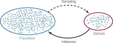
The purpose of sampling is to get a sufficient amount of data that is representative of target population so that statistical inferences can be made about the distribution and the parameters of the target population. Because a sample is only a subset of the units in the target population, it is generally impossible to guarantee that the sample data are representative of the target population; however, with a well-designed sampling plan, it will be unlikely to select a sample that is not representative of the target population. To ensure the likelihood that the sample data will be representative of the target population, the following components of the sampling process must be considered:

• Target Population The target population must be well defined, accessible, and the researcher should have a good understanding of the structure of the population. In particular, the researcher should be able to identify the units of the population, the approximate number of units in the population, subpopulations, the approximate shape of the distributions of the variables being studied, and the relevant parameters that need to be estimated.
• Sampling Units The Sampling units are the units of the population that will be sampled. A sampling unit may or may not be a unit of the population. In fact, in some sampling plans, the sampling unit is a collection of population units. The sampling unit is also the smallest unit in the target population that can be selected.
• Sampling Element A sampling element is an object on which measurements will be made. A sampling element may or may not be a sampling unit. When the sampling unit consists of several population units, it is called a cluster of units. If each

population unit in a cluster will be measured, then the sampling elements are the population units within the sampled clusters. In this case, the sampling element is a subunit of the sampling unit.

• Sampling Frame The sampling frame is the list of sampling units that are available for sampling. The sampling frame should be nearly equal to the target population. When the sampling frame is significantly different from the target population, it makes it less unlikely that a sample representative of the target population will be obtained, even with a well-designed sampling plan. Sampling frames that fail to include all of the units of the target population are said to undercover the target population and may lead to biased samples.
• Sample Size The sample size is the number of sampling units that will be selected. The sample size will be denoted by $n$ and must be sufficiently large to ensure the reliability of the statistical analysis. The variability in the target population plays a key role in determining the sample size necessary for the desired level of reliability associated with a statistical analysis.

统计代写|生物统计代写biostatistics代考|Probability Samples

The statistical theory that provides the foundation for the estimation or testing of research hypotheses about the parameters of a population is based on the sampling structure known as probability sampling. A probability sample is a sample that is selected in a random fashion according to some probability model. In particular, a probability sample is a sample chosen so that each of the possible samples is known in advance and the probability of drawing each sampling unit is known. Random samples are samples that arise through a sampling plan based on probability sampling.

Probability sampling allows flexibility in the sampling plan and can be designed specifically for the target population being studied. That is, a probability sampling plan allows a sample to be designed so that it will be unlikely to produce a sample that is not representative of the target population. Furthermore, probability samples allow for confidence statements and hypothesis tests to be made from the observed sample with a high degree of reliability.

Samples of convenience are samples that are not based on probability samples and are also referred to as nonprobability samples. The statistical theory that justifies the use of confidence statements and tests of hypotheses does not apply to nonprobability samples; therefore, confidence statements and test of the research hypotheses based on nonprobability samples are erroneous applications of statistics and should not be trusted.
In a random sample, the chance that a particular unit of the population will be selected is known prior to sampling, and the units available for sampling are selected at random according to these probabilities. The procedure for drawing a random sample is outlined below.

统计代写|生物统计代写biostatistics代考|Simple Random Sampling

The first sampling plan that will be discussed is the simple random sample. A simple random sample of size $n$ is a sample consisting of $n$ sampling units selected in a fashion that every possible sample of $n$ units has the same chance of being selected. In a simple random sample, every possible sample has the same chance of being selected, and moreover, each sampling unit has the same chance of being drawn in a sample. Simple random sampling is a reasonable sampling plan for sampling homogeneous or heterogeneous populations that do not have distinct subpopulations that are of interest to the researcher.
Example 3.3
Simple random sampling might be a reasonable sampling plan in the following scenarios:
a. A pharmaceutical company is checking the quality control issues of the tablet form of a new drug. Here, the company might take a random sample of tablets from a large pool of available drug tablets it has recently manufactured.
b. The Federal Food and Drug Administration (FDA) may take a simple random sample of a particular food product to check the validity of the information on the nutrition label.
c. A state might wish to take a simple random sample of medical doctors to review whether or not the state’s continuing education requirements are being satisfied.
d. A federal or state environment agency may wish to take a simple random sample of homes in a mining town to investigate the general health of the town’s inhabitants and contamination problems in the homes resulting from the mining operation.

The number of possible simple random samples of size $n$ selected from a sampling frame listing of $N$ sampling units is
$$
\left(\begin{array}{l}
N \
n
\end{array}\right)=\frac{N !}{n !(N-n) !}
$$
The probability that any one of the possible simple random samples of $n$ units selected from a sampling frame of $N$ units is
$$
\frac{1}{\frac{N !}{n !(N-n) !}}=\frac{n !(N-n) !}{N !}
$$

生物统计代考

统计代写|生物统计代写biostatistics代考|OBTAINING REPRESENTATIVE DATA

抽样的目的是获得足够数量的代表目标人群的数据，以便对目标人群的分布和参数进行统计推断。因为样本只是目标人群中单位的一个子集，一般无法保证样本数据能够代表目标人群；但是，通过精心设计的抽样计划，不太可能选择不代表目标人群的样本。为确保样本数据能够代表目标人群的可能性，必须考虑抽样过程的以下组成部分：

• 目标人群 目标人群必须明确定义、易于访问，并且研究人员应对人群结构有很好的了解。特别是，研究人员应该能够识别总体单位、总体中单位的大致数量、亚总体、所研究变量分布的大致形状以及需要估计的相关参数。
• 抽样单位 抽样单位是要抽样的总体单位。抽样单位可能是也可能不是人口的单位。事实上，在一些抽样计划中，抽样单位是人口单位的集合。抽样单位也是目标人群中可以选择的最小单位。
• 采样元件 采样元件是将对其进行测量的对象。采样元件可以是也可以不是采样单元。当抽样单位由若干人口单位组成时，称为单位群。如果每个

将测量集群中的人口单位，然后抽样元素是抽样集群内的人口单位。在这种情况下，采样元素是采样单元的子单元。

• 抽样框架 抽样框架是可用于抽样的抽样单位列表。抽样框架应该几乎等于目标人群。当抽样框架与目标人群显着不同时，即使采用精心设计的抽样计划，也不太可能获得代表目标人群的样本。未能包括目标总体的所有单位的抽样框架被称为隐藏目标总体，并可能导致样本有偏差。
• 样本大小 样本大小是要选择的抽样单位的数量。样本大小将表示为n并且必须足够大以确保统计分析的可靠性。目标人群的可变性在确定与统计分析相关的所需可靠性水平所需的样本量方面起着关键作用。

统计代写|生物统计代写biostatistics代考|Probability Samples

为估计或检验关于总体参数的研究假设提供基础的统计理论基于称为概率抽样的抽样结构。概率样本是根据某种概率模型以随机方式选择的样本。具体而言，概率样本是这样选择的样本，使得预先知道每个可能的样本并且知道抽取每个采样单元的概率。随机样本是通过基于概率抽样的抽样计划产生的样本。

概率抽样允许抽样计划的灵活性，并且可以专门针对正在研究的目标人群进行设计。也就是说，概率抽样计划允许设计样本，使其不太可能产生不代表目标人群的样本。此外，概率样本允许从具有高度可靠性的观察样本中进行置信度陈述和假设检验。

方便样本是不基于概率样本的样本，也称为非概率样本。证明使用置信度陈述和假设检验的统计理论不适用于非概率样本；因此，基于非概率样本的研究假设的置信度陈述和检验是统计学的错误应用，不应被信任。
在随机样本中，人口中特定单位被选中的机会在抽样之前是已知的，并且可用于抽样的单位是根据这些概率随机选择的。抽取随机样本的过程概述如下。

统计代写|生物统计代写biostatistics代考|Simple Random Sampling

将要讨论的第一个抽样计划是简单随机抽样。一个简单的随机样本大小n是一个样本，由n抽样单位的选择方式使每一个可能的样本n单位有相同的机会被选中。在一个简单的随机样本中，每个可能的样本被选中的机会都是相同的，而且每个抽样单元在一个样本中被抽到的机会都是相同的。简单随机抽样是一种合理的抽样计划，用于对没有研究人员感兴趣的不同亚群的同质或异质人群进行抽样。
例 3.3
简单随机抽样在以下情况下可能是一个合理的抽样计划
：一家制药公司正在检查一种新药片剂的质量控制问题。在这里，该公司可能会从其最近生产的大量可用药片中随机抽取片剂样本。
湾。联邦食品和药物管理局 (FDA) 可能会对特定食品进行简单的随机抽样，以检查营养标签上信息的有效性。
C。一个州可能希望对医生进行简单的随机抽样，以审查该州的继续教育要求是否得到满足。
d。联邦或州环境机构可能希望对采矿城镇中的房屋进行简单的随机抽样，以调查该镇居民的总体健康状况以及采矿作业导致的房屋污染问题。

大小可能的简单随机样本数n从抽样框架列表中选择ñ抽样单位是

(ñ n)=ñ!n!(ñ−n)!
任意一个可能的简单随机样本的概率n从抽样框架中选择的单位ñ单位是

1ñ!n!(ñ−n)!=n!(ñ−n)!ñ!

统计代写请认准statistics-lab™. statistics-lab™为您的留学生涯保驾护航。

金融工程代写

金融工程是使用数学技术来解决金融问题。金融工程使用计算机科学、统计学、经济学和应用数学领域的工具和知识来解决当前的金融问题，以及设计新的和创新的金融产品。

非参数统计代写

非参数统计指的是一种统计方法，其中不假设数据来自于由少数参数决定的规定模型；这种模型的例子包括正态分布模型和线性回归模型。

广义线性模型代考

广义线性模型（GLM）归属统计学领域，是一种应用灵活的线性回归模型。该模型允许因变量的偏差分布有除了正态分布之外的其它分布。

术语 广义线性模型（GLM）通常是指给定连续和/或分类预测因素的连续响应变量的常规线性回归模型。它包括多元线性回归，以及方差分析和方差分析（仅含固定效应）。

有限元方法代写

有限元方法（FEM）是一种流行的方法，用于数值解决工程和数学建模中出现的微分方程。典型的问题领域包括结构分析、传热、流体流动、质量运输和电磁势等传统领域。

有限元是一种通用的数值方法，用于解决两个或三个空间变量的偏微分方程（即一些边界值问题）。为了解决一个问题，有限元将一个大系统细分为更小、更简单的部分，称为有限元。这是通过在空间维度上的特定空间离散化来实现的，它是通过构建对象的网格来实现的：用于求解的数值域，它有有限数量的点。边界值问题的有限元方法表述最终导致一个代数方程组。该方法在域上对未知函数进行逼近。[1] 然后将模拟这些有限元的简单方程组合成一个更大的方程系统，以模拟整个问题。然后，有限元通过变化微积分使相关的误差函数最小化来逼近一个解决方案。

tatistics-lab作为专业的留学生服务机构，多年来已为美国、英国、加拿大、澳洲等留学热门地的学生提供专业的学术服务，包括但不限于Essay代写，Assignment代写，Dissertation代写，Report代写，小组作业代写，Proposal代写，Paper代写，Presentation代写，计算机作业代写，论文修改和润色，网课代做，exam代考等等。写作范围涵盖高中，本科，研究生等海外留学全阶段，辐射金融，经济学，会计学，审计学，管理学等全球99%专业科目。写作团队既有专业英语母语作者，也有海外名校硕博留学生，每位写作老师都拥有过硬的语言能力，专业的学科背景和学术写作经验。我们承诺100%原创，100%专业，100%准时，100%满意。

随机分析代写

随机微积分是数学的一个分支，对随机过程进行操作。它允许为随机过程的积分定义一个关于随机过程的一致的积分理论。这个领域是由日本数学家伊藤清在第二次世界大战期间创建并开始的。

时间序列分析代写

随机过程，是依赖于参数的一组随机变量的全体，参数通常是时间。 随机变量是随机现象的数量表现，其时间序列是一组按照时间发生先后顺序进行排列的数据点序列。通常一组时间序列的时间间隔为一恒定值（如1秒，5分钟，12小时，7天，1年），因此时间序列可以作为离散时间数据进行分析处理。研究时间序列数据的意义在于现实中，往往需要研究某个事物其随时间发展变化的规律。这就需要通过研究该事物过去发展的历史记录，以得到其自身发展的规律。

回归分析代写

多元回归分析渐进（Multiple Regression Analysis Asymptotics）属于计量经济学领域，主要是一种数学上的统计分析方法，可以分析复杂情况下各影响因素的数学关系，在自然科学、社会和经济学等多个领域内应用广泛。

MATLAB代写

MATLAB 是一种用于技术计算的高性能语言。它将计算、可视化和编程集成在一个易于使用的环境中，其中问题和解决方案以熟悉的数学符号表示。典型用途包括：数学和计算算法开发建模、仿真和原型制作数据分析、探索和可视化科学和工程图形应用程序开发，包括图形用户界面构建MATLAB 是一个交互式系统，其基本数据元素是一个不需要维度的数组。这使您可以解决许多技术计算问题，尤其是那些具有矩阵和向量公式的问题，而只需用 C 或 Fortran 等标量非交互式语言编写程序所需的时间的一小部分。MATLAB 名称代表矩阵实验室。MATLAB 最初的编写目的是提供对由 LINPACK 和 EISPACK 项目开发的矩阵软件的轻松访问，这两个项目共同代表了矩阵计算软件的最新技术。MATLAB 经过多年的发展，得到了许多用户的投入。在大学环境中，它是数学、工程和科学入门和高级课程的标准教学工具。在工业领域，MATLAB 是高效研究、开发和分析的首选工具。MATLAB 具有一系列称为工具箱的特定于应用程序的解决方案。对于大多数 MATLAB 用户来说非常重要，工具箱允许您学习和应用专业技术。工具箱是 MATLAB 函数（M 文件）的综合集合，可扩展 MATLAB 环境以解决特定类别的问题。可用工具箱的领域包括信号处理、控制系统、神经网络、模糊逻辑、小波、仿真等。

R语言代写	问卷设计与分析代写
PYTHON代写	回归分析与线性模型代写
MATLAB代写	方差分析与试验设计代写
STATA代写	机器学习/统计学习代写
SPSS代写	计量经济学代写
EVIEWS代写	时间序列分析代写
EXCEL代写	深度学习代写
SQL代写	各种数据建模与可视化代写

如果你也在 怎样代写生物统计biostatistics这个学科遇到相关的难题，请随时右上角联系我们的24/7代写客服。

生物统计学是将统计技术应用于健康相关领域的科学研究，包括医学、生物学和公共卫生，并开发新的工具来研究这些领域。

statistics-lab™ 为您的留学生涯保驾护航 在代写生物统计biostatistics方面已经树立了自己的口碑, 保证靠谱, 高质且原创的统计Statistics代写服务。我们的专家在代写生物统计biostatistics代写方面经验极为丰富，各种生物统计biostatistics相关的作业也就用不着说。

我们提供的生物统计biostatistics及其相关学科的代写，服务范围广, 其中包括但不限于:

• Statistical Inference 统计推断
• Statistical Computing 统计计算
• Advanced Probability Theory 高等概率论
• Advanced Mathematical Statistics 高等数理统计学
• (Generalized) Linear Models 广义线性模型
• Statistical Machine Learning 统计机器学习
• Longitudinal Data Analysis 纵向数据分析
• Foundations of Data Science 数据科学基础

统计代写|生物统计代写biostatistics代考|The Binomial Probability Model

The binomial probability model can be used for modeling the number of times a particular event occurs in a sequence of repeated trials. In particular, a binomial random variable is a discrete variable that is used to model chance experiments involving repeated dichotomous trials. That is, the binomial model is used to model repeated trials where the outcome of each trial is one of the two possible outcomes. The conditions under which the binomial probability model can be used are given below.

A random variable satisfying the above conditions is called a binomial random variable. Note that a binomial random variable $X$ simply counts the number of successes that occurred in $n$ trials. The probability distribution for a binomial random variable $X$ is given by the mathematical expression
$$
p(x)=\frac{n !}{x !(n-x) !} p^{x}(1-p)^{n-x} \quad \text { for } x=0,1, \ldots, n
$$
where $p(x)$ is the probability that $X$ is equal to the value $x$. In this formula

• $\frac{n !}{x !(n-x) !}$ is the number of ways for there to be $x$ successes in $n$ trials,
• $n !=n(n-1)(n-2) \cdots 3 \cdot 2 \cdot 1$ and $0 !=1$ by definition,
• $p$ is the probability of a success on any of the $n$ trials,
• $p^{x}$ is the probability of having $x$ successes in $n$ trials,
• $1-p$ is the probability of a failure on any of the $n$ trials,
• $(1-p)^{n-x}$ is the probability of getting $n-x$ failures in $n$ trials.
  Examples of the binomial distribution are given in Figure 2.24. Note that a binomial distribution will have a longer tail to the right when $p<0.5$, a longer tail to the left when $p>0.5$, and is symmetric when $p=0.5$.

Because the computations for the probabilities associated with a binomial random variable are tedious, it is best to use a statistical computing package such as MINITAB for computing binomial probabilities.

统计代写|生物统计代写biostatistics代考|The Normal Probability Model

The choice of a probability model for continuous variables is generally based on historical data rather than a particular set of conditions. Just as there are many discrete probability models, there are also many different probability models that can be used to model the distribution of a continuous variable. The most commonly used continuous probability model in statistics is the normal probability model.

The normal probability model is often used to model distributions that are expected to be unimodal and symmetric, and the normal probability model forms the foundation for many of the classical statistical methods used in biostatistics. Moreover, the distribution of many natural phenomena can be modeled very well with the normal distribution. For example, the weights, heights, and IQs of adults are often modeled with normal distributions.

The standard normal, which will be denoted by $Z$, is a normal distribution having mean 0 and standard deviation 1. The standard normal is used as the reference distribution from which the probabilities and percentiles associated with any normal distribution will be determined. The cumulative probabilities for a standard normal are given in Tables A.1 and A.2; because $99.95 \%$ of the standard normal distribution lies between the values $-3.49$ and $3.49$, the standard normal values are only tabulated for $z$ values between $-3.49$ and $3.49$. Thus, when the value of a standard normal, say $z$, is between $-3.49$ and $3.49$, the tabled value for $z$ represents the cumulative probability of $z$, which is $P(Z \leq z)$ and will be denoted by $\Phi(z)$. For values of $z$ below $-3.50, \Phi(z)$ will be taken to be 0 and for values of $z$ above $3.50, \Phi(z)$ will be taken to be 1. Tables A.1 and A.2 can be used to compute all of the probabilities associated with a standard normal.

The values of $z$ are referenced in Tables A.1 and A.2 by writing $z=a . b c$ as $z=a . b+0.0 c$. To locate a value of $z$ in Table A.1 and A.2, first look up the value $a . b$ in the left-most column of the table and then locate $0.0 c$ in the first row of the table. The value cross-referenced by $a . b$ and $0 . c$ in Tables A.1 and A.2 is $\Phi(z)=P(Z \leq z)$. The rules for computing the probabilities for a standard normal are given below.

统计代写|生物统计代写biostatistics代考|Z Scores

The result of converting a non-standard normal value, a raw value, to a $Z$-value is a $Z$ score. A $Z$ score is a measure of the relative position a value has within its distribution. In particular, a $Z$ score simply measures how many standard deviations a point is above or below the mean. When a $Z$ score is negative the raw value lies below the mean of its distribution, and when a $Z$ score is positive the raw value lies above the mean. $Z$ scores are unitless measures of relative standing and provide a meaningful measure of relative standing only for mound-shaped distributions. Furthermore, $Z$ scores can be used to compare the relative standing of individuals in two mound-shaped distributions.
Example 2.41
The weights of men and women both follow mound-shaped distributions with different means and standard deviations. In fact, the weight of a male adult in the United States is approximately normal with mean $\mu=180$ and standard deviation $\sigma=30$, and the weight of a female adult in the United States is approximately normal with mean $\mu=145$ and standard deviation $\sigma=15$. Given a male weighing $215 \mathrm{lb}$ and a female weighing $170 \mathrm{lb}$, which individual weighs more relative to their respective population?

The answer to this question can be found by computing the $Z$ scores associated with each of these weights to measure their relative standing. In this case,
$$
z_{\text {male }}=\frac{215-180}{30}=1.17
$$
and
$$
z_{\text {female }}=\frac{170-145}{15}=1.67
$$
Since the female’s weight is $1.67$ standard deviations from the mean weight of a female and the male’s weight is $1.17$ standard deviations from the mean weight of a male, relative to their respective populations a female weighing $170 \mathrm{lb}$ is heavier than a male weighing $215 \mathrm{lb}$.

生物统计代考

统计代写|生物统计代写biostatistics代考|The Binomial Probability Model

二项式概率模型可用于对特定事件在一系列重复试验中发生的次数进行建模。特别是，二项式随机变量是一个离散变量，用于对涉及重复二分试验的随机试验进行建模。也就是说，二项式模型用于对重复试验进行建模，其中每次试验的结果是两种可能的结果之一。下面给出了可以使用二项式概率模型的条件。

满足上述条件的随机变量称为二项式随机变量。请注意，二项式随机变量X简单地计算发生的成功次数n试验。二项式随机变量的概率分布X由数学表达式给出

p(X)=n!X!(n−X)!pX(1−p)n−X 为了 X=0,1,…,n
在哪里p(X)是概率X等于值X. 在这个公式中

• n!X!(n−X)!是有多少种方式X成功n试验，
• n!=n(n−1)(n−2)⋯3⋅2⋅1和0!=1根据定义，
• p是任何一个成功的概率n试验，
• pX是拥有的概率X成功n试验，
• 1−p是任何一个失败的概率n试验，
• (1−p)n−X是得到的概率n−X失败n试验。
  图 2.24 给出了二项分布的示例。请注意，当二项分布的右尾较长时p<0.5, 一条较长的尾巴在左边时p>0.5, 并且是对称的p=0.5.

因为与二项式随机变量相关的概率的计算很繁琐，所以最好使用统计计算包，例如 MINITAB 来计算二项式概率。

统计代写|生物统计代写biostatistics代考|The Normal Probability Model

连续变量的概率模型的选择通常基于历史数据而不是特定的一组条件。正如有许多离散概率模型一样，也有许多不同的概率模型可用于对连续变量的分布进行建模。统计学中最常用的连续概率模型是正态概率模型。

正态概率模型通常用于对预期为单峰和对称的分布进行建模，并且正态概率模型构成了生物统计学中使用的许多经典统计方法的基础。此外，许多自然现象的分布可以用正态分布很好地建模。例如，成年人的体重、身高和智商通常采用正态分布建模。

标准法线，表示为从, 是具有均值 0 和标准偏差 1 的正态分布。标准正态用作参考分布，从中可以确定与任何正态分布相关的概率和百分位数。标准正态的累积概率在表 A.1 和 A.2 中给出；因为99.95%标准正态分布的值位于值之间−3.49和3.49, 标准正常值仅列出和之间的值−3.49和3.49. 因此，当标准法线的值时，比如说和， 在。。。之间−3.49和3.49，表中的值为和表示累积概率和，即磷(从≤和)并将表示为披(和). 对于值和以下−3.50,披(和)将被取为 0 并且对于和以上3.50,披(和)将被视为 1。表 A.1 和 A.2 可用于计算与标准正态相关的所有概率。

的价值观和在表 A.1 和 A.2 中通过写入引用和=一个.bC作为和=一个.b+0.0C. 定位一个值和在表 A.1 和 A.2 中，首先查找值一个.b在表格的最左侧列中，然后找到0.0C在表格的第一行。交叉引用的值一个.b和0.C在表 A.1 和 A.2 中是披(和)=磷(从≤和). 下面给出了计算标准正态概率的规则。

统计代写|生物统计代写biostatistics代考|Z Scores

将非标准正常值（原始值）转换为从-值是从分数。一个从分数是一个值在其分布中的相对位置的度量。特别是，一个从分数只是衡量一个点高于或低于平均值的标准差。当一个从分数为负，原始值低于其分布的平均值，并且当从分数为正，原始值高于平均值。从分数是相对地位的无单位测量，并且仅对土墩形分布提供相对地位的有意义的测量。此外，从分数可用于比较两个土丘形分布中个体的相对地位。
示例 2.41
男性和女性的体重均遵循具有不同均值和标准差的土丘状分布。事实上，美国男性成年人的体重大约是正常的，平均μ=180和标准差σ=30, 美国成年女性的体重大致正常，平均μ=145和标准差σ=15. 给定一个男性称重215lb和一个称重的女性170lb，相对于他们各自的人口，哪个人的体重更大？

这个问题的答案可以通过计算从与这些权重中的每一个相关的分数以衡量它们的相对地位。在这种情况下，

和男性 =215−18030=1.17
和

和女性 =170−14515=1.67
由于女性的体重是1.67女性平均体重和男性体重的标准差为1.17男性平均体重的标准偏差，相对于他们各自的人口，女性体重170lb比男性称重215lb.

统计代写请认准statistics-lab™. statistics-lab™为您的留学生涯保驾护航。

金融工程代写

金融工程是使用数学技术来解决金融问题。金融工程使用计算机科学、统计学、经济学和应用数学领域的工具和知识来解决当前的金融问题，以及设计新的和创新的金融产品。

非参数统计代写

非参数统计指的是一种统计方法，其中不假设数据来自于由少数参数决定的规定模型；这种模型的例子包括正态分布模型和线性回归模型。

广义线性模型代考

广义线性模型（GLM）归属统计学领域，是一种应用灵活的线性回归模型。该模型允许因变量的偏差分布有除了正态分布之外的其它分布。

术语 广义线性模型（GLM）通常是指给定连续和/或分类预测因素的连续响应变量的常规线性回归模型。它包括多元线性回归，以及方差分析和方差分析（仅含固定效应）。

有限元方法代写

有限元方法（FEM）是一种流行的方法，用于数值解决工程和数学建模中出现的微分方程。典型的问题领域包括结构分析、传热、流体流动、质量运输和电磁势等传统领域。

有限元是一种通用的数值方法，用于解决两个或三个空间变量的偏微分方程（即一些边界值问题）。为了解决一个问题，有限元将一个大系统细分为更小、更简单的部分，称为有限元。这是通过在空间维度上的特定空间离散化来实现的，它是通过构建对象的网格来实现的：用于求解的数值域，它有有限数量的点。边界值问题的有限元方法表述最终导致一个代数方程组。该方法在域上对未知函数进行逼近。[1] 然后将模拟这些有限元的简单方程组合成一个更大的方程系统，以模拟整个问题。然后，有限元通过变化微积分使相关的误差函数最小化来逼近一个解决方案。

tatistics-lab作为专业的留学生服务机构，多年来已为美国、英国、加拿大、澳洲等留学热门地的学生提供专业的学术服务，包括但不限于Essay代写，Assignment代写，Dissertation代写，Report代写，小组作业代写，Proposal代写，Paper代写，Presentation代写，计算机作业代写，论文修改和润色，网课代做，exam代考等等。写作范围涵盖高中，本科，研究生等海外留学全阶段，辐射金融，经济学，会计学，审计学，管理学等全球99%专业科目。写作团队既有专业英语母语作者，也有海外名校硕博留学生，每位写作老师都拥有过硬的语言能力，专业的学科背景和学术写作经验。我们承诺100%原创，100%专业，100%准时，100%满意。

随机分析代写

随机微积分是数学的一个分支，对随机过程进行操作。它允许为随机过程的积分定义一个关于随机过程的一致的积分理论。这个领域是由日本数学家伊藤清在第二次世界大战期间创建并开始的。

时间序列分析代写

随机过程，是依赖于参数的一组随机变量的全体，参数通常是时间。 随机变量是随机现象的数量表现，其时间序列是一组按照时间发生先后顺序进行排列的数据点序列。通常一组时间序列的时间间隔为一恒定值（如1秒，5分钟，12小时，7天，1年），因此时间序列可以作为离散时间数据进行分析处理。研究时间序列数据的意义在于现实中，往往需要研究某个事物其随时间发展变化的规律。这就需要通过研究该事物过去发展的历史记录，以得到其自身发展的规律。

回归分析代写

多元回归分析渐进（Multiple Regression Analysis Asymptotics）属于计量经济学领域，主要是一种数学上的统计分析方法，可以分析复杂情况下各影响因素的数学关系，在自然科学、社会和经济学等多个领域内应用广泛。

MATLAB代写

MATLAB 是一种用于技术计算的高性能语言。它将计算、可视化和编程集成在一个易于使用的环境中，其中问题和解决方案以熟悉的数学符号表示。典型用途包括：数学和计算算法开发建模、仿真和原型制作数据分析、探索和可视化科学和工程图形应用程序开发，包括图形用户界面构建MATLAB 是一个交互式系统，其基本数据元素是一个不需要维度的数组。这使您可以解决许多技术计算问题，尤其是那些具有矩阵和向量公式的问题，而只需用 C 或 Fortran 等标量非交互式语言编写程序所需的时间的一小部分。MATLAB 名称代表矩阵实验室。MATLAB 最初的编写目的是提供对由 LINPACK 和 EISPACK 项目开发的矩阵软件的轻松访问，这两个项目共同代表了矩阵计算软件的最新技术。MATLAB 经过多年的发展，得到了许多用户的投入。在大学环境中，它是数学、工程和科学入门和高级课程的标准教学工具。在工业领域，MATLAB 是高效研究、开发和分析的首选工具。MATLAB 具有一系列称为工具箱的特定于应用程序的解决方案。对于大多数 MATLAB 用户来说非常重要，工具箱允许您学习和应用专业技术。工具箱是 MATLAB 函数（M 文件）的综合集合，可扩展 MATLAB 环境以解决特定类别的问题。可用工具箱的领域包括信号处理、控制系统、神经网络、模糊逻辑、小波、仿真等。

R语言代写	问卷设计与分析代写
PYTHON代写	回归分析与线性模型代写
MATLAB代写	方差分析与试验设计代写
STATA代写	机器学习/统计学习代写
SPSS代写	计量经济学代写
EVIEWS代写	时间序列分析代写
EXCEL代写	深度学习代写
SQL代写	各种数据建模与可视化代写

如果你也在 怎样代写生物统计biostatistics这个学科遇到相关的难题，请随时右上角联系我们的24/7代写客服。

生物统计学是将统计技术应用于健康相关领域的科学研究，包括医学、生物学和公共卫生，并开发新的工具来研究这些领域。

statistics-lab™ 为您的留学生涯保驾护航 在代写生物统计biostatistics方面已经树立了自己的口碑, 保证靠谱, 高质且原创的统计Statistics代写服务。我们的专家在代写生物统计biostatistics代写方面经验极为丰富，各种生物统计biostatistics相关的作业也就用不着说。

我们提供的生物统计biostatistics及其相关学科的代写，服务范围广, 其中包括但不限于:

• Statistical Inference 统计推断
• Statistical Computing 统计计算
• Advanced Probability Theory 高等概率论
• Advanced Mathematical Statistics 高等数理统计学
• (Generalized) Linear Models 广义线性模型
• Statistical Machine Learning 统计机器学习
• Longitudinal Data Analysis 纵向数据分析
• Foundations of Data Science 数据科学基础

统计代写|生物统计代写biostatistics代考|The Coefficient of Variation

The standard deviations of two populations resulting from measuring the same variable can be compared to determine which of the two populations is more variable. That is, when one standard deviation is substantially larger than the other (i.e., more than two times as large), then clearly the population with the larger standard deviation is much more variable than the other. It is also important to be able to determine whether a single population is highly variable or not. A parameter that measures the relative variability in a population is the coefficient of variation. The coefficient of variation will be denoted by CV and is defined to be
$$
\mathrm{CV}=\frac{\sigma}{|\mu|}
$$
The coefficient of variation is also sometimes represented as a percentage in which case
$$
\mathrm{CV}=\frac{\sigma}{|\mu|} \times 100 \%
$$

The coefficient of variation compares the size of the standard deviation with the size of the mean. When the coefficient of variation is small, this means that the variability in the population is relatively small compared to the size of the mean of the population. On the other hand, when the coefficient of variation is large, this indicates that the population varies greatly relative to the size of the mean. The standard for what is a large coefficient of variation differs from one discipline to another, and in some disciplines a coefficient of variation of less than $15 \%$ is considered reasonable, and in other disciplines larger or smaller cutoffs are used.

Because the standard deviation and the mean have the same units of measurement, the coefficient of variation is a unitless parameter. That is, the coefficient is unaffected by changes in the units of measurement. For example, if a variable $X$ is measured in inches and the coefficient of variation is $\mathrm{CV}=2$, then coefficient of variation will also be 2 when the units of measurement are converted to centimeters. The coefficient of variation can also be used to compare the relative variability in two different and unrelated populations; the standard deviation can only be used to compare the variability in two different populations based on similar variables.

统计代写|生物统计代写biostatistics代考|Parameters for Bivariate Populations

In most biomedical research studies, there are many variables that will be recorded on each individual in the study. A multivariate distribution can be formed by jointly tabulating, charting, or graphing the values of the variables over the $N$ units in the population. For example, the bivariate distribution of two variables, say $X$ and $Y$, is the collection of the ordered pairs
$$
\left(X_{1}, Y_{1}\right),\left(X_{2}, Y_{2}\right),\left(X_{3}, Y_{3}\right), \ldots,\left(X_{N}, Y_{N}\right)
$$
These $N$ ordered pairs form the units of the bivariate distribution of $X$ and $Y$ and their joint distribution can be displayed in a two-way chart, table, or graph.

When the two variables are qualitative, the joint proportions in the bivariate distribution are often denoted by $p_{a b}$, where
$$
p_{a b}=\text { proportion of pairs in population where } X=a \text { and } Y=b
$$
The joint proportions in the bivariate distribution are then displayed in a two-way table or two-way bar chart. For example, according to the American Red Cross, the joint distribution of blood type and Rh factor is given in Table $2.7$ and presented as a bar chart in Figure $2.21$.

统计代写|生物统计代写biostatistics代考|Basic Probability Rules

Determining the probabilities associated with complex real-life events often requires a great deal of information and an extensive scientific understanding of the structure of the chance experiment being studied. In fact, even when the sample space and event are easily identified, the determination of the probability of an event can be an extremely difficult task. For example, in studying the side effects of a drug, the possible side effects can generally be anticipated and the sample space will be known. However, because humans react differently to drugs, the probabilities of the occurrence of the side effects are generally unknown. The probabilities of the side effects are often estimated in clinical trials.

The following basic probability rules are often useful in determining the probability of an event.

1. When the outcomes of a random experiment are equally likely to occur, the probability of an event $A$ is the number of outcomes in $A$ divided by the number of simple events in $\mathcal{S}$. That is,
   $$
   P(A)=\frac{\text { number of simple events in } A}{\text { number of simple events in } \mathcal{S}}=\frac{N(A)}{N(\delta)}
   $$
2. For every event $A$, the probability of $A$ is the sum of the probabilities of the outcomes comprising $A$. That is, when an event $A$ is comprised of the outcomes $O_{1}, O_{2}, \ldots, O_{k}$, the probability of the event $A$ is
   $$
   P(A)=P\left(O_{1}\right)+P\left(O_{2}\right)+\cdots+P\left(O_{k}\right)
   $$
3. For any two events $A$ and $B$, the probability that either event $A$ or event $B$ occurs is
   $$
   P(A \text { or } B)=P(A)+P(B)-P(A \text { and } B)
   $$
4. The probability that the event $A$ does not occur is 1 minus the probability that the event $A$ does occur. That is,
   $$
   P(A \text { does not occur })=1-P(A)
   $$

生物统计代考

统计代写|生物统计代写biostatistics代考|The Coefficient of Variation

可以比较由测量相同变量产生的两个总体的标准偏差，以确定两个总体中的哪一个更具可变性。也就是说，当一个标准差明显大于另一个时（即，两倍以上），那么显然具有较大标准差的总体比另一个具有更大的可变性。能够确定单个总体是否具有高度可变性也很重要。衡量总体相对变异性的参数是变异系数。变异系数用 CV 表示，定义为

C在=σ|μ|
变异系数有时也表示为百分比，在这种情况下

C在=σ|μ|×100%

变异系数将标准偏差的大小与平均值的大小进行比较。当变异系数较小时，这意味着总体的变异性与总体均值的大小相比相对较小。另一方面，当变异系数很大时，这表明总体相对于平均值的大小变化很大。大变异系数的标准因学科而异，在某些学科中，变异系数小于15%被认为是合理的，并且在其他学科中使用更大或更小的截止值。

因为标准差和平均值具有相同的测量单位，所以变异系数是一个无单位的参数。也就是说，系数不受测量单位变化的影响。例如，如果一个变量X以英寸为单位测量，变异系数为C在=2，那么当测量单位转换为厘米时，变异系数也将为 2。变异系数也可以用来比较两个不同且不相关的人群的相对变异性；标准差只能用于基于相似变量比较两个不同人群的变异性。

统计代写|生物统计代写biostatistics代考|Parameters for Bivariate Populations

在大多数生物医学研究中，研究中的每个人都会记录许多变量。多变量分布可以通过将变量的值联合制表、制图或绘图来形成ñ人口中的单位。例如，两个变量的二元分布，比如说X和是, 是有序对的集合

(X1,是1),(X2,是2),(X3,是3),…,(Xñ,是ñ)
这些ñ有序对形成二元分布的单位X和是并且它们的联合分布可以显示在双向图表、表格或图形中。

当两个变量是定性的时，双变量分布中的联合比例通常表示为p一个b， 在哪里

p一个b= 人口中对的比例 X=一个 和 是=b
然后将双变量分布中的联合比例显示在双向表或双向条形图中。例如，根据美国红十字会，血型和Rh因子的联合分布如下表所示2.7并在图中显示为条形图2.21.

统计代写|生物统计代写biostatistics代考|Basic Probability Rules

确定与现实生活中复杂事件相关的概率通常需要大量信息和对所研究的偶然实验结构的广泛科学理解。事实上，即使样本空间和事件很容易识别，确定一个事件的概率也可能是一项极其困难的任务。例如，在研究药物的副作用时，通常可以预期可能的副作用，并且样本空间将是已知的。然而，由于人类对药物的反应不同，副作用发生的概率通常是未知的。通常在临床试验中估计副作用的概率。

以下基本概率规则通常可用于确定事件的概率。

1. 当随机实验的结果同样可能发生时，事件发生的概率一个是结果的数量一个除以简单事件的数量小号. 那是，
   磷(一个)= 简单事件的数量 一个 简单事件的数量 小号=ñ(一个)ñ(d)
2. 对于每一个事件一个, 的概率一个是结果的概率之和，包括一个. 也就是说，当一个事件一个由结果组成○1,○2,…,○ķ, 事件的概率一个是
   磷(一个)=磷(○1)+磷(○2)+⋯+磷(○ķ)
3. 对于任意两个事件一个和乙, 任一事件的概率一个或事件乙发生是
   磷(一个 或者 乙)=磷(一个)+磷(乙)−磷(一个 和 乙)
4. 事件发生的概率一个不发生是 1 减去事件发生的概率一个确实发生。那是，
   磷(一个 不发生 )=1−磷(一个)

统计代写请认准statistics-lab™. statistics-lab™为您的留学生涯保驾护航。

金融工程代写

金融工程是使用数学技术来解决金融问题。金融工程使用计算机科学、统计学、经济学和应用数学领域的工具和知识来解决当前的金融问题，以及设计新的和创新的金融产品。

非参数统计代写

非参数统计指的是一种统计方法，其中不假设数据来自于由少数参数决定的规定模型；这种模型的例子包括正态分布模型和线性回归模型。

广义线性模型代考

广义线性模型（GLM）归属统计学领域，是一种应用灵活的线性回归模型。该模型允许因变量的偏差分布有除了正态分布之外的其它分布。

术语 广义线性模型（GLM）通常是指给定连续和/或分类预测因素的连续响应变量的常规线性回归模型。它包括多元线性回归，以及方差分析和方差分析（仅含固定效应）。

有限元方法代写

有限元方法（FEM）是一种流行的方法，用于数值解决工程和数学建模中出现的微分方程。典型的问题领域包括结构分析、传热、流体流动、质量运输和电磁势等传统领域。

有限元是一种通用的数值方法，用于解决两个或三个空间变量的偏微分方程（即一些边界值问题）。为了解决一个问题，有限元将一个大系统细分为更小、更简单的部分，称为有限元。这是通过在空间维度上的特定空间离散化来实现的，它是通过构建对象的网格来实现的：用于求解的数值域，它有有限数量的点。边界值问题的有限元方法表述最终导致一个代数方程组。该方法在域上对未知函数进行逼近。[1] 然后将模拟这些有限元的简单方程组合成一个更大的方程系统，以模拟整个问题。然后，有限元通过变化微积分使相关的误差函数最小化来逼近一个解决方案。

tatistics-lab作为专业的留学生服务机构，多年来已为美国、英国、加拿大、澳洲等留学热门地的学生提供专业的学术服务，包括但不限于Essay代写，Assignment代写，Dissertation代写，Report代写，小组作业代写，Proposal代写，Paper代写，Presentation代写，计算机作业代写，论文修改和润色，网课代做，exam代考等等。写作范围涵盖高中，本科，研究生等海外留学全阶段，辐射金融，经济学，会计学，审计学，管理学等全球99%专业科目。写作团队既有专业英语母语作者，也有海外名校硕博留学生，每位写作老师都拥有过硬的语言能力，专业的学科背景和学术写作经验。我们承诺100%原创，100%专业，100%准时，100%满意。

随机分析代写

随机微积分是数学的一个分支，对随机过程进行操作。它允许为随机过程的积分定义一个关于随机过程的一致的积分理论。这个领域是由日本数学家伊藤清在第二次世界大战期间创建并开始的。

时间序列分析代写

随机过程，是依赖于参数的一组随机变量的全体，参数通常是时间。 随机变量是随机现象的数量表现，其时间序列是一组按照时间发生先后顺序进行排列的数据点序列。通常一组时间序列的时间间隔为一恒定值（如1秒，5分钟，12小时，7天，1年），因此时间序列可以作为离散时间数据进行分析处理。研究时间序列数据的意义在于现实中，往往需要研究某个事物其随时间发展变化的规律。这就需要通过研究该事物过去发展的历史记录，以得到其自身发展的规律。

回归分析代写

多元回归分析渐进（Multiple Regression Analysis Asymptotics）属于计量经济学领域，主要是一种数学上的统计分析方法，可以分析复杂情况下各影响因素的数学关系，在自然科学、社会和经济学等多个领域内应用广泛。

MATLAB代写

MATLAB 是一种用于技术计算的高性能语言。它将计算、可视化和编程集成在一个易于使用的环境中，其中问题和解决方案以熟悉的数学符号表示。典型用途包括：数学和计算算法开发建模、仿真和原型制作数据分析、探索和可视化科学和工程图形应用程序开发，包括图形用户界面构建MATLAB 是一个交互式系统，其基本数据元素是一个不需要维度的数组。这使您可以解决许多技术计算问题，尤其是那些具有矩阵和向量公式的问题，而只需用 C 或 Fortran 等标量非交互式语言编写程序所需的时间的一小部分。MATLAB 名称代表矩阵实验室。MATLAB 最初的编写目的是提供对由 LINPACK 和 EISPACK 项目开发的矩阵软件的轻松访问，这两个项目共同代表了矩阵计算软件的最新技术。MATLAB 经过多年的发展，得到了许多用户的投入。在大学环境中，它是数学、工程和科学入门和高级课程的标准教学工具。在工业领域，MATLAB 是高效研究、开发和分析的首选工具。MATLAB 具有一系列称为工具箱的特定于应用程序的解决方案。对于大多数 MATLAB 用户来说非常重要，工具箱允许您学习和应用专业技术。工具箱是 MATLAB 函数（M 文件）的综合集合，可扩展 MATLAB 环境以解决特定类别的问题。可用工具箱的领域包括信号处理、控制系统、神经网络、模糊逻辑、小波、仿真等。

R语言代写	问卷设计与分析代写
PYTHON代写	回归分析与线性模型代写
MATLAB代写	方差分析与试验设计代写
STATA代写	机器学习/统计学习代写
SPSS代写	计量经济学代写
EVIEWS代写	时间序列分析代写
EXCEL代写	深度学习代写
SQL代写	各种数据建模与可视化代写

如果你也在 怎样代写生物统计biostatistics这个学科遇到相关的难题，请随时右上角联系我们的24/7代写客服。

生物统计学是将统计技术应用于健康相关领域的科学研究，包括医学、生物学和公共卫生，并开发新的工具来研究这些领域。

statistics-lab™ 为您的留学生涯保驾护航 在代写生物统计biostatistics方面已经树立了自己的口碑, 保证靠谱, 高质且原创的统计Statistics代写服务。我们的专家在代写生物统计biostatistics代写方面经验极为丰富，各种生物统计biostatistics相关的作业也就用不着说。

我们提供的生物统计biostatistics及其相关学科的代写，服务范围广, 其中包括但不限于:

• Statistical Inference 统计推断
• Statistical Computing 统计计算
• Advanced Probability Theory 高等概率论
• Advanced Mathematical Statistics 高等数理统计学
• (Generalized) Linear Models 广义线性模型
• Statistical Machine Learning 统计机器学习
• Longitudinal Data Analysis 纵向数据分析
• Foundations of Data Science 数据科学基础

统计代写|生物统计代写biostatistics代考|Proportions and Percentiles

Populations are often summarized by listing the important percentages or proportions associated with the population. The proportion of units in a population having a particular characteristic is a parameter of the population, and a population proportion will be denoted by $p$. The population proportion having a particular characteristic, say characteristic $A$, is defined to be
$$
p=\frac{\text { number of units in population having characteristic A }}{N}
$$
Note that the percentage of the population having characteristic A is $p \times 100 \%$. Population proportions and percentages are often associated with the categories of a qualitative variable or with the values in the population falling in a specific range of values. For example, the distribution of a qualitative variable is usually displayed in a bar chart with the height of a bar representing either the proportion or percentage of the population having that particular value.
Example 2.12
The distribution of blood type according to the American Red Cross is given in Table $2.4$ in terms of proportions.

An important proportion in many biomedical studies is the proportion of individuals having a particular disease, which is called the prevalence of the disease. The prevalence of a disease is defined to be
Prevalence $=$ The proportion of individuals in a well-defined population having the disease of interest
For example, according to the Centers for Disease Control and Prevention (CDC) the prevalence of smoking among adults in the United States in January through June 2005 was $20.9 \%$. Proportions also play important roles in the study of survival and cure rates, the occurrence of side effects of new drugs, the absolute and relative risks associated with a disease, and the efficacy of new treatments and drugs.

统计代写|生物统计代写biostatistics代考|Parameters Measuring Centrality

The two parameters in the population of values of a quantitative variable that summarize how the variable is distributed are the parameters that measure the typical or central values in the population and the parameters that measure the spread of the values within the population. Parameters describing the central values in a population and the spread of a population are often used for summarizing the distribution of the values in a population; however, it is important to note that most populations cannot be described very well with only the parameters that measure centrality and the spread of the population.

Measures of centrality, location, or the typical value are parameters that lie in the “center” or “middle” region of a distribution. Because the center or middle of a distribution is not easily determined due to the wide range of different shapes that are possible with a distribution, there are several different parameters that can be used to describe the center of a population. The three most commonly used parameters for describing the center of a population are the mean, median, and mode. For a quantitative variable $X$.

• The mean of a population is the average of all of the units in the population, and will be denoted by $\mu$. The mean of a variable $X$ measured on a population consisting of $N$ units is
  $$
  \mu=\frac{\text { sum of the values of } X}{N}=\frac{\sum X}{N}
  $$
• The median of a population is the 50 th percentile of the population, and will be denoted by $\tilde{\mu}$. The median of a population is found by first listing all of the values of the variable $X$, including repeated $X$ values, in ascending order. When the number of units in the population (i.e., $N$ ) is an odd number, the median is the middle observation in the list of ordered values of $X$; when $N$ is an even number, the median will be the average of the two observations in the middle of the ordered list of $X$ values.
• The mode of a population is the most frequent value in the population, and will be denoted by $M$. In a graph of the probability density function, the mode is the value of $X$ under the peak of the graph, and a population can have more than one mode as shown in Figure 2.8.

The mean, median, and mode are three different parameters that can be used to measure the center of a population or to describe the typical values in a population. These three parameters will have nearly the same value when the distribution is symmetric or mound shaped. For long-tailed distributions, the mean, median, and mode will be different, and the difference in their values will depend on the length of the distribution’s longer tail. Figures $2.12$ and $2.13$ illustrate the relationships between the values of the mean, median, and mode for long-tail right and long-tail left distributions.

统计代写|生物统计代写biostatistics代考|Measures of Dispersion

While the mean, median, and mode of a population describe the typical values in the population, these parameters do not describe how the population is spread over its range of values. For example, Figure $2.16$ shows two populations that have the same mean, median, and mode but different spreads.

Even though the mean, median, and mode of these two populations are the same, clearly, population I is much more spread out than population II. The density of population II is greater at the mean, which means that population II is more concentrated at this point than population I.

When describing the typical values in the population, the more variation there is in a population the harder it is to measure the typical value, and just as there are several ways of measuring the center of a population there are also several ways to measure the variation in a population. The three most commonly used parameters for measuring the spread of a population are the variance, standard deviation, and interquartile range. For a quantitative variable $X$

• the variance of a population is defined to be the average of the squared deviations from the mean and will be denoted by $\sigma^{2}$ or $\operatorname{Var}(X)$. The variance of a variable $X$

measured on a population consisting of $N$ units is
$$
\sigma^{2}=\frac{\text { sum of all(deviations from } \mu)^{2}}{N}=\frac{\sum(X-\mu)^{2}}{N}
$$

• the standard deviation of a population is defined to be the square root of the variance and will be denoted by $\sigma$ or $\operatorname{SD}(X)$.
  $$
  \operatorname{SD}(X)=\sigma=\sqrt{\sigma^{2}}=\sqrt{\operatorname{Var}(X)}
  $$
• the interquartile range of a population is the distance between the 25 th and 75 th percentiles and will be denoted by IQR.
  $$
  \mathrm{IQR}=75 \text { th percentile }-25 \text { th percentile }=X_{75}-X_{25}
  $$

生物统计代考

统计代写|生物统计代写biostatistics代考|Proportions and Percentiles

人口通常通过列出与人口相关的重要百分比或比例来总结。人口中具有特定特征的单位的比例是人口的一个参数，人口比例将表示为p. 具有特定特征的人口比例，比如特征一个, 定义为

p= 人口中具有特征 A 的单位数 ñ
请注意，具有特征 A 的总体百分比是p×100%. 人口比例和百分比通常与定性变量的类别或人口中落在特定值范围内的值相关联。例如，定性变量的分布通常显示在条形图中，条形的高度代表具有该特定值的总体的比例或百分比。
例 2.12
美国红十字会血型分布见表2.4从比例上看。

在许多生物医学研究中，一个重要的比例是个体患有特定疾病的比例，这被称为疾病的患病率。疾病的患病率定义为
患病率=明确定义的人群中患有相关疾病的个体比例
例如，根据疾病控制和预防中心 (CDC) 的数据，2005 年 1 月至 2005 年 6 月美国成年人的吸烟率是20.9%. 比例在研究生存率和治愈率、新药副作用的发生、与疾病相关的绝对和相对风险以及新疗法和药物的疗效等方面也发挥着重要作用。

统计代写|生物统计代写biostatistics代考|Parameters Measuring Centrality

量化变量值总体中总结变量分布方式的两个参数是测量总体中的典型值或中心值的参数，以及测量值在总体中分布的参数。描述总体中的中心值和总体分布的参数通常用于总结总体中值的分布；然而，重要的是要注意，仅使用衡量中心性和人口分布的参数无法很好地描述大多数人口。

中心性、位置或典型值的度量是位于分布“中心”或“中间”区域的参数。由于分布可能具有多种不同形状，因此不容易确定分布的中心或中间，因此可以使用几个不同的参数来描述总体的中心。用于描述总体中心的三个最常用的参数是均值、中位数和众数。对于定量变量X.

• 总体的平均值是总体中所有单位的平均值，表示为μ. 变量的平均值X在由以下人员组成的总体上测量ñ单位是
  μ= 的值的总和 Xñ=∑Xñ
• 人口的中位数是人口的第 50 个百分位，表示为μ~. 通过首先列出变量的所有值来找到总体的中位数X，包括重复X值，按升序排列。当人口中的单位数（即，ñ) 是奇数，中位数是 的有序值列表中的中间观察值X; 什么时候ñ是偶数，中位数将是有序列表中间的两个观察值的平均值X价值观。
• 人口的众数是人口中出现频率最高的值，记为米. 在概率密度函数图中，众数是X如图 2.8 所示，一个总体可以有多个众数。

均值、中位数和众数是三个不同的参数，可用于衡量总体中心或描述总体中的典型值。当分布是对称或丘状时，这三个参数将具有几乎相同的值。对于长尾分布，均值、中位数和众数会有所不同，它们值的差异将取决于分布较长尾的长度。数字2.12和2.13说明长尾右分布和长尾左分布的均值、中值和众数之间的关系。

统计代写|生物统计代写biostatistics代考|Measures of Dispersion

虽然总体的平均值、中位数和众数描述了总体中的典型值，但这些参数并未描述总体在其值范围内的分布情况。例如，图2.16显示具有相同均值、中位数和众数但分布不同的两个总体。

尽管这两个总体的均值、中位数和众数相同，但显然，总体 I 比总体 II 更分散。人口 II 的平均密度更大，这意味着人口 II 在这一点上比人口 I 更集中。

在描述总体中的典型值时，总体中的变异越多，典型值的度量就越困难，正如度量一个总体的中心有多种方法一样，度量变异的方法也有多种在一个人口中。衡量总体分布的三个最常用的参数是方差、标准差和四分位距。对于定量变量X

• 总体的方差定义为与均值的平方偏差的平均值，并表示为σ2或者曾是⁡(X). 变量的方差X

在由以下人员组成的总体上测量ñ单位是

σ2= 所有的总和（偏离 μ)2ñ=∑(X−μ)2ñ

• 总体的标准差定义为方差的平方根，表示为σ或者标清⁡(X).
  标清⁡(X)=σ=σ2=曾是⁡(X)
• 人口的四分位距是第 25 和第 75 个百分位数之间的距离，用 IQR 表示。
  我问R=75 百分位数 −25 百分位数 =X75−X25

统计代写请认准statistics-lab™. statistics-lab™为您的留学生涯保驾护航。

金融工程代写

金融工程是使用数学技术来解决金融问题。金融工程使用计算机科学、统计学、经济学和应用数学领域的工具和知识来解决当前的金融问题，以及设计新的和创新的金融产品。

非参数统计代写

非参数统计指的是一种统计方法，其中不假设数据来自于由少数参数决定的规定模型；这种模型的例子包括正态分布模型和线性回归模型。

广义线性模型代考

广义线性模型（GLM）归属统计学领域，是一种应用灵活的线性回归模型。该模型允许因变量的偏差分布有除了正态分布之外的其它分布。

术语 广义线性模型（GLM）通常是指给定连续和/或分类预测因素的连续响应变量的常规线性回归模型。它包括多元线性回归，以及方差分析和方差分析（仅含固定效应）。

有限元方法代写

有限元方法（FEM）是一种流行的方法，用于数值解决工程和数学建模中出现的微分方程。典型的问题领域包括结构分析、传热、流体流动、质量运输和电磁势等传统领域。

有限元是一种通用的数值方法，用于解决两个或三个空间变量的偏微分方程（即一些边界值问题）。为了解决一个问题，有限元将一个大系统细分为更小、更简单的部分，称为有限元。这是通过在空间维度上的特定空间离散化来实现的，它是通过构建对象的网格来实现的：用于求解的数值域，它有有限数量的点。边界值问题的有限元方法表述最终导致一个代数方程组。该方法在域上对未知函数进行逼近。[1] 然后将模拟这些有限元的简单方程组合成一个更大的方程系统，以模拟整个问题。然后，有限元通过变化微积分使相关的误差函数最小化来逼近一个解决方案。

tatistics-lab作为专业的留学生服务机构，多年来已为美国、英国、加拿大、澳洲等留学热门地的学生提供专业的学术服务，包括但不限于Essay代写，Assignment代写，Dissertation代写，Report代写，小组作业代写，Proposal代写，Paper代写，Presentation代写，计算机作业代写，论文修改和润色，网课代做，exam代考等等。写作范围涵盖高中，本科，研究生等海外留学全阶段，辐射金融，经济学，会计学，审计学，管理学等全球99%专业科目。写作团队既有专业英语母语作者，也有海外名校硕博留学生，每位写作老师都拥有过硬的语言能力，专业的学科背景和学术写作经验。我们承诺100%原创，100%专业，100%准时，100%满意。

随机分析代写

随机微积分是数学的一个分支，对随机过程进行操作。它允许为随机过程的积分定义一个关于随机过程的一致的积分理论。这个领域是由日本数学家伊藤清在第二次世界大战期间创建并开始的。

时间序列分析代写

随机过程，是依赖于参数的一组随机变量的全体，参数通常是时间。 随机变量是随机现象的数量表现，其时间序列是一组按照时间发生先后顺序进行排列的数据点序列。通常一组时间序列的时间间隔为一恒定值（如1秒，5分钟，12小时，7天，1年），因此时间序列可以作为离散时间数据进行分析处理。研究时间序列数据的意义在于现实中，往往需要研究某个事物其随时间发展变化的规律。这就需要通过研究该事物过去发展的历史记录，以得到其自身发展的规律。

回归分析代写

多元回归分析渐进（Multiple Regression Analysis Asymptotics）属于计量经济学领域，主要是一种数学上的统计分析方法，可以分析复杂情况下各影响因素的数学关系，在自然科学、社会和经济学等多个领域内应用广泛。

MATLAB代写

MATLAB 是一种用于技术计算的高性能语言。它将计算、可视化和编程集成在一个易于使用的环境中，其中问题和解决方案以熟悉的数学符号表示。典型用途包括：数学和计算算法开发建模、仿真和原型制作数据分析、探索和可视化科学和工程图形应用程序开发，包括图形用户界面构建MATLAB 是一个交互式系统，其基本数据元素是一个不需要维度的数组。这使您可以解决许多技术计算问题，尤其是那些具有矩阵和向量公式的问题，而只需用 C 或 Fortran 等标量非交互式语言编写程序所需的时间的一小部分。MATLAB 名称代表矩阵实验室。MATLAB 最初的编写目的是提供对由 LINPACK 和 EISPACK 项目开发的矩阵软件的轻松访问，这两个项目共同代表了矩阵计算软件的最新技术。MATLAB 经过多年的发展，得到了许多用户的投入。在大学环境中，它是数学、工程和科学入门和高级课程的标准教学工具。在工业领域，MATLAB 是高效研究、开发和分析的首选工具。MATLAB 具有一系列称为工具箱的特定于应用程序的解决方案。对于大多数 MATLAB 用户来说非常重要，工具箱允许您学习和应用专业技术。工具箱是 MATLAB 函数（M 文件）的综合集合，可扩展 MATLAB 环境以解决特定类别的问题。可用工具箱的领域包括信号处理、控制系统、神经网络、模糊逻辑、小波、仿真等。

R语言代写	问卷设计与分析代写
PYTHON代写	回归分析与线性模型代写
MATLAB代写	方差分析与试验设计代写
STATA代写	机器学习/统计学习代写
SPSS代写	计量经济学代写
EVIEWS代写	时间序列分析代写
EXCEL代写	深度学习代写
SQL代写	各种数据建模与可视化代写

如果你也在 怎样代写生物统计biostatistics这个学科遇到相关的难题，请随时右上角联系我们的24/7代写客服。

生物统计学是将统计技术应用于健康相关领域的科学研究，包括医学、生物学和公共卫生，并开发新的工具来研究这些领域。

statistics-lab™ 为您的留学生涯保驾护航 在代写生物统计biostatistics方面已经树立了自己的口碑, 保证靠谱, 高质且原创的统计Statistics代写服务。我们的专家在代写生物统计biostatistics代写方面经验极为丰富，各种生物统计biostatistics相关的作业也就用不着说。

我们提供的生物统计biostatistics及其相关学科的代写，服务范围广, 其中包括但不限于:

• Statistical Inference 统计推断
• Statistical Computing 统计计算
• Advanced Probability Theory 高等概率论
• Advanced Mathematical Statistics 高等数理统计学
• (Generalized) Linear Models 广义线性模型
• Statistical Machine Learning 统计机器学习
• Longitudinal Data Analysis 纵向数据分析
• Foundations of Data Science 数据科学基础

统计代写|生物统计代写biostatistics代考|Qualitative Variables

Qualitative variables take on nonnumeric values and are usually used to represent a distinct quality of a population unit. When the possible values of a qualitative variable have no intrinsic ordering, the variable is called a nominal variable; when there is a natural ordering of the possible values of the variable, then the variable is called an ordinal variable. An example of a nominal variable is Blood Type where the standard values for blood type are $\mathrm{A}, \mathrm{B}, \mathrm{AB}$, and $\mathrm{O}$. Clearly, there is no intrinsic ordering of these blood types, and hence, Blood Type is a nominal variable. An example of an ordinal variable is the variable Pain where a subject is asked to describe their pain verbally as

• No pain,
• Mild pain,
• Discomforting pain,
• Distressing pain,
• Intense pain,
• Excruciating pain.
  In this case, since the verbal descriptions describe increasing levels of pain, there is a clear ordering of the possible values of the variable Pain levels, and therefore, Pain is an ordinal qualitative variable.
  Example 2.2
  In the Framingham Heart Study of coronary heart disease, the following two nominal qualitative variables were recorded:
  $$
  \text { Smokes }=\left{\begin{array}{l}
  \text { Yes } \
  \text { No }
  \end{array}\right.
  $$
• and
• $$
• \text { Diabetes }=\left{\begin{array}{l}
• \text { Yes } \
• \text { No }
• \end{array}\right.
• $$
• Example $2.3$
• An example of an ordinal variable is the variable Baldness when measured on the Norwood-Hamilton scale for male-pattern baldness. The variable Baldness is measured according to the seven categories listed below:
• I Full head of hair without any hair loss.
• II Minor recession at the front of the hairline.
• III Further loss at the front of the hairline, which is considered “cosmetically significant.”
• IV Progressively more loss along the front hairline and at the crown.
• V Hair loss extends toward the vertex.
• VI Frontal and vertex balding areas merge into one and increase in size.
• VII All hair is lost along the front hairline and crown.
• Clearly, the values of the variable Baldness indicate an increasing degree of hair loss, and thus, Baldness as measured on the Norwood-Hamilton scale is an ordinal variable. This variable is also measured on the Offspring Cohort in the Framingham Heart Study.

统计代写|生物统计代写biostatistics代考|A quantitative variable

A quantitative variable is a variable that takes only numeric values. The values of a quantitative variable are said to be measured on an interval scale when the difference between two values is meaningful; the values of a quantitative variable are said to be measured on a ratio scale when the ratio of two values is meaningful. The key difference between a variable measured on an interval scale and a ratio scale is that on a ratio scale there is a “natural zero” representing absence of the attribute being measured, while there is no natural zero for variables measured on only an interval scale. Some scales of measurement will have natural zero and some will not. When a measurement scale has a natural zero, then the ratio of two measurements is a meaningful measure of how many times larger one value is than the other. For example, the variable Fat that represents the grams of fat in a food product is measured on a ratio scale because the value Fat $=0$ indicates that the unit contained absolutely no fat. When a scale of measurement does not have a natural zero, then only the difference between two measurements is a meaningful comparison of the values of the two measurements. For example, the variable Body Temperature is measured on a scale that has no natural zero since Body Temperature $=0$ does not indicate that the body has no temperature.

Since interval scales are ordered, the difference between two values measures how much larger one value is than another. A ratio scale is also an interval scale but has the additional property that the ratio of two values is meaningful. Thus, for a variable measured on an interval scale the difference of two values is the meaningful way to compare the values, and for a variable measured on a ratio scale both the difference and the ratio of two values are meaningful ways to compare difference values of the variable. For example, body temperature in degrees Fahrenheit is a variable that is measured on an interval scale so that it is meaningful to say that a body temperature of $98.6$ and a body temperature of $102.3$ differ by $3.7$ degrees; however, it would not be meaningful to say that a temperature of $102.3$ is $1.04$ times as much as a temperature of $98.6$. On the other hand, the variable weight in pounds is measured on a ratio scale, and therefore, it would be proper to say that a weight of $210 \mathrm{lb}$ is $1.4$ times a weight of $150 \mathrm{lb}$; it would also be meaningful to say that a weight of $210 \mathrm{lb}$ is $60 \mathrm{lb}$ more than a weight of $150 \mathrm{lb}$.

统计代写|生物统计代写biostatistics代考|Multivariate Data

In most research problems, there will be many variables that need to be measured. When the collection of variables measured on each unit consists of two or more variables, a data set is called a multivariate data set, and a multivariate data set consisting of only two variables is called a bivariate data set. In a multivariate data set, there is usually one variable that is of primary interest to a research question that is believed to be explained by some of the other variables measured in the study. The variable of primary interest is called a response variable and the variables believed to cause changes in the response are called explanatory variables or predictor variables. The explanatory variables are often referred to as the input variables and the response variable is often referred to as the output variable. Furthermore, in a statistical model, the response variable is the variable that is being modeled; the explanatory variables are the input variables in the model that are believed to cause or explain differences in the response variable. For example, in studying the survival of melanoma patients, the response variable might be Survival Time that is expected to be influenced by the explanatory variables Age, Gender, Clark’s Stage, and Tumor Size. In this case, a model relating Survival Time to the explanatory variables Age, Gender, Clark’s Stage, and Tumor Size might be investigated in the research study.

A multivariate data set often consists of a mixture of qualitative and quantitative variables. For example, in a biomedical study, several variables that are commonly measured are a subject’s age, race, gender, height, and weight. When data have been collected, the multivariate data set is generally stored in a spreadsheet with the columns containing the data on each variable and the rows of the spreadsheet containing the observations on each subject in the study.

In studying the response variable, it is often the case that there are subpopulations that are determined by a particular set of values of the explanatory variables that will be important in answering the research questions. In this case, it is critical that a variable be included in the data set that identifies which subpopulation each unit belongs to. For example, in the National Health and Nutrition Examination Survey (NHANES) study, the distribution of the weight of female children was studied. The response variable in this study was weight and some of the explanatory variables measured in this study were height, age, and gender. The result of this part of the NHANES study was a distribution of the weights of females over a certain range of age. The resulting distributions were summarized in the chart given in Figure $2.2$ that shows the weight ranges for females for several different ages.

生物统计代考

统计代写|生物统计代写biostatistics代考|Qualitative Variables

定性变量采用非数字值，通常用于表示人口单位的不同质量。当定性变量的可能值没有内在顺序时，该变量称为名义变量；当变量的可能值具有自然顺序时，该变量称为序数变量。名义变量的一个例子是血型，其中血型的标准值是一个,乙,一个乙， 和○. 显然，这些血型没有内在的顺序，因此，血型是一个名义变量。序数变量的一个示例是变量疼痛，其中要求受试者口头描述他们的疼痛为

• 不痛，
• 轻微的疼痛，
• 令人不适的疼痛，
• 让人心疼的痛，
• 剧烈的疼痛，
• 难以忍受的疼痛。
  在这种情况下，由于口头描述描述了疼痛程度的增加，因此变量疼痛水平的可能值有一个明确的顺序，因此，疼痛是一个有序的定性变量。
  例 2.2
  在冠心病的弗雷明汉心脏研究中，记录了以下两个名义上的定性变量：
  $$
  \text { Smokes }=\left{ 是的   不 \正确的。
  $$
• 和
• $$
• \text { 糖尿病 }=\left{\begin{array}{l}
• \文本{是} \
• \文本{没有}
• \end{数组}\对。
• $$
• 例子2.3
• 序数变量的一个例子是变量 Baldness，当用 Norwood-Hamilton 量表测量男性型秃发时。变量秃头根据以下列出的七个类别进行测量：
• 我满头的头发没有任何脱发。
• II 发际线前部的轻微后退。
• III 发际线前部的进一步损失，这被认为是“具有美容意义的”。
• IV 沿着前发际线和头顶逐渐减少。
• V 脱发向顶点延伸。
• VI 前额和头顶秃发区域合并为一个并增加大小。
• VII 所有的头发都沿着前发际线和头顶脱落。
• 显然，变量秃头的值表明脱发程度的增加，因此，在诺伍德-汉密尔顿量表上测量的秃头是一个序数变量。这个变量也在弗雷明汉心脏研究的后代队列中测量。

统计代写|生物统计代写biostatistics代考|A quantitative variable

定量变量是只取数值的变量。当两个值之间的差异有意义时，就说定量变量的值是在区间尺度上测量的；当两个值的比率有意义时，就可以说定量变量的值是在比率尺度上测量的。在区间尺度和比率尺度上测量的变量之间的主要区别在于，在比率尺度上，有一个“自然零”表示不存在被测量的属性，而仅在区间尺度上测量的变量没有自然零. 一些测量尺度将具有自然零，而一些则没有。当测量尺度具有自然零时，两个测量值的比率是一个有意义的度量，用于衡量一个值比另一个值大多少倍。例如，=0表示该单位绝对不含脂肪。当测量尺度没有自然零时，只有两次测量之间的差异才是两次测量值的有意义的比较。例如，变量体温是在一个没有自然零的标度上测量的，因为体温=0并不表示身体没有温度。

由于区间尺度是有序的，因此两个值之间的差值衡量一个值比另一个值大多少。比率刻度也是一个区间刻度，但具有两个值的比率有意义的附加属性。因此，对于在区间尺度上测量的变量，两个值的差异是比较值的有意义的方式，而对于在比率尺度上测量的变量，两个值的差异和比率都是比较差异值的有意义的方式变量。例如，以华氏度为单位的体温是一个在区间尺度上测量的变量，因此说体温为98.6和体温102.3区别于3.7学位；然而，说温度为102.3是1.04温度的几倍98.6. 另一方面，以磅为单位的可变重量是在比例尺度上测量的，因此，可以说重量为210lb是1.4重量的倍150lb; 说一个重量210lb是60lb超过一个重量150lb.

统计代写|生物统计代写biostatistics代考|Multivariate Data

在大多数研究问题中，都会有很多变量需要衡量。当在每个单元上测量的变量集合由两个或多个变量组成时，一个数据集称为多变量数据集，仅由两个变量组成的多变量数据集称为二元数据集。在多变量数据集中，通常有一个变量对研究问题具有主要兴趣，据信该变量可以通过研究中测量的其他一些变量来解释。主要关注的变量称为响应变量，而被认为导致响应变化的变量称为解释变量或预测变量。解释变量通常称为输入变量，响应变量通常称为输出变量。此外，在统计模型中，响应变量是正在建模的变量；解释变量是模型中被认为导致或解释响应变量差异的输入变量。例如，在研究黑色素瘤患者的生存情况时，响应变量可能是预计受解释变量年龄、性别、克拉克分期和肿瘤大小影响的生存时间。在这种情况下，可以在研究中研究将生存时间与解释变量年龄、性别、克拉克阶段和肿瘤大小相关联的模型。在研究黑色素瘤患者的生存情况时，响应变量可能是预计受解释变量年龄、性别、克拉克分期和肿瘤大小影响的生存时间。在这种情况下，可以在研究中研究将生存时间与解释变量年龄、性别、克拉克阶段和肿瘤大小相关联的模型。在研究黑色素瘤患者的生存情况时，响应变量可能是预计受解释变量年龄、性别、克拉克分期和肿瘤大小影响的生存时间。在这种情况下，可以在研究中研究将生存时间与解释变量年龄、性别、克拉克阶段和肿瘤大小相关联的模型。

多变量数据集通常由定性和定量变量的混合组成。例如，在生物医学研究中，通常测量的几个变量是受试者的年龄、种族、性别、身高和体重。收集数据后，多变量数据集通常存储在电子表格中，其中列包含每个变量的数据，电子表格的行包含研究中每个受试者的观察结果。

在研究响应变量时，通常存在由一组特定的解释变量值确定的子群体，这些解释变量对回答研究问题很重要。在这种情况下，关键是要在数据集中包含一个变量，以识别每个单元属于哪个亚群。例如，在全国健康和营养检查调查 (NHANES) 研究中，研究了女童的体重分布。本研究中的响应变量是体重，本研究中测量的一些解释变量是身高、年龄和性别。NHANES 研究的这一部分的结果是女性在一定年龄范围内的体重分布。得到的分布总结在图中给出的图表中2.2这显示了几个不同年龄的女性的体重范围。

统计代写请认准statistics-lab™. statistics-lab™为您的留学生涯保驾护航。

金融工程代写

金融工程是使用数学技术来解决金融问题。金融工程使用计算机科学、统计学、经济学和应用数学领域的工具和知识来解决当前的金融问题，以及设计新的和创新的金融产品。

非参数统计代写

非参数统计指的是一种统计方法，其中不假设数据来自于由少数参数决定的规定模型；这种模型的例子包括正态分布模型和线性回归模型。

广义线性模型代考

广义线性模型（GLM）归属统计学领域，是一种应用灵活的线性回归模型。该模型允许因变量的偏差分布有除了正态分布之外的其它分布。

术语 广义线性模型（GLM）通常是指给定连续和/或分类预测因素的连续响应变量的常规线性回归模型。它包括多元线性回归，以及方差分析和方差分析（仅含固定效应）。

有限元方法代写

有限元方法（FEM）是一种流行的方法，用于数值解决工程和数学建模中出现的微分方程。典型的问题领域包括结构分析、传热、流体流动、质量运输和电磁势等传统领域。

有限元是一种通用的数值方法，用于解决两个或三个空间变量的偏微分方程（即一些边界值问题）。为了解决一个问题，有限元将一个大系统细分为更小、更简单的部分，称为有限元。这是通过在空间维度上的特定空间离散化来实现的，它是通过构建对象的网格来实现的：用于求解的数值域，它有有限数量的点。边界值问题的有限元方法表述最终导致一个代数方程组。该方法在域上对未知函数进行逼近。[1] 然后将模拟这些有限元的简单方程组合成一个更大的方程系统，以模拟整个问题。然后，有限元通过变化微积分使相关的误差函数最小化来逼近一个解决方案。

tatistics-lab作为专业的留学生服务机构，多年来已为美国、英国、加拿大、澳洲等留学热门地的学生提供专业的学术服务，包括但不限于Essay代写，Assignment代写，Dissertation代写，Report代写，小组作业代写，Proposal代写，Paper代写，Presentation代写，计算机作业代写，论文修改和润色，网课代做，exam代考等等。写作范围涵盖高中，本科，研究生等海外留学全阶段，辐射金融，经济学，会计学，审计学，管理学等全球99%专业科目。写作团队既有专业英语母语作者，也有海外名校硕博留学生，每位写作老师都拥有过硬的语言能力，专业的学科背景和学术写作经验。我们承诺100%原创，100%专业，100%准时，100%满意。

随机分析代写

随机微积分是数学的一个分支，对随机过程进行操作。它允许为随机过程的积分定义一个关于随机过程的一致的积分理论。这个领域是由日本数学家伊藤清在第二次世界大战期间创建并开始的。

时间序列分析代写

随机过程，是依赖于参数的一组随机变量的全体，参数通常是时间。 随机变量是随机现象的数量表现，其时间序列是一组按照时间发生先后顺序进行排列的数据点序列。通常一组时间序列的时间间隔为一恒定值（如1秒，5分钟，12小时，7天，1年），因此时间序列可以作为离散时间数据进行分析处理。研究时间序列数据的意义在于现实中，往往需要研究某个事物其随时间发展变化的规律。这就需要通过研究该事物过去发展的历史记录，以得到其自身发展的规律。

回归分析代写

多元回归分析渐进（Multiple Regression Analysis Asymptotics）属于计量经济学领域，主要是一种数学上的统计分析方法，可以分析复杂情况下各影响因素的数学关系，在自然科学、社会和经济学等多个领域内应用广泛。

MATLAB代写

MATLAB 是一种用于技术计算的高性能语言。它将计算、可视化和编程集成在一个易于使用的环境中，其中问题和解决方案以熟悉的数学符号表示。典型用途包括：数学和计算算法开发建模、仿真和原型制作数据分析、探索和可视化科学和工程图形应用程序开发，包括图形用户界面构建MATLAB 是一个交互式系统，其基本数据元素是一个不需要维度的数组。这使您可以解决许多技术计算问题，尤其是那些具有矩阵和向量公式的问题，而只需用 C 或 Fortran 等标量非交互式语言编写程序所需的时间的一小部分。MATLAB 名称代表矩阵实验室。MATLAB 最初的编写目的是提供对由 LINPACK 和 EISPACK 项目开发的矩阵软件的轻松访问，这两个项目共同代表了矩阵计算软件的最新技术。MATLAB 经过多年的发展，得到了许多用户的投入。在大学环境中，它是数学、工程和科学入门和高级课程的标准教学工具。在工业领域，MATLAB 是高效研究、开发和分析的首选工具。MATLAB 具有一系列称为工具箱的特定于应用程序的解决方案。对于大多数 MATLAB 用户来说非常重要，工具箱允许您学习和应用专业技术。工具箱是 MATLAB 函数（M 文件）的综合集合，可扩展 MATLAB 环境以解决特定类别的问题。可用工具箱的领域包括信号处理、控制系统、神经网络、模糊逻辑、小波、仿真等。

R语言代写	问卷设计与分析代写
PYTHON代写	回归分析与线性模型代写
MATLAB代写	方差分析与试验设计代写
STATA代写	机器学习/统计学习代写
SPSS代写	计量经济学代写
EVIEWS代写	时间序列分析代写
EXCEL代写	深度学习代写
SQL代写	各种数据建模与可视化代写

如果你也在 怎样代写生物统计biostatistics这个学科遇到相关的难题，请随时右上角联系我们的24/7代写客服。

生物统计学是将统计技术应用于健康相关领域的科学研究，包括医学、生物学和公共卫生，并开发新的工具来研究这些领域。

statistics-lab™ 为您的留学生涯保驾护航 在代写生物统计biostatistics方面已经树立了自己的口碑, 保证靠谱, 高质且原创的统计Statistics代写服务。我们的专家在代写生物统计biostatistics代写方面经验极为丰富，各种生物统计biostatistics相关的作业也就用不着说。

我们提供的生物统计biostatistics及其相关学科的代写，服务范围广, 其中包括但不限于:

• Statistical Inference 统计推断
• Statistical Computing 统计计算
• Advanced Probability Theory 高等概率论
• Advanced Mathematical Statistics 高等数理统计学
• (Generalized) Linear Models 广义线性模型
• Statistical Machine Learning 统计机器学习
• Longitudinal Data Analysis 纵向数据分析
• Foundations of Data Science 数据科学基础

统计代写|生物统计代写biostatistics代考|The Phases of a Clinical Trial

Clinical research is often conducted in a series of steps, called phases. Because a new drug, medicine, or treatment must be safe, effective, and manufactured at a consistent quality, a series of rigorous clinical trials are usually required before the drug, medicine, or treatment can be made available to the general public. In the United States the FDA regulates and oversees the testing and approval of new drugs as well as dietary supplements, cosmetics, medical devices, blood products, and the content of health claims on food labels. The approval of a new drug by the FDA requires extensive testing and evaluation of the drug through a series of four clinical trials, which are referred to as phase $I, I I, I I I$, and $I V$ trials.
Each of the four phases is designed with a different purpose and to provide the necessary information to help biomedical researchers answer several different questions about

a new drug, treatment, or biomedical procedure. After a clinical trial is completed, the researchers use biostatistical methods to analyze the data collected during the trial and make decisions and draw conclusions about the meaning of their findings and whether further studies are needed. After each phase in the study of a new drug or treatment, the research team must decide whether to proceed to the next phase or stop the investigation of the drug/treatment. Formal approval of a new drug or biomedical procedure generally cannot be made until a phase III trial is completed and there is strong evidence that the drug/treatment is safe and effective.

The purpose of a phase $I$ clinical trial is to investigate the safety, efficacy, and side effects of a new drug or treatment. Phase I trials usually involve a small number of subjects and take place at a single or only a few different locations. In a drug trial, the goal of a phase I trial is often to investigate the metabolic and pharmacologic actions of the drug, the efficacy of the drug, and the side effects associated with different dosages of the drug. Phase I drug trials are also referred to as dose finding trials.

统计代写|生物统计代写biostatistics代考|POPULATIONS AND VARIABLES

In a properly designed biomedical research study, a well-defined target population and a particular set of research questions dictate the variables that should be measured on the units being studied in the research project. In most research problems, there are many variables

that must be measured on each unit in the population. The outcome variables that are of primary interest are called the response variables, and the variables that are believed to explain the response variables are called the explanatory variables or predictor variables. For example, in a clinical trial designed to study the efficacy of a specialized treatment designed to reduce the size of a malignant tumor, the following explanatory variables might be recorded for each patient in the study: age, gender, race, weight, height, blood type, blood pressure, and oxygen uptake. The response variable in this study might be change in the size of the tumor.

Variables come in a variety of different types; however, each variable can be classified as being either quantitative or qualitative in nature. A variable that takes on only numeric values is a quantitative variable, and a variable that takes on non-numeric values is called a qualitative variable or a categorical variable. Note that a variable is a quantitative or qualitative variable based on the possible values the variable can take on.
Example $2.1$
In a study of obesity in the population of children aged 10 or less in the United States, some possible quantitative variables that might be measured include age, height, weight, heart rate, body mass index, and percent body fat; some qualitative variables that might be measured on this population include gender, eye color, race, and blood type. A likely choice for the response variable in this study would be the qualitative variable Obese defined by
$$
\text { Obese }= \begin{cases}\text { Yes } & \text { for a body mass index of }>30 \ \text { No } & \text { for a body mass index of } \leq 30\end{cases}
$$

统计代写|生物统计代写biostatistics代考|Qualitative Variables

Qualitative variables take on nonnumeric values and are usually used to represent a distinct quality of a population unit. When the possible values of a qualitative variable have no intrinsic ordering, the variable is called a nominal variable; when there is a natural ordering of the possible values of the variable, then the variable is called an ordinal variable. An example of a nominal variable is Blood Type where the standard values for blood type are $\mathrm{A}, \mathrm{B}, \mathrm{AB}$, and $\mathrm{O}$. Clearly, there is no intrinsic ordering of these blood types, and hence, Blood Type is a nominal variable. An example of an ordinal variable is the variable Pain where a subject is asked to describe their pain verbally as

• No pain,
• Mild pain,
• Discomforting pain,
• Distressing pain,
• Intense pain,
• Excruciating pain.
  In this case, since the verbal descriptions describe increasing levels of pain, there is a clear ordering of the possible values of the variable Pain levels, and therefore, Pain is an ordinal qualitative variable.
  Example 2.2
  In the Framingham Heart Study of coronary heart disease, the following two nominal qualitative variables were recorded:
  $$
  \text { Smokes }=\left{\begin{array}{l}
  \text { Yes } \
  \text { No }
  \end{array}\right.
  $$
• and
• $$
• \text { Diabetes }=\left{\begin{array}{l}
• \text { Yes } \
• \text { No }
• \end{array}\right.
• $$

生物统计代考

统计代写|生物统计代写biostatistics代考|The Phases of a Clinical Trial

临床研究通常分一系列步骤进行，称为阶段。由于新药、新药或新疗法必须安全、有效并以一致的质量生产，因此通常需要进行一系列严格的临床试验，然后才能向公众提供该新药、新药或新疗法。在美国，FDA 监管和监督新药以及膳食补充剂、化妆品、医疗器械、血液制品以及食品标签上的健康声明内容的测试和批准。FDA批准一种新药需要通过一系列四项临床试验对药物进行广泛的测试和评估，这被称为阶段我,我我,我我我， 和我在试验。
四个阶段中的每一个都具有不同的目的，并提供必要的信息来帮助生物医学研究人员回答关于

一种新的药物、治疗或生物医学程序。临床试验完成后，研究人员使用生物统计学方法分析试验期间收集的数据，并就其发现的意义以及是否需要进一步研究做出决策并得出结论。在新药或治疗研究的每个阶段之后，研究团队必须决定是继续下一阶段还是停止对该药物/治疗的研究。新药或生物医学程序的正式批准通常要等到 III 期试验完成并且有强有力的证据表明该药物/治疗是安全有效的。

阶段的目的我临床试验是调查一种新药或治疗方法的安全性、有效性和副作用。I 期试验通常涉及少数受试者，并在一个或几个不同的地点进行。在药物试验中，I 期试验的目标通常是研究药物的代谢和药理作用、药物的功效以及与药物不同剂量相关的副作用。I 期药物试验也称为剂量发现试验。

统计代写|生物统计代写biostatistics代考|POPULATIONS AND VARIABLES

在适当设计的生物医学研究中，明确定义的目标人群和一组特定的研究问题决定了应该在研究项目中研究的单位上测量的变量。在大多数研究问题中，存在许多变量

必须对人口中的每个单位进行衡量。主要感兴趣的结果变量称为响应变量，而被认为可以解释响应变量的变量称为解释变量或预测变量。例如，在一项旨在研究旨在减少恶性肿瘤大小的专门治疗的功效的临床试验中，可能会为研究中的每位患者记录以下解释变量：年龄、性别、种族、体重、身高、血型、血压和摄氧量。本研究中的反应变量可能是肿瘤大小的变化。

变量有多种不同的类型；但是，每个变量本质上都可以分为定量或定性。只取数值的变量称为定量变量，取非数值的变量称为定性变量或分类变量。请注意，变量是基于变量可以采用的可能值的定量或定性变量。
例子2.1
在一项针对美国 10 岁或以下儿童人群的肥胖研究中，一些可能测量的定量变量包括年龄、身高、体重、心率、体重指数和体脂百分比；可以在该人群中测量的一些定性变量包括性别、眼睛颜色、种族和血型。本研究中响应变量的一个可能选择是定性变量肥胖，定义为

 肥胖 ={ 是的  对于体重指数 >30  不  对于体重指数 ≤30

统计代写|生物统计代写biostatistics代考|Qualitative Variables

定性变量采用非数字值，通常用于表示人口单位的不同质量。当定性变量的可能值没有内在顺序时，该变量称为名义变量；当变量的可能值具有自然顺序时，该变量称为序数变量。名义变量的一个例子是血型，其中血型的标准值是一个,乙,一个乙， 和○. 显然，这些血型没有内在的顺序，因此，血型是一个名义变量。序数变量的一个示例是变量疼痛，其中要求受试者口头描述他们的疼痛为

• 不痛，
• 轻微的疼痛，
• 令人不适的疼痛，
• 让人心疼的痛，
• 剧烈的疼痛，
• 难以忍受的疼痛。
  在这种情况下，由于口头描述描述了疼痛程度的增加，因此变量疼痛水平的可能值有一个明确的顺序，因此，疼痛是一个有序的定性变量。
  例 2.2
  在冠心病的弗雷明汉心脏研究中，记录了以下两个名义上的定性变量：
  $$
  \text { Smokes }=\left{ 是的   不 \正确的。
  $$
• 和
• $$
• \text { 糖尿病 }=\left{\begin{array}{l}
• \文本{是} \
• \文本{没有}
• \end{数组}\对。
• $$

统计代写请认准statistics-lab™. statistics-lab™为您的留学生涯保驾护航。

金融工程代写

金融工程是使用数学技术来解决金融问题。金融工程使用计算机科学、统计学、经济学和应用数学领域的工具和知识来解决当前的金融问题，以及设计新的和创新的金融产品。

非参数统计代写

非参数统计指的是一种统计方法，其中不假设数据来自于由少数参数决定的规定模型；这种模型的例子包括正态分布模型和线性回归模型。

广义线性模型代考

广义线性模型（GLM）归属统计学领域，是一种应用灵活的线性回归模型。该模型允许因变量的偏差分布有除了正态分布之外的其它分布。

术语 广义线性模型（GLM）通常是指给定连续和/或分类预测因素的连续响应变量的常规线性回归模型。它包括多元线性回归，以及方差分析和方差分析（仅含固定效应）。

有限元方法代写

有限元方法（FEM）是一种流行的方法，用于数值解决工程和数学建模中出现的微分方程。典型的问题领域包括结构分析、传热、流体流动、质量运输和电磁势等传统领域。

有限元是一种通用的数值方法，用于解决两个或三个空间变量的偏微分方程（即一些边界值问题）。为了解决一个问题，有限元将一个大系统细分为更小、更简单的部分，称为有限元。这是通过在空间维度上的特定空间离散化来实现的，它是通过构建对象的网格来实现的：用于求解的数值域，它有有限数量的点。边界值问题的有限元方法表述最终导致一个代数方程组。该方法在域上对未知函数进行逼近。[1] 然后将模拟这些有限元的简单方程组合成一个更大的方程系统，以模拟整个问题。然后，有限元通过变化微积分使相关的误差函数最小化来逼近一个解决方案。

tatistics-lab作为专业的留学生服务机构，多年来已为美国、英国、加拿大、澳洲等留学热门地的学生提供专业的学术服务，包括但不限于Essay代写，Assignment代写，Dissertation代写，Report代写，小组作业代写，Proposal代写，Paper代写，Presentation代写，计算机作业代写，论文修改和润色，网课代做，exam代考等等。写作范围涵盖高中，本科，研究生等海外留学全阶段，辐射金融，经济学，会计学，审计学，管理学等全球99%专业科目。写作团队既有专业英语母语作者，也有海外名校硕博留学生，每位写作老师都拥有过硬的语言能力，专业的学科背景和学术写作经验。我们承诺100%原创，100%专业，100%准时，100%满意。

随机分析代写

随机微积分是数学的一个分支，对随机过程进行操作。它允许为随机过程的积分定义一个关于随机过程的一致的积分理论。这个领域是由日本数学家伊藤清在第二次世界大战期间创建并开始的。

时间序列分析代写

随机过程，是依赖于参数的一组随机变量的全体，参数通常是时间。 随机变量是随机现象的数量表现，其时间序列是一组按照时间发生先后顺序进行排列的数据点序列。通常一组时间序列的时间间隔为一恒定值（如1秒，5分钟，12小时，7天，1年），因此时间序列可以作为离散时间数据进行分析处理。研究时间序列数据的意义在于现实中，往往需要研究某个事物其随时间发展变化的规律。这就需要通过研究该事物过去发展的历史记录，以得到其自身发展的规律。

回归分析代写

多元回归分析渐进（Multiple Regression Analysis Asymptotics）属于计量经济学领域，主要是一种数学上的统计分析方法，可以分析复杂情况下各影响因素的数学关系，在自然科学、社会和经济学等多个领域内应用广泛。

MATLAB代写

MATLAB 是一种用于技术计算的高性能语言。它将计算、可视化和编程集成在一个易于使用的环境中，其中问题和解决方案以熟悉的数学符号表示。典型用途包括：数学和计算算法开发建模、仿真和原型制作数据分析、探索和可视化科学和工程图形应用程序开发，包括图形用户界面构建MATLAB 是一个交互式系统，其基本数据元素是一个不需要维度的数组。这使您可以解决许多技术计算问题，尤其是那些具有矩阵和向量公式的问题，而只需用 C 或 Fortran 等标量非交互式语言编写程序所需的时间的一小部分。MATLAB 名称代表矩阵实验室。MATLAB 最初的编写目的是提供对由 LINPACK 和 EISPACK 项目开发的矩阵软件的轻松访问，这两个项目共同代表了矩阵计算软件的最新技术。MATLAB 经过多年的发展，得到了许多用户的投入。在大学环境中，它是数学、工程和科学入门和高级课程的标准教学工具。在工业领域，MATLAB 是高效研究、开发和分析的首选工具。MATLAB 具有一系列称为工具箱的特定于应用程序的解决方案。对于大多数 MATLAB 用户来说非常重要，工具箱允许您学习和应用专业技术。工具箱是 MATLAB 函数（M 文件）的综合集合，可扩展 MATLAB 环境以解决特定类别的问题。可用工具箱的领域包括信号处理、控制系统、神经网络、模糊逻辑、小波、仿真等。

R语言代写	问卷设计与分析代写
PYTHON代写	回归分析与线性模型代写
MATLAB代写	方差分析与试验设计代写
STATA代写	机器学习/统计学习代写
SPSS代写	计量经济学代写
EVIEWS代写	时间序列分析代写
EXCEL代写	深度学习代写
SQL代写	各种数据建模与可视化代写

如果你也在 怎样代写生物统计biostatistics这个学科遇到相关的难题，请随时右上角联系我们的24/7代写客服。

生物统计学是将统计技术应用于健康相关领域的科学研究，包括医学、生物学和公共卫生，并开发新的工具来研究这些领域。

statistics-lab™ 为您的留学生涯保驾护航 在代写生物统计biostatistics方面已经树立了自己的口碑, 保证靠谱, 高质且原创的统计Statistics代写服务。我们的专家在代写生物统计biostatistics代写方面经验极为丰富，各种生物统计biostatistics相关的作业也就用不着说。

我们提供的生物统计biostatistics及其相关学科的代写，服务范围广, 其中包括但不限于:

• Statistical Inference 统计推断
• Statistical Computing 统计计算
• Advanced Probability Theory 高等概率论
• Advanced Mathematical Statistics 高等数理统计学
• (Generalized) Linear Models 广义线性模型
• Statistical Machine Learning 统计机器学习
• Longitudinal Data Analysis 纵向数据分析
• Foundations of Data Science 数据科学基础

统计代写|生物统计代写biostatistics代考|Observational Studies Versus Experiments

When two or more subpopulations or treatments are to be compared in a biomedical research study, one of the most important aspects of the research protocol is whether the researchers can assign the units to the subpopulations or treatment groups that are being compared. When the researchers control the assignment of the units to the different treatments that are being compared, the study is called an experiment, and when units come to the researchers already assigned to the subpopulations or treatment groups, the study is called an observational study. Thus, in an experiment the researcher has the ability to assign the units to the groups that are being compared, while in an observational study the units come to the researcher already assigned to the groups.

One of the main reasons an observational study is used instead of an experiment in a biomedical research study is that it would be unethical to assign some subjects to a treatment that is known to be harmful and the remaining subjects to a treatment that is not harmful. For example, in a prospective 30 -year study of the effects of smoking cigarettes, it would be unethical to assign some subjects to be smokers and others to be non-smokers.
For ethical reasons, observational studies are often used in epidemiological studies designed to investigate the risk factors associated with a disease. Also, a retrospective study is always an observational study because it looks backward in time and the units have already been assigned to the groups being compared. On the other hand, a prospective study and a clinical trial can be run as either experiments or observational studies depending on whether it is possible for the researcher to assign the units to the groups.

统计代写|生物统计代写biostatistics代考|Safety and Ethical Considerations in a Clinical Trial

Every well-designed clinical trial will have a predetermined research protocol that outlines exactly how the clinical trial will be conducted. The clinical trial protocol will describe what will be done in the trial, the rules for determining who can participate, the specific research questions being investigated, the schedule of tests, procedures, medications, and dosages used in the trial, and the length of the trial. During the clinical trial, the participants are closely monitored by the research staff to determine the safety and effectiveness of their treatment. In fact, the ethical treatment and safety of the participants are carefully controlled in clinical trials performed in the United States.

In general, a clinical trial run in the United States must be preapproved by an independent committee of physicians, biostatisticians, and members of the community, which makes sure that the risks to the participants in the study are small and are worth the potential benefits of the new drug or treatment. Many, if not most, externally funded or universitybased clinical trials must be reviewed and approved by an Institutional Review Board (IRB) associated with the funding agency. The IRB has the power to decide how often to review the clinical trial, and once started whether the clinical trial should continue as initially planned or modifications need to be made to the research protocol. Furthermore, the IRB may end a clinical trial when a researcher is not following the prescribed protocol, the trial is unsafe, or there is clear and strong evidence that the new drug or treatment is effective.

统计代写|生物统计代写biostatistics代考|Types of Clinical Trials

Clinical trials can generally be classified as one of the following types of trials:

• Treatment trials that are clinical trials designed to test experimental treatments, new drugs, or new medical approaches or technology.
• Prevention trials that are clinical trials designed to investigate ways to prevent diseases or prevent the recurrence of a disease.
• Screening trials that are clinical trials designed to determine the best way to detect certain diseases or health conditions early on.
• Diagnostic trials that are clinical trials designed to determine tests or procedures that can be used for diagnosing a particular disease or condition.
• Quality-of-life trials that are clinical trials designed to explore ways to improve the comfort and quality of life for individuals with a chronic or terminal disease or condition.
• Genetic trials that are clinical trials designed to investigate the role genetics plays in the detection, diagnosis, or response to a drug or treatment.

Pharmaceutical companies commonly use treatment trials in the development and evaluation of new drugs, epidemiologists generally use prevention, screening, and diagnostic trials in their studies of diseases, public health officials often use quality-of-life trials, and geneticists often use genetic trials for studying tissue or blood samples from families or large groups of people to understand the role of genes in the development of a disease.
The results of a clinical trial are generally published in peer-reviewed scientific or medical journals. The peer-review process is carried out by experts who critically review a research report before it is published. In particular, the peer reviewers are charged with examining the research protocol, analysis, and conclusions drawn in a research report to ensure the integrity and quality of the research that is published. Following the publication of the results of a clinical trial or biomedical research study, further information is generally obtained as new studies are carried out independently by other researchers. The follow-up research is generally designed to validate or expand the previously published results.

生物统计代考

统计代写|生物统计代写biostatistics代考|Observational Studies Versus Experiments

当在生物医学研究中比较两个或多个亚群或治疗时，研究方案最重要的方面之一是研究人员是否可以将单位分配给正在比较的亚群或治疗组。当研究人员控制单元分配给正在比较的不同治疗时，该研究称为实验，当单元到达已经分配到亚群或治疗组的研究人员时，该研究称为观察性研究。因此，在实验中，研究人员有能力将单元分配给正在比较的组，而在观察性研究中，单元分配给已经分配给组的研究人员。

在生物医学研究中使用观察性研究而不是实验的主要原因之一是，将一些受试者分配给已知有害的治疗而将其余受试者分配给无害的治疗是不道德的。例如，在一项关于吸烟影响的 30 年前瞻性研究中，将一些受试者指定为吸烟者而将另一些受试者指定为非吸烟者是不道德的。
出于伦理原因，观察性研究通常用于旨在调查与疾病相关的风险因素的流行病学研究。此外，回顾性研究始终是一项观察性研究，因为它在时间上向后看，并且单位已经分配给被比较的组。另一方面，前瞻性研究和临床试验可以作为实验或观察性研究进行，这取决于研究人员是否可以将单元分配给组。

统计代写|生物统计代写biostatistics代考|Safety and Ethical Considerations in a Clinical Trial

每个精心设计的临床试验都将有一个预先确定的研究方案，该方案准确地概述了临床试验将如何进行。临床试验方案将描述试验中将做什么、确定谁可以参与的规则、正在调查的具体研究问题、试验中使用的试验、程序、药物和剂量的时间表，以及试验的长度审判。在临床试验期间，研究人员对参与者进行密切监控，以确定其治疗的安全性和有效性。事实上，在美国进行的临床试验中，参与者的伦理治疗和安全性受到严格控制。

一般来说，在美国进行的临床试验必须得到由医生、生物统计学家和社区成员组成的独立委员会的预先批准，以确保研究参与者的风险很小，值得潜在的好处新药或治疗方法。许多（如果不是大多数）外部资助或基于大学的临床试验必须由与资助机构相关的机构审查委员会（IRB）审查和批准。IRB 有权决定审查临床试验的频率，一旦开始，临床试验是否应按最初计划继续进行，或者是否需要对研究方案进行修改。此外，当研究人员不遵守规定的方案、试验不安全、试验不安全时，IRB 可能会终止临床试验。

统计代写|生物统计代写biostatistics代考|Types of Clinical Trials

临床试验通常可以归类为以下试验类型之一：

• 治疗试验是旨在测试实验性治疗、新药或新医学方法或技术的临床试验。
• 预防试验是旨在研究预防疾病或预防疾病复发的方法的临床试验。
• 筛选试验是旨在确定早期检测某些疾病或健康状况的最佳方法的临床试验。
• 诊断试验是旨在确定可用于诊断特定疾病或状况的测试或程序的临床试验。
• 生活质量试验是一种临床试验，旨在探索改善患有慢性或晚期疾病或病症的个体的舒适度和生活质量的方法。
• 基因试验是旨在研究遗传学在检测、诊断或对药物或治疗的反应中所起的作用的临床试验。

制药公司通常在新药的开发和评估中使用治疗试验，流行病学家通常在疾病研究中使用预防、筛查和诊断试验，公共卫生官员经常使用生活质量试验，遗传学家经常使用基因试验来研究疾病。研究来自家庭或一大群人的组织或血液样本，以了解基因在疾病发展中的作用。
临床试验的结果通常发表在同行评审的科学或医学期刊上。同行评审过程由专家在研究报告发表前进行严格审查。特别是，同行评审员负责检查研究报告中的研究方案、分析和结论，以确保已发表研究的完整性和质量。在临床试验或生物医学研究的结果发表后，通常会获得更多信息，因为新研究是由其他研究人员独立进行的。后续研究通常旨在验证或扩展先前发表的结果。

统计代写请认准statistics-lab™. statistics-lab™为您的留学生涯保驾护航。

金融工程代写

金融工程是使用数学技术来解决金融问题。金融工程使用计算机科学、统计学、经济学和应用数学领域的工具和知识来解决当前的金融问题，以及设计新的和创新的金融产品。

非参数统计代写

非参数统计指的是一种统计方法，其中不假设数据来自于由少数参数决定的规定模型；这种模型的例子包括正态分布模型和线性回归模型。

广义线性模型代考

广义线性模型（GLM）归属统计学领域，是一种应用灵活的线性回归模型。该模型允许因变量的偏差分布有除了正态分布之外的其它分布。

术语 广义线性模型（GLM）通常是指给定连续和/或分类预测因素的连续响应变量的常规线性回归模型。它包括多元线性回归，以及方差分析和方差分析（仅含固定效应）。

有限元方法代写

有限元方法（FEM）是一种流行的方法，用于数值解决工程和数学建模中出现的微分方程。典型的问题领域包括结构分析、传热、流体流动、质量运输和电磁势等传统领域。

有限元是一种通用的数值方法，用于解决两个或三个空间变量的偏微分方程（即一些边界值问题）。为了解决一个问题，有限元将一个大系统细分为更小、更简单的部分，称为有限元。这是通过在空间维度上的特定空间离散化来实现的，它是通过构建对象的网格来实现的：用于求解的数值域，它有有限数量的点。边界值问题的有限元方法表述最终导致一个代数方程组。该方法在域上对未知函数进行逼近。[1] 然后将模拟这些有限元的简单方程组合成一个更大的方程系统，以模拟整个问题。然后，有限元通过变化微积分使相关的误差函数最小化来逼近一个解决方案。

tatistics-lab作为专业的留学生服务机构，多年来已为美国、英国、加拿大、澳洲等留学热门地的学生提供专业的学术服务，包括但不限于Essay代写，Assignment代写，Dissertation代写，Report代写，小组作业代写，Proposal代写，Paper代写，Presentation代写，计算机作业代写，论文修改和润色，网课代做，exam代考等等。写作范围涵盖高中，本科，研究生等海外留学全阶段，辐射金融，经济学，会计学，审计学，管理学等全球99%专业科目。写作团队既有专业英语母语作者，也有海外名校硕博留学生，每位写作老师都拥有过硬的语言能力，专业的学科背景和学术写作经验。我们承诺100%原创，100%专业，100%准时，100%满意。

随机分析代写

随机微积分是数学的一个分支，对随机过程进行操作。它允许为随机过程的积分定义一个关于随机过程的一致的积分理论。这个领域是由日本数学家伊藤清在第二次世界大战期间创建并开始的。

时间序列分析代写

随机过程，是依赖于参数的一组随机变量的全体，参数通常是时间。 随机变量是随机现象的数量表现，其时间序列是一组按照时间发生先后顺序进行排列的数据点序列。通常一组时间序列的时间间隔为一恒定值（如1秒，5分钟，12小时，7天，1年），因此时间序列可以作为离散时间数据进行分析处理。研究时间序列数据的意义在于现实中，往往需要研究某个事物其随时间发展变化的规律。这就需要通过研究该事物过去发展的历史记录，以得到其自身发展的规律。

回归分析代写

多元回归分析渐进（Multiple Regression Analysis Asymptotics）属于计量经济学领域，主要是一种数学上的统计分析方法，可以分析复杂情况下各影响因素的数学关系，在自然科学、社会和经济学等多个领域内应用广泛。

MATLAB代写

MATLAB 是一种用于技术计算的高性能语言。它将计算、可视化和编程集成在一个易于使用的环境中，其中问题和解决方案以熟悉的数学符号表示。典型用途包括：数学和计算算法开发建模、仿真和原型制作数据分析、探索和可视化科学和工程图形应用程序开发，包括图形用户界面构建MATLAB 是一个交互式系统，其基本数据元素是一个不需要维度的数组。这使您可以解决许多技术计算问题，尤其是那些具有矩阵和向量公式的问题，而只需用 C 或 Fortran 等标量非交互式语言编写程序所需的时间的一小部分。MATLAB 名称代表矩阵实验室。MATLAB 最初的编写目的是提供对由 LINPACK 和 EISPACK 项目开发的矩阵软件的轻松访问，这两个项目共同代表了矩阵计算软件的最新技术。MATLAB 经过多年的发展，得到了许多用户的投入。在大学环境中，它是数学、工程和科学入门和高级课程的标准教学工具。在工业领域，MATLAB 是高效研究、开发和分析的首选工具。MATLAB 具有一系列称为工具箱的特定于应用程序的解决方案。对于大多数 MATLAB 用户来说非常重要，工具箱允许您学习和应用专业技术。工具箱是 MATLAB 函数（M 文件）的综合集合，可扩展 MATLAB 环境以解决特定类别的问题。可用工具箱的领域包括信号处理、控制系统、神经网络、模糊逻辑、小波、仿真等。

R语言代写	问卷设计与分析代写
PYTHON代写	回归分析与线性模型代写
MATLAB代写	方差分析与试验设计代写
STATA代写	机器学习/统计学习代写
SPSS代写	计量经济学代写
EVIEWS代写	时间序列分析代写
EXCEL代写	深度学习代写
SQL代写	各种数据建模与可视化代写

如果你也在 怎样代写生物统计biostatistics这个学科遇到相关的难题，请随时右上角联系我们的24/7代写客服。

生物统计学是将统计技术应用于健康相关领域的科学研究，包括医学、生物学和公共卫生，并开发新的工具来研究这些领域。

statistics-lab™ 为您的留学生涯保驾护航 在代写生物统计biostatistics方面已经树立了自己的口碑, 保证靠谱, 高质且原创的统计Statistics代写服务。我们的专家在代写生物统计biostatistics代写方面经验极为丰富，各种生物统计biostatistics相关的作业也就用不着说。

我们提供的生物统计biostatistics及其相关学科的代写，服务范围广, 其中包括但不限于:

• Statistical Inference 统计推断
• Statistical Computing 统计计算
• Advanced Probability Theory 高等概率论
• Advanced Mathematical Statistics 高等数理统计学
• (Generalized) Linear Models 广义线性模型
• Statistical Machine Learning 统计机器学习
• Longitudinal Data Analysis 纵向数据分析
• Foundations of Data Science 数据科学基础

统计代写|生物统计代写biostatistics代考|WHAT IS BIOSTATISTICS

Biostatistics is the area of statistics that covers and provides the specialized methodology for collecting and analyzing biomedical and healthcare data. In general, the purpose of using biostatistics is to gather data that can be used to provide honest information about unanswered biomedical questions. In particular, biostatistics is used to differentiate between chance occurrences and possible causal associations, for identifying and estimating the effects of risk factors, for identifying the causes or predispositions related to diseases, for estimating the incidence and prevalence of diseases, for testing and evaluating the efficacy of new drugs or treatments, and for exploring and describing the well being of the general public.

A biostatistician is a scientist trained in statistics who also works in disciplines related to medical research and public health, who designs data collection procedures, analyzes data, interprets data analyses, and helps summarize the results of the studies. Biostatisticians may also develop and apply new statistical methodology required for analyzing biomedical data. Generally, a biostatistician works with a team of medical researchers and is responsible for designing the statistical protocol to be used in a study.

Biostatisticians commonly participate in research in the biomedical fields such as epidemiology, toxicology, nutrition, and genetics, and also often work for pharmaceutical companies. In fact, biostatisticians are widely employed in government agencies such as the National Institutes of Health (NIH), the Centers for Disease Control and Prevention (CDC), the Food and Drug Administration (FDA), and the Environmental Protection Agency (EPA). Biostatisticians are also employed by pharmaceutical companies, medical research units such as the MAYO Clinic and Fred Hutchison Cancer Research Center, Sloan-Kettering Institute, and many research universities. Furthermore, some biostatisticians serve on the editorial boards of medical journals and many serve as referees for biomedical journal articles in an effort to ensure the quality and integrity of data-based biomedical results that are published.

统计代写|生物统计代写biostatistics代考|POPULATIONS, SAMPLES, AND STATISTICS

In every biomedical study there will be research questions to define the particular population that is being studied. The population that is being studied is called the target population. The target population must be a well-defined population so that it is possible to collect representative data that can be used to provide information about the answers to the research questions. Finding the actual answer to a research question requires that the entire target population be observed, which is usually impractical or impossible. Thus, because it is generally impractical to observe the entire target population, biomedical researchers will use only a subset of the population units in their research study. A subset of the population is called a sample, and a sample may provide information about the answer to a research question but cannot definitively answer the question itself. That is, complete information on the target population is required to answer the research question, and because a sample is only a subset of the target population, it can only provide information about the answer. For this reason, statistics is often referred to as “the science of describing populations in the presence of uncertainty.”

The first thing a biostatistician generally must do is to take the research question and determine a particular set of characteristics of the target population that are related to the research question being studied. A biostatistician then must determine the relevant statistical questions about these population characteristics that will provide answers or the best information about the research questions. A characteristic of the target population that can be summarized numerically is called a parameter. For example, in a study of the body mass index (BMI) of teenagers, the average BMI value for the target population is a parameter, as is the percentage of teenagers having a BMI value less than 25 . The parameters of the target population are based on the information about the entire population, and hence, their values will be unknown to the researcher.

To have a meaningful statistical analysis, a researcher must have well-defined research questions, a well-defined target population, a well-designed sampling plan, and an observed sample that is representative of the target population. When the sample is representative of the target population, the resulting statistical analysis will provide useful information about the research questions; however, when the observed sample is not

representative of the target population the resulting statistical analysis will often lead to misleading or incorrect inferences being drawn about the target population, and hence, about the research questions, also. Thus, one of the goals of a biostatistician is to obtain a sample that is representative of the target population for estimating or testing the unknown parameters.

Once a representative sample is obtained, any quantity computed from the information in the sample and known values is called statistic. Thus, because any estimate of the unknown parameters will be based only on the information in the sample, the estimates are also statistics. Statements made by extrapolating from the sample information (i.e., statistics) about the parameters of the population are called statistical inferences, and good statistical inferences will be based on sound statistical and scientific reasoning. Thus, the statistical methods used by a biostatistician for making inferences need to be based on sound statistical and scientific reasoning. Furthermore, statistical inferences are meaningful only when they are based on data that are truly representative of the target population. Statistics that are computed from a sample are often used for estimating the unknown values of the parameters of interest, for testing claims about the unknown parameters, and for modeling the unknown parameters.

统计代写|生物统计代写biostatistics代考|Biomedical Studies

There are many different research protocols that are used in biomedical studies. Some protocols are forward looking studying what will happen in the future, some look at what has already occurred, and some are based on a cohort of subjects having similar characteristics. For example, the Framingham Heart Study is a large study conducted by the National Heart, Lung, and Blood Institute (NHLBI) that began in 1948 and continues today. The original goal of the Framingham Heart Study was to study the general causes of heart disease and stroke, and the three cohorts that have or are currently being studied in the Framingham Heart Study are as follows.

1. the original cohort that consists of a group of 5209 men and women between the ages of 30 and 62 recruited from Framingham, Massachusetts.
2. The second cohort, called the Offspring Cohort, consists of 5124 of the original participants’ adult children and their spouses.
3. the third cohort that consists of children of the Offspring Cohort. The third cohort is recruited with a planned target study size of 3500 grandchildren from members of the original cohort.

Two other large ongoing biomedical studies are the Women’s Health Initiative (WHI), which is a research study focusing on the health of women, and the National Health and Nutrition Examination Survey (NHANES), which is designed to assess the health and nutritional status of adults and children in the United States.

Several of the commonly used biomedical research protocols are described below.

• A cohort study is a research study carried out on a cohort of subjects. Cohort studies often involve studying the patients over a specified time period.
• A prospective study is a research study where the subjects are enrolled in the study and then followed forward over a period of time. In a prospective study, the outcome of interest has not yet occurred when the subjects are enrolled in the study.
• A retrospective study is a research study that looks backward in time. In a retrospective study, the outcome of interest has already occurred when the subjects are enrolled in the study.
• A case-control study is a research study in which subjects having a certain disease (cases) are compared with subjects who do not have the disease (controls).
• A longitudinal study is a research study where the same subjects are observed over an extended period of time.
• A cross-sectional study is a study to investigate the relationship between a response variable and the explanatory variables in a target population at a particular point in time.
• A blinded study is a research study where the subjects in the study are not told which treatment they are receiving. A research study is a double-blind study when neither the subject nor the staff administering the treatment know which treatment a subject is receiving.

生物统计代考

统计代写|生物统计代写biostatistics代考|WHAT IS BIOSTATISTICS

生物统计学是涵盖并提供用于收集和分析生物医学和医疗保健数据的专门方法的统计领域。一般来说，使用生物统计学的目的是收集可用于提供有关未回答的生物医学问题的诚实信息的数据。特别是，生物统计学用于区分偶然事件和可能的因果关系，识别和估计风险因素的影响，确定与疾病相关的原因或易感性，估计疾病的发病率和流行率，测试和评估风险因素的影响。新药或新疗法的疗效，以及探索和描述公众的福祉。

生物统计学家是受过统计学培训的科学家，也从事与医学研究和公共卫生相关的学科工作，负责设计数据收集程序、分析数据、解释数据分析并帮助总结研究结果。生物统计学家还可以开发和应用分析生物医学数据所需的新统计方法。通常，生物统计学家与一组医学研究人员合作，并负责设计用于研究的统计方案。

生物统计学家通常参与流行病学、毒理学、营养学和遗传学等生物医学领域的研究，也经常为制药公司工作。事实上，生物统计学家广泛受雇于政府机构，如美国国立卫生研究院 (NIH)、疾病控制和预防中心 (CDC)、食品和药物管理局 (FDA) 和环境保护署 (EPA)。生物统计学家还受雇于制药公司、医学研究单位（如 MAYO 诊所和 Fred Hutchison 癌症研究中心）、Sloan-Kettering 研究所以及许多研究型大学。此外，

统计代写|生物统计代写biostatistics代考|POPULATIONS, SAMPLES, AND STATISTICS

在每项生物医学研究中，都会有研究问题来定义正在研究的特定人群。正在研究的人群称为目标人群。目标人群必须是明确定义的人群，以便可以收集代表性数据，这些数据可用于提供有关研究问题答案的信息。找到研究问题的实际答案需要观察整个目标人群，这通常是不切实际或不可能的。因此，由于观察整个目标人群通常是不切实际的，生物医学研究人员将在他们的研究中仅使用人口单位的一个子集。总体的一个子集称为样本，样本可能会提供有关研究问题答案的信息，但不能明确回答问题本身。也就是说，回答研究问题需要目标人群的完整信息，而由于样本只是目标人群的一个子集，它只能提供关于答案的信息。出于这个原因，统计数据通常被称为“在存在不确定性的情况下描述人口的科学”。

生物统计学家通常必须做的第一件事是接受研究问题并确定与正在研究的研究问题相关的目标人群的一组特定特征。然后，生物统计学家必须确定有关这些人口特征的相关统计问题，这些问题将提供有关研究问题的答案或最佳信息。可以用数字概括的目标人群的特征称为参数。例如，在一项关于青少年体重指数（BMI）的研究中，目标人群的平均 BMI 值是一个参数，BMI 值低于 25 的青少年百分比也是一个参数。目标人群的参数基于整个人群的信息，因此，

为了进行有意义的统计分析，研究人员必须有明确的研究问题、明确的目标人群、精心设计的抽样计划以及代表目标人群的观察样本。当样本代表目标人群时，由此产生的统计分析将提供有关研究问题的有用信息；然而，当观察到的样本不是

代表目标人群的结果统计分析通常会导致对目标人群的误导或不正确的推论，因此也对研究问题产生误导。因此，生物统计学家的目标之一是获得代表目标人群的样本，用于估计或测试未知参数。

一旦获得有代表性的样本，根据样本中的信息和已知值计算出的任何数量都称为统计量。因此，由于对未知参数的任何估计都将仅基于样本中的信息，因此估计也是统计数据。从样本信息（即统计数据）中推断出关于总体参数的陈述称为统计推断，良好的统计推断将基于合理的统计和科学推理。因此，生物统计学家用于推断的统计方法需要基于合理的统计和科学推理。此外，统计推断只有在基于真正代表目标人群的数据时才有意义。

统计代写|生物统计代写biostatistics代考|Biomedical Studies

生物医学研究中使用了许多不同的研究方案。一些协议具有前瞻性，研究未来会发生什么，一些着眼于已经发生的事情，还有一些基于具有相似特征的一组受试者。例如，弗雷明汉心脏研究是由国家心肺血液研究所 (NHLBI) 进行的一项大型研究，该研究始于 1948 年，一直持续到今天。弗雷明汉心脏研究的最初目标是研究心脏病和中风的一般原因，弗雷明汉心脏研究已经或目前正在研究的三个队列如下。

1. 最初的队列由来自马萨诸塞州弗雷明汉的 5209 名年龄在 30 至 62 岁之间的男性和女性组成。
2. 第二个队列，称为后代队列，由 5124 名原始参与者的成年子女及其配偶组成。
3. 第三个队列由后代队列的孩子组成。第三个队列的计划目标研究规模为来自原始队列成员的 3500 名孙辈。

另外两项正在进行的大型生物医学研究是妇女健康倡议 (WHI)，这是一项关注女性健康的研究，以及全国健康和营养检查调查 (NHANES)，旨在评估妇女的健康和营养状况。美国的成人和儿童。

下面描述了几种常用的生物医学研究方案。

• 队列研究是对一组受试者进行的研究。队列研究通常涉及在特定时间段内研究患者。
• 前瞻性研究是一项研究，其中受试者被纳入研究，然后在一段时间内继续进行。在一项前瞻性研究中，当受试者参加研究时，感兴趣的结果尚未发生。
• 回顾性研究是一项回顾性研究。在一项回顾性研究中，感兴趣的结果在受试者参加研究时已经发生。
• 病例对照研究是一项研究，其中将患有某种疾病的受试者（病例）与没有患病的受试者（对照）进行比较。
• 纵向研究是一项研究，其中在较长时间内观察相同的受试者。
• 横断面研究是一项研究，旨在调查特定时间点目标人群中响应变量与解释变量之间的关系。
• 盲法研究是一项研究，其中研究中的受试者不被告知他们正在接受哪种治疗。当受试者和进行治疗的工作人员都不知道受试者正在接受哪种治疗时，研究是一项双盲研究。

统计代写请认准statistics-lab™. statistics-lab™为您的留学生涯保驾护航。

金融工程代写

金融工程是使用数学技术来解决金融问题。金融工程使用计算机科学、统计学、经济学和应用数学领域的工具和知识来解决当前的金融问题，以及设计新的和创新的金融产品。

非参数统计代写

非参数统计指的是一种统计方法，其中不假设数据来自于由少数参数决定的规定模型；这种模型的例子包括正态分布模型和线性回归模型。

广义线性模型代考

广义线性模型（GLM）归属统计学领域，是一种应用灵活的线性回归模型。该模型允许因变量的偏差分布有除了正态分布之外的其它分布。

术语 广义线性模型（GLM）通常是指给定连续和/或分类预测因素的连续响应变量的常规线性回归模型。它包括多元线性回归，以及方差分析和方差分析（仅含固定效应）。

有限元方法代写

有限元方法（FEM）是一种流行的方法，用于数值解决工程和数学建模中出现的微分方程。典型的问题领域包括结构分析、传热、流体流动、质量运输和电磁势等传统领域。

有限元是一种通用的数值方法，用于解决两个或三个空间变量的偏微分方程（即一些边界值问题）。为了解决一个问题，有限元将一个大系统细分为更小、更简单的部分，称为有限元。这是通过在空间维度上的特定空间离散化来实现的，它是通过构建对象的网格来实现的：用于求解的数值域，它有有限数量的点。边界值问题的有限元方法表述最终导致一个代数方程组。该方法在域上对未知函数进行逼近。[1] 然后将模拟这些有限元的简单方程组合成一个更大的方程系统，以模拟整个问题。然后，有限元通过变化微积分使相关的误差函数最小化来逼近一个解决方案。

tatistics-lab作为专业的留学生服务机构，多年来已为美国、英国、加拿大、澳洲等留学热门地的学生提供专业的学术服务，包括但不限于Essay代写，Assignment代写，Dissertation代写，Report代写，小组作业代写，Proposal代写，Paper代写，Presentation代写，计算机作业代写，论文修改和润色，网课代做，exam代考等等。写作范围涵盖高中，本科，研究生等海外留学全阶段，辐射金融，经济学，会计学，审计学，管理学等全球99%专业科目。写作团队既有专业英语母语作者，也有海外名校硕博留学生，每位写作老师都拥有过硬的语言能力，专业的学科背景和学术写作经验。我们承诺100%原创，100%专业，100%准时，100%满意。

随机分析代写

随机微积分是数学的一个分支，对随机过程进行操作。它允许为随机过程的积分定义一个关于随机过程的一致的积分理论。这个领域是由日本数学家伊藤清在第二次世界大战期间创建并开始的。

时间序列分析代写

随机过程，是依赖于参数的一组随机变量的全体，参数通常是时间。 随机变量是随机现象的数量表现，其时间序列是一组按照时间发生先后顺序进行排列的数据点序列。通常一组时间序列的时间间隔为一恒定值（如1秒，5分钟，12小时，7天，1年），因此时间序列可以作为离散时间数据进行分析处理。研究时间序列数据的意义在于现实中，往往需要研究某个事物其随时间发展变化的规律。这就需要通过研究该事物过去发展的历史记录，以得到其自身发展的规律。

回归分析代写

多元回归分析渐进（Multiple Regression Analysis Asymptotics）属于计量经济学领域，主要是一种数学上的统计分析方法，可以分析复杂情况下各影响因素的数学关系，在自然科学、社会和经济学等多个领域内应用广泛。

MATLAB代写

MATLAB 是一种用于技术计算的高性能语言。它将计算、可视化和编程集成在一个易于使用的环境中，其中问题和解决方案以熟悉的数学符号表示。典型用途包括：数学和计算算法开发建模、仿真和原型制作数据分析、探索和可视化科学和工程图形应用程序开发，包括图形用户界面构建MATLAB 是一个交互式系统，其基本数据元素是一个不需要维度的数组。这使您可以解决许多技术计算问题，尤其是那些具有矩阵和向量公式的问题，而只需用 C 或 Fortran 等标量非交互式语言编写程序所需的时间的一小部分。MATLAB 名称代表矩阵实验室。MATLAB 最初的编写目的是提供对由 LINPACK 和 EISPACK 项目开发的矩阵软件的轻松访问，这两个项目共同代表了矩阵计算软件的最新技术。MATLAB 经过多年的发展，得到了许多用户的投入。在大学环境中，它是数学、工程和科学入门和高级课程的标准教学工具。在工业领域，MATLAB 是高效研究、开发和分析的首选工具。MATLAB 具有一系列称为工具箱的特定于应用程序的解决方案。对于大多数 MATLAB 用户来说非常重要，工具箱允许您学习和应用专业技术。工具箱是 MATLAB 函数（M 文件）的综合集合，可扩展 MATLAB 环境以解决特定类别的问题。可用工具箱的领域包括信号处理、控制系统、神经网络、模糊逻辑、小波、仿真等。

R语言代写	问卷设计与分析代写
PYTHON代写	回归分析与线性模型代写
MATLAB代写	方差分析与试验设计代写
STATA代写	机器学习/统计学习代写
SPSS代写	计量经济学代写
EVIEWS代写	时间序列分析代写
EXCEL代写	深度学习代写
SQL代写	各种数据建模与可视化代写