如果你也在 怎样代写数论number theory这个学科遇到相关的难题,请随时右上角联系我们的24/7代写客服。
数论是纯数学的一个分支,主要致力于研究整数和整数值函数。数论是对正整数集合的研究。
statistics-lab™ 为您的留学生涯保驾护航 在代写数论number theory方面已经树立了自己的口碑, 保证靠谱, 高质且原创的统计Statistics代写服务。我们的专家在代写数论number theory代写方面经验极为丰富,各种代写数论number theory相关的作业也就用不着说。
我们提供的数论number theory及其相关学科的代写,服务范围广, 其中包括但不限于:
- Statistical Inference 统计推断
- Statistical Computing 统计计算
- Advanced Probability Theory 高等概率论
- Advanced Mathematical Statistics 高等数理统计学
- (Generalized) Linear Models 广义线性模型
- Statistical Machine Learning 统计机器学习
- Longitudinal Data Analysis 纵向数据分析
- Foundations of Data Science 数据科学基础
数学代写|数论作业代写number theory代考|Symmetries and Spectra
Let $\mathcal{H}$ denote the interior of the regular hexagon with center at the origin, and sides of unit length. The diagonals $D_{i}, i=1,2,3$, joining opposite vertices, and the medians $M_{j}, j=1,2,3$, joining the mid-points of opposite sides, are lines of mirror symmetry of the hexagon $\mathcal{H}$, see Fig. 11 .
We consider the diagonals $D_{1}$ and $M_{2}$, and the associated mirror symmetries of $\mathcal{H}$. They commute,
$$
M_{2} \circ D_{1}=D_{1} \circ M_{2}=R_{\pi}
$$
and we can therefore apply the methods of Sect. 2.1.
It follows that $D_{1}^{}$ leaves the subspaces $\mathcal{S}{M{2} . \pm}$ globally invariant, and that $M_{2}^{}$ leaves the subspaces $\mathcal{S}{D{1}}, \pm$ globally invariant. As a consequence, we have the following orthogonal decomposition of $L^{2}(\mathcal{H})$,
$$
L^{2}(\mathcal{H})=\mathcal{S}{+,+} \stackrel{\perp}{\oplus} \mathcal{S}{-,-} \stackrel{\perp}{\oplus} \mathcal{S}{+,-} \stackrel{\perp}{\oplus} \mathcal{S}{-,+},
$$
where
$$
\mathcal{S}{\sigma, \tau}:=\left{\phi \in L^{2}(\mathcal{H}) \mid D{1}^{} \phi=\sigma \phi \text { and } M_{2}^{} \phi=\tau \phi\right},
$$
for $\sigma, \tau \in{+,-}$.
Similar decompositions hold for the Sobolev spaces $H^{1}(\mathcal{H})$ and $H_{0}^{1}(\mathcal{H})$, which are used in the variational presentation of the Neumann (resp. Dirichlet) eigenvalue
problem for the hexagon. Since the Laplacian commutes with the isometries $D_{1}$ and $M_{2}$, such decompositions also hold for the eigenspaces of $-\Delta$ in $\mathcal{H}$, with the boundary condition $\mathfrak{b} \in{\mathfrak{o}, \mathfrak{n}}$ on the boundary $\partial \mathcal{H}$.
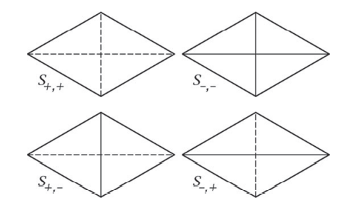
In the following figures, anti-nodal lines are indicated by dashed lines, and nodal lines by solid lines. Figure 12 displays the nodal and anti-nodal lines common to all functions in $H^{1}(\mathcal{H}) \cap \mathcal{S}{\sigma, \tau}$, where $\sigma, \tau \in{+,-}$ Denote by $R$ the rotation $R{\frac{2 \pi}{3}}$,
$$
\left{\begin{array}{l}
R=D_{2} \circ D_{1}=M_{2} \circ M_{1}=\ldots \
R^{-1}=D_{1} \circ D_{2}=M_{1} \circ M_{2}=\ldots
\end{array}\right.
$$
This is an isometry of $\mathcal{H}$, and the action $R^{*}$ of $R$ on functions is an isometry of $L^{2}(\mathcal{H})$ with respect to the $L^{2}$-inner-product.
数学代写|数论作业代写number theory代考|Symmetries and Boundary Conditions on Sub-domains
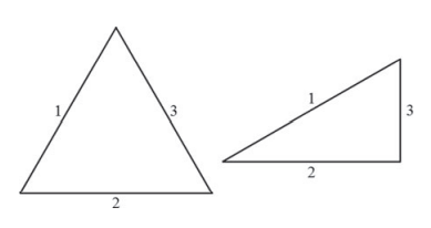
Let $\mathcal{Q}$ (resp. $\mathcal{P}$ ) denote the interior of the quadrilateral (resp. the pentagon) which appears in Fig. 14. Let $\mathcal{R}$ (resp. $\mathcal{T}{h}$ ) denote the interior of the quadrilateral (resp. of the hemiequilateral triangle) which appears in Fig. 15. Then, $\overline{\mathcal{Q}}$ (resp. $\overline{\mathcal{P}}$ ) is a fundamental domain of the action of the mirror symmetry $D{1}$ (resp. $M_{2}$ ), and $\overline{\mathcal{R}}$ is a fundamental domain for the action of the group generated by $D_{1}$ and $M_{2}$.
The boundary decompositions for the domains $\mathcal{P}, \mathcal{Q}, \mathcal{R}$, and for the hemiequilateral triangle $\mathcal{T}_{h}$, are illustrated in Figs. 14 and $15 .$
Consider the eigenvalue problem $(\mathcal{H}, \mathfrak{c})$ for the hexagon, with $\mathfrak{c} \in{\mathfrak{n}, \mathfrak{o}}$. Let $\mathcal{E}(\mu, \mathrm{c})$ be an eigenspace of $-\Delta$ for $(\mathcal{H}, \mathrm{c})$. If $\phi \in \mathcal{E}(\mu, \mathrm{c}) \cap \mathcal{S}{\sigma, \tau}$, then the restriction $\phi \mid \mathcal{R}$, of the function $\phi$ to the domain $\mathcal{R}$, is an eigenfunction of $-\Delta$ in $(\mathcal{R}, \varepsilon(\sigma) \varepsilon(\tau) \mathfrak{c})$, where $$ \varepsilon(+)=\mathfrak{n} \text { and } \varepsilon(-)=\mathfrak{o} $$ associated with the same eigenvalue $\mu$. Conversely, let $\psi$ be an eigenfunction of $-\Delta$ in $(\mathcal{R}, \mathfrak{a b c})$, associated with the eigenvalue $\mu$, where $\mathfrak{c}$ is the given boundary condition on $\partial \mathcal{H}$, and $\mathfrak{a}, \mathfrak{b} \in{\mathfrak{d}, \mathfrak{n}}$ are boundary conditions on the sides $M{2}, D_{1}$. Extend $\psi$ to a function $\breve{\psi}$ defined on $\mathcal{H}$, by symmetry (resp. anti-symmetry) with respect to $M_{2}$, if $\mathfrak{a}=\mathfrak{n}$ (resp. if $\mathfrak{a}=\mathfrak{d}$ ), and by symmetry (resp. anti-symmetry) with respect to $D_{1}$, if $\mathfrak{b}=\mathfrak{n}$ (resp. if $\mathfrak{b}=\mathfrak{d}$ ). Then, the function $\tilde{\psi}$ is an eigenfunction of $-\Delta$ for $(\mathcal{H}, \boldsymbol{c})$, associated with the eigenvalue $\mu$, and belongs to $\mathcal{S}_{\sigma, \tau}$ with $\varepsilon(\sigma)=\mathfrak{a}$ and $\varepsilon(\tau)=\mathfrak{b}$.
数学代写|数论作业代写number theory代考|Numerical Computations
Numerical approximations for the Dirichlet eigenvalues of the regular hexagon have been obtained by several authors, see for example $[5,13,16]$, or the recent paper [17].
The main idea, in order to make the identification of multiple Dirichlet eigenvalues of $\mathcal{H}$ easier, is to take the symmetries of $\mathcal{H}$ (see Sect. 3.2) into account from the start. For this purpose, one computes the eigenvalues of the domains $\mathcal{R}$ and $\mathcal{T}_{h}$, for mixed boundary conditions $\mathfrak{a} \mathfrak{b} \mathfrak{o}$, with $\mathfrak{a}, \mathfrak{b} \in{\mathfrak{d}, \mathfrak{n}}$.
Table 8 displays the first four eigenvalues of $(\mathcal{R}, \mathfrak{a} \mathfrak{b})$, as computed with MATLAB, and contains some useful relations between these eigenvalues.
Remark 3.7 The eigenvalues in Table 8 are partially ordered ‘vertically’. Indeed, for $i \geq 1$, we have the strict inequalities,
$$
\left{\begin{array}{l}
\mu_{i}(\mathcal{R}, \mathfrak{n n d})<\mu_{i}(\mathcal{R}, \mathfrak{d} \mathfrak{D} \mathfrak{J})<\mu_{i}(\mathcal{R}, \mathfrak{J} \mathfrak{J}) \
\mu_{i}\left(\mathcal{R}, \mathfrak{n n \mathfrak { J } )}<\mu_{i}(\mathcal{R}, \mathfrak{n d J})<\mu_{i}(\mathcal{R}, \mathfrak{d} \mathfrak{J})\right.
\end{array}\right.
$$
which follow from Proposition 2.2, see [22, Proposition 2.3]. These inequalities are indicated in the table by the (rotated) strict inequality signs. Note that it is general not possible to compare the eigenvalues $\mu_{i}(\mathcal{R}, \mathfrak{d} \mathfrak{n d})$ and $\mu_{i}(\mathcal{R}, \mathfrak{n d} \mathfrak{J})$. This is indicated in the table by the black question marks.
Table 9 displays some eigenvalues of $\left(\mathcal{T}_{h}, \mathfrak{a} \mathfrak{b} \mathfrak{d}\right)$, for $\mathfrak{a}, \mathfrak{b} \in{\mathfrak{d}, \mathfrak{n}}$. The lower bound in the second line follows from Dirichlet monotonicity (see Sect. 3.3.2). In the third line, we have used the fact due to Pólya (see [19]) that the first Dirichlet eigenvalue of a kite-shape is bounded from below by the first Dirichlet eigenvalue of a square with the same area. In the last two lines, the eigenvalues are known explicitly.
数论作业代写
数学代写|数论作业代写number theory代考|Symmetries and Spectra
让H表示正六边形的内部,中心在原点,边为单位长度。对角线D一世,一世=1,2,3, 连接相反的顶点和中位数米j,j=1,2,3,连接对边的中点,是六边形的镜像对称线H,见图 11。
我们考虑对角线D1和米2,以及相关的镜像对称性H. 他们通勤,
米2∘D1=D1∘米2=R圆周率
因此,我们可以应用 Sect 的方法。2.1。
它遵循D1离开子空间小号米2.±全局不变的,并且米2离开子空间小号D1,±全局不变。因此,我们有以下正交分解大号2(H),
大号2(H)=小号+,+⊕⊥小号−,−⊕⊥小号+,−⊕⊥小号−,+,
在哪里
\mathcal{S}{\sigma, \tau}:=\left{\phi \in L^{2}(\mathcal{H}) \mid D{1}^{} \phi=\sigma \phi \文本 { 和 } M_{2}^{} \phi=\tau \phi\right},\mathcal{S}{\sigma, \tau}:=\left{\phi \in L^{2}(\mathcal{H}) \mid D{1}^{} \phi=\sigma \phi \文本 { 和 } M_{2}^{} \phi=\tau \phi\right},
为了σ,τ∈+,−.
类似的分解适用于 Sobolev 空间H1(H)和H01(H), 用于 Neumann (resp. Dirichlet) 特征值的变分表示
六边形的问题。由于拉普拉斯通勤与等距D1和米2, 这样的分解也适用于−Δ在H, 有边界条件b∈○,n在边界上∂H.
在下面的图中,反节点线用虚线表示,节点线用实线表示。图 12 显示了所有函数共有的节点线和反节点线H1(H)∩小号σ,τ, 在哪里σ,τ∈+,−表示为R旋转R2圆周率3,
$$
\左{
R=D2∘D1=米2∘米1=… R−1=D1∘D2=米1∘米2=…\正确的。
$$
这是等距H, 和动作R∗的R关于函数是等距的大号2(H)相对于该大号2-内积。
数学代写|数论作业代写number theory代考|Symmetries and Boundary Conditions on Sub-domains
让问(分别。磷) 表示出现在图 14 中的四边形(或五边形)的内部。让R(分别。吨H) 表示图 15 中出现的四边形(分别为半等边三角形)的内部。然后,问¯(分别。磷¯) 是镜像对称作用的基本域D1(分别。米2), 和R¯是由生成的组的动作的基本域D1和米2.
域的边界分解磷,问,R, 对于半等边三角形吨H,如图所示。14 和15.
考虑特征值问题(H,C)对于六边形,有C∈n,○. 让和(μ,C)是一个特征空间−Δ为了(H,C). 如果φ∈和(μ,C)∩小号σ,τ,那么限制φ∣R, 的函数φ到域R, 是一个特征函数−Δ在(R,e(σ)e(τ)C), 在哪里
e(+)=n 和 e(−)=○与相同的特征值相关联μ. 反之,让ψ是一个特征函数−Δ在(R,一个bC),与特征值相关联μ, 在哪里C是给定的边界条件∂H, 和一个,b∈d,n是边上的边界条件米2,D1. 延长ψ到一个函数ψ˘定义于H,通过对称性(分别是反对称)关于米2, 如果一个=n(分别如果一个=d),并通过对称(resp.反对称)相对于D1, 如果b=n(分别如果b=d)。然后,函数ψ~是一个特征函数−Δ为了(H,C),与特征值相关联μ, 并且属于小号σ,τ和e(σ)=一个和e(τ)=b.
数学代写|数论作业代写number theory代考|Numerical Computations
几位作者已经获得了正六边形的狄利克雷特征值的数值近似,例如[5,13,16],或最近的论文 [17]。
主要思想,为了使多个狄利克雷特征值的识别H更简单,就是取对称性H(参见第 3.2 节)从一开始就考虑在内。为此,计算域的特征值R和吨H, 对于混合边界条件一个b○, 和一个,b∈d,n.
表 8 显示了前四个特征值(R,一个b),用 MATLAB 计算,并且包含这些特征值之间的一些有用关系。
备注 3.7 表 8 中的特征值是部分“垂直”排序的。的确,对于一世≥1, 我们有严格的不等式,
$$
\left{
μ一世(R,nnd)<μ一世(R,dDĴ)<μ一世(R,ĴĴ) μ一世(R,nnĴ)<μ一世(R,ndĴ)<μ一世(R,dĴ)\正确的。
$$
来自命题 2.2,参见 [22,命题 2.3]。这些不等式在表中由(旋转的)严格不等式符号表示。请注意,通常无法比较特征值μ一世(R,dnd)和μ一世(R,ndĴ). 这在表格中用黑色问号表示。
表 9 显示了一些特征值(吨H,一个bd), 为了一个,b∈d,n. 第二行的下限遵循狄利克雷单调性(参见第 3.3.2 节)。在第三行中,我们使用了由于 Pólya(参见 [19])的事实,即风筝形状的第一个 Dirichlet 特征值从下方由具有相同面积的正方形的第一个 Dirichlet 特征值界定。在最后两行中,特征值是明确已知的。

统计代写请认准statistics-lab™. statistics-lab™为您的留学生涯保驾护航。
金融工程代写
金融工程是使用数学技术来解决金融问题。金融工程使用计算机科学、统计学、经济学和应用数学领域的工具和知识来解决当前的金融问题,以及设计新的和创新的金融产品。
非参数统计代写
非参数统计指的是一种统计方法,其中不假设数据来自于由少数参数决定的规定模型;这种模型的例子包括正态分布模型和线性回归模型。
广义线性模型代考
广义线性模型(GLM)归属统计学领域,是一种应用灵活的线性回归模型。该模型允许因变量的偏差分布有除了正态分布之外的其它分布。
术语 广义线性模型(GLM)通常是指给定连续和/或分类预测因素的连续响应变量的常规线性回归模型。它包括多元线性回归,以及方差分析和方差分析(仅含固定效应)。
有限元方法代写
有限元方法(FEM)是一种流行的方法,用于数值解决工程和数学建模中出现的微分方程。典型的问题领域包括结构分析、传热、流体流动、质量运输和电磁势等传统领域。
有限元是一种通用的数值方法,用于解决两个或三个空间变量的偏微分方程(即一些边界值问题)。为了解决一个问题,有限元将一个大系统细分为更小、更简单的部分,称为有限元。这是通过在空间维度上的特定空间离散化来实现的,它是通过构建对象的网格来实现的:用于求解的数值域,它有有限数量的点。边界值问题的有限元方法表述最终导致一个代数方程组。该方法在域上对未知函数进行逼近。[1] 然后将模拟这些有限元的简单方程组合成一个更大的方程系统,以模拟整个问题。然后,有限元通过变化微积分使相关的误差函数最小化来逼近一个解决方案。
tatistics-lab作为专业的留学生服务机构,多年来已为美国、英国、加拿大、澳洲等留学热门地的学生提供专业的学术服务,包括但不限于Essay代写,Assignment代写,Dissertation代写,Report代写,小组作业代写,Proposal代写,Paper代写,Presentation代写,计算机作业代写,论文修改和润色,网课代做,exam代考等等。写作范围涵盖高中,本科,研究生等海外留学全阶段,辐射金融,经济学,会计学,审计学,管理学等全球99%专业科目。写作团队既有专业英语母语作者,也有海外名校硕博留学生,每位写作老师都拥有过硬的语言能力,专业的学科背景和学术写作经验。我们承诺100%原创,100%专业,100%准时,100%满意。
随机分析代写
随机微积分是数学的一个分支,对随机过程进行操作。它允许为随机过程的积分定义一个关于随机过程的一致的积分理论。这个领域是由日本数学家伊藤清在第二次世界大战期间创建并开始的。
时间序列分析代写
随机过程,是依赖于参数的一组随机变量的全体,参数通常是时间。 随机变量是随机现象的数量表现,其时间序列是一组按照时间发生先后顺序进行排列的数据点序列。通常一组时间序列的时间间隔为一恒定值(如1秒,5分钟,12小时,7天,1年),因此时间序列可以作为离散时间数据进行分析处理。研究时间序列数据的意义在于现实中,往往需要研究某个事物其随时间发展变化的规律。这就需要通过研究该事物过去发展的历史记录,以得到其自身发展的规律。
回归分析代写
多元回归分析渐进(Multiple Regression Analysis Asymptotics)属于计量经济学领域,主要是一种数学上的统计分析方法,可以分析复杂情况下各影响因素的数学关系,在自然科学、社会和经济学等多个领域内应用广泛。
MATLAB代写
MATLAB 是一种用于技术计算的高性能语言。它将计算、可视化和编程集成在一个易于使用的环境中,其中问题和解决方案以熟悉的数学符号表示。典型用途包括:数学和计算算法开发建模、仿真和原型制作数据分析、探索和可视化科学和工程图形应用程序开发,包括图形用户界面构建MATLAB 是一个交互式系统,其基本数据元素是一个不需要维度的数组。这使您可以解决许多技术计算问题,尤其是那些具有矩阵和向量公式的问题,而只需用 C 或 Fortran 等标量非交互式语言编写程序所需的时间的一小部分。MATLAB 名称代表矩阵实验室。MATLAB 最初的编写目的是提供对由 LINPACK 和 EISPACK 项目开发的矩阵软件的轻松访问,这两个项目共同代表了矩阵计算软件的最新技术。MATLAB 经过多年的发展,得到了许多用户的投入。在大学环境中,它是数学、工程和科学入门和高级课程的标准教学工具。在工业领域,MATLAB 是高效研究、开发和分析的首选工具。MATLAB 具有一系列称为工具箱的特定于应用程序的解决方案。对于大多数 MATLAB 用户来说非常重要,工具箱允许您学习和应用专业技术。工具箱是 MATLAB 函数(M 文件)的综合集合,可扩展 MATLAB 环境以解决特定类别的问题。可用工具箱的领域包括信号处理、控制系统、神经网络、模糊逻辑、小波、仿真等。