如果你也在 怎样代写深度学习deep learning这个学科遇到相关的难题,请随时右上角联系我们的24/7代写客服。
深度学习是机器学习的一个子集,它本质上是一个具有三层或更多层的神经网络。这些神经网络试图模拟人脑的行为–尽管远未达到与之匹配的能力–允许它从大量数据中 “学习”。
statistics-lab™ 为您的留学生涯保驾护航 在代写深度学习deep learning方面已经树立了自己的口碑, 保证靠谱, 高质且原创的统计Statistics代写服务。我们的专家在代写深度学习deep learning代写方面经验极为丰富,各种代写深度学习deep learning相关的作业也就用不着说。
我们提供的深度学习deep learning及其相关学科的代写,服务范围广, 其中包括但不限于:
- Statistical Inference 统计推断
- Statistical Computing 统计计算
- Advanced Probability Theory 高等概率论
- Advanced Mathematical Statistics 高等数理统计学
- (Generalized) Linear Models 广义线性模型
- Statistical Machine Learning 统计机器学习
- Longitudinal Data Analysis 纵向数据分析
- Foundations of Data Science 数据科学基础
机器学习代写|深度学习project代写deep learning代考|Following metrics are used for evaluation
Accuracy: It is defined as the percentage of correct predictions made by a classifier compared to the actual value of the label. It can also be defined as the average number of correct tests in all tests [13]. To calculate accuracy, we use the equation:
$$
\text { Accuracy }=(T N+T P) /(T N+T P+F N+F P) .
$$
Here, TP, TN, FP, and FN mean true positives, false negatives, false positives, and false negatives. True positive is a condition where if the class label of a record in a dataset is positive, the classifier predicts the same for that particular record. Similarly, a true negative is a condition where if the class label of a record in a dataset is negative, the classifier predicts the same for that particular record. False-positive is a condition where the class label of a record in a dataset is negative, but the classifier
predicts the class label as positive. Similarly, a false negative is a condition where the class label of a record in a dataset is positive. Still, the classifier predicts the class label as negative for that record [13].
Sensitivity: It is defined as the percentage of true positives identified by the classifier while testing. To calculate it, we use the equation:
Sensitivity $=(T P) /(T P+F N) .$
Specificity: It is defined as the percentage of true negatives which are rightly identified by the classifier during testing. To calculate it we use the equation:
$$
\text { Specificity }=(T N) /(T N+F P) .
$$
机器学习代写|深度学习project代写deep learning代考|Databases Available
Although several databases of fundus images are available publicly, the creation of quality retinal image databases is still in progress to train deep neural networks.
- DRIVE [14] (Digital Retinal Image for vessel Extraction) – This database contains 40 images collected from 400 samples of age 25 to 90 in the Netherland. Out of 40,7 shows mild DR, whereas others are normal. Each set, i.e., training and testing, includes 20 images of different patients. For every image, manual segmentation known as truths or gold standards of blood vessels is provided.
- STARE [15] (Structured Analysis of Retina) – This database contains 20 retinal fundus images taken using a fundus camera. Datasets are divided into two classes or categories, one contains normal images, and the other includes images with various lesions. CHASE [16] – contains 28 images of $1280 * 960$ pixels, taken from multi-ethnic children in England.
- Messidor and Messidor-2 [17] – These databases contain 1200 and 1748 images of the retina, respectively, taken from both eyes. Messidor- 2 is an extension of the Messidor database taken from 874 samples.
- EyePACS-1 [18] – This database contains macula-centred images of 9963 subjects taken from different cameras in May-October 2015 at EyePACS screening sites.
- APTOS [19] (Asia Pacific Tele-Ophthalmology Society) contains 3662 training images and 1928 testing images. Images are available with the ground truths classified based on severity of DR rating on a scale of 0 to 4 .
- Kaggle [20] – contains 88,702 images of the retina with different resolutions and are classified into 5 DR stages. Many images are of bad quality, and also some of the ground truths have incorrect labelling.
- IDRID [21] (Indian Diabetic Retinopathy Image Dataset) contains 516 retinal fundus images captured by a retinal specialist at an Eye Clinic located in Nanded, Maharashtra, India.
- DIARETDBI [22] contains 89 retinal fundus images of size $1500^{*} 1152$ pixels, including 5 normal images and all other 84 DR images.
- $\quad D D R[23]$ (Diagnosis of Diabetic Retinopathy) – contains 13,637 retinal fundus images showing five stages of DR. From the dataset, 757 images show DR lesions.
- Others like E-ophtha [24], HRF [25], ROC [26], and DR2 [27] etc.
机器学习代写|深度学习project代写deep learning代考|Process of Detection of DR Using Deep Learning
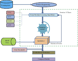
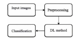
There are various numbers of supervised learning methods and unsupervised learning methods available for detecting Diabetic Retinopathy. Deep learning is one technique widely used in medical imaging applications like image classification, image segmentation, image retrieval, image detection, and registration of images. For the detection and classification of diabetic retinopathy, Deep Learning techniques or deep neural networks have been widely used. Deep neural networks produce outstanding results in the removal of default features and isolation. Unlike machine learning methods, the performance of deep learning methods increases with an increase in the number of training datasets because of an increase in learned features. There is a various number of deep neural networks like CNN (Convolutional Neural Network), RNN (Recurrent Neural Network), LSTM (Long Short Term Memory), GRU (Gated Recurrent Unit), Autoencoders, RBM (Restricted Boltzmann Machine), DBN (Deep Belief Network), DSN (Deep Stacking Network), Self-Organizing Maps, etc. Still, CNN has been widely used in medical imaging and is highly effective [11]. Deep networks are much more powerful by using strategies such as the dropout function that helps the network produce relevant results even when few features are missing in the test dataset. In addition, ReLUs (Direct Line Units) function is used as a transfer function in CNNs that helps in effective training as they do not disappear too much like the sigmoid function and tangent function used by standard ANNs. The basic architecture of CNN is that it works in different layers like Convolutional layers, pooling layers, fully connected layers, Dropout, and Activation function at last. In the convolution layer, different types of filters are used to extract features from the image. The subsampling (or pooling) layer acts as feature selection and makes the network potent to changes in size and orientation of the image. Average pooling and max pooling are mostly used in the pooling layer. A fully connected layer is used to define the whole input image. Several pretrained CNN architectures are present at the moment on ImageNet, such as LeNet, AlexNet, VGG, ResNet, GoogleNet, and more.

深度学习代写
机器学习代写|深度学习project代写deep learning代考|Following metrics are used for evaluation
准确度:定义为分类器做出的正确预测与标签实际值相比的百分比。它也可以定义为所有测试中正确测试的平均数量[13]。为了计算准确性,我们使用以下等式:
准确性 =(吨ñ+吨磷)/(吨ñ+吨磷+Fñ+F磷).
这里,TP、TN、FP 和 FN 表示真阳性、假阴性、假阳性和假阴性。真阳性是这样一种情况,如果数据集中记录的类标签为阳性,分类器对该特定记录的预测结果相同。类似地,真正的否定是这样一种情况,如果数据集中记录的类标签为负,分类器对该特定记录的预测结果相同。假阳性是数据集中记录的类标签为负的情况,但分类器
预测类标签为正。同样,假阴性是数据集中记录的类标签为正的情况。尽管如此,分类器仍将类标签预测为该记录的负数 [13]。
灵敏度:定义为测试时分类器识别的真阳性的百分比。为了计算它,我们使用以下公式:
灵敏度=(吨磷)/(吨磷+Fñ).
特异性:定义为在测试期间由分类器正确识别的真阴性的百分比。为了计算它,我们使用以下等式:
特异性 =(吨ñ)/(吨ñ+F磷).
机器学习代写|深度学习project代写deep learning代考|Databases Available
尽管有几个眼底图像数据库是公开可用的,但高质量视网膜图像数据库的创建仍在进行中,以训练深度神经网络。
- DRIVE [14](用于血管提取的数字视网膜图像)——该数据库包含从荷兰 25 至 90 岁的 400 个样本中收集的 40 张图像。在 40,7 中显示轻度 DR,而其他则正常。每组,即训练和测试,包括20张不同患者的图像。对于每张图像,都提供了称为血管真相或黄金标准的手动分割。
- STARE [15](视网膜结构分析)——该数据库包含 20 张使用眼底照相机拍摄的视网膜眼底图像。数据集分为两类或类别,一类包含正常图像,另一类包含具有各种病变的图像。CHASE [16] – 包含 28 张图片1280∗960像素,取自英格兰的多种族儿童。
- Messidor 和 Messidor-2 [17] – 这些数据库分别包含 1200 和 1748 张从双眼拍摄的视网膜图像。Messidor-2 是从 874 个样本中提取的 Messidor 数据库的扩展。
- EyePACS-1 [18] – 该数据库包含 2015 年 5 月至 2015 年 10 月在 EyePACS 筛查站点从不同相机拍摄的 9963 名受试者的黄斑中心图像。
- APTOS [19](亚太远程眼科学会)包含 3662 张训练图像和 1928 张测试图像。图像提供了根据 DR 等级的严重程度分类的基本事实,范围为 0 到 4。
- Kaggle [20] – 包含 88,702 张不同分辨率的视网膜图像,分为 5 个 DR 阶段。许多图像质量很差,而且一些基本事实的标签也不正确。
- IDRID [21](印度糖尿病视网膜病变图像数据集)包含 516 张视网膜眼底图像,由位于印度马哈拉施特拉邦南德的一家眼科诊所的视网膜专家拍摄。
- DIARETDBI [22] 包含 89 个大小的视网膜眼底图像1500∗1152像素,包括 5 个正常图像和所有其他 84 个 DR 图像。
- DDR[23](糖尿病视网膜病变的诊断)——包含 13,637 张视网膜眼底图像,显示 DR 的五个阶段。从数据集中,757 张图像显示 DR 病变。
- 其他如 E-ophtha [24]、HRF [25]、ROC [26] 和 DR2 [27] 等。
机器学习代写|深度学习project代写deep learning代考|Process of Detection of DR Using Deep Learning
有多种监督学习方法和无监督学习方法可用于检测糖尿病视网膜病变。深度学习是一种广泛用于医学成像应用的技术,如图像分类、图像分割、图像检索、图像检测和图像配准。对于糖尿病视网膜病变的检测和分类,深度学习技术或深度神经网络已被广泛使用。深度神经网络在去除默认特征和隔离方面产生了出色的效果。与机器学习方法不同,深度学习方法的性能随着训练数据集数量的增加而增加,因为学习特征的增加。有多种深度神经网络,如 CNN(卷积神经网络)、RNN(循环神经网络)、LSTM (Long Short Term Memory)、GRU (Gated Recurrent Unit)、Autoencoders、RBM (Restricted Boltzmann Machine)、DBN (Deep Belief Network)、DSN (Deep Stacking Network)、Self-Organizing Maps 等。广泛用于医学成像并且非常有效[11]。通过使用诸如 dropout 函数之类的策略,即使在测试数据集中缺少很少的特征时,深度网络也能帮助网络产生相关结果。此外,ReLU(直线单元)函数用作 CNN 中的传递函数,有助于有效训练,因为它们不会像标准 ANN 使用的 sigmoid 函数和切线函数那样消失太多。CNN 的基本架构是它在不同的层中工作,例如卷积层、池化层、全连接层、Dropout、最后是激活函数。在卷积层中,使用不同类型的过滤器从图像中提取特征。二次采样(或池化)层充当特征选择,使网络能够有效地改变图像的大小和方向。池化层主要使用平均池化和最大池化。全连接层用于定义整个输入图像。目前 ImageNet 上有几种预训练的 CNN 架构,例如 LeNet、AlexNet、VGG、ResNet、GoogleNet 等。全连接层用于定义整个输入图像。目前 ImageNet 上有几种预训练的 CNN 架构,例如 LeNet、AlexNet、VGG、ResNet、GoogleNet 等。全连接层用于定义整个输入图像。目前 ImageNet 上有几种预训练的 CNN 架构,例如 LeNet、AlexNet、VGG、ResNet、GoogleNet 等。

统计代写请认准statistics-lab™. statistics-lab™为您的留学生涯保驾护航。
金融工程代写
金融工程是使用数学技术来解决金融问题。金融工程使用计算机科学、统计学、经济学和应用数学领域的工具和知识来解决当前的金融问题,以及设计新的和创新的金融产品。
非参数统计代写
非参数统计指的是一种统计方法,其中不假设数据来自于由少数参数决定的规定模型;这种模型的例子包括正态分布模型和线性回归模型。
广义线性模型代考
广义线性模型(GLM)归属统计学领域,是一种应用灵活的线性回归模型。该模型允许因变量的偏差分布有除了正态分布之外的其它分布。
术语 广义线性模型(GLM)通常是指给定连续和/或分类预测因素的连续响应变量的常规线性回归模型。它包括多元线性回归,以及方差分析和方差分析(仅含固定效应)。
有限元方法代写
有限元方法(FEM)是一种流行的方法,用于数值解决工程和数学建模中出现的微分方程。典型的问题领域包括结构分析、传热、流体流动、质量运输和电磁势等传统领域。
有限元是一种通用的数值方法,用于解决两个或三个空间变量的偏微分方程(即一些边界值问题)。为了解决一个问题,有限元将一个大系统细分为更小、更简单的部分,称为有限元。这是通过在空间维度上的特定空间离散化来实现的,它是通过构建对象的网格来实现的:用于求解的数值域,它有有限数量的点。边界值问题的有限元方法表述最终导致一个代数方程组。该方法在域上对未知函数进行逼近。[1] 然后将模拟这些有限元的简单方程组合成一个更大的方程系统,以模拟整个问题。然后,有限元通过变化微积分使相关的误差函数最小化来逼近一个解决方案。
tatistics-lab作为专业的留学生服务机构,多年来已为美国、英国、加拿大、澳洲等留学热门地的学生提供专业的学术服务,包括但不限于Essay代写,Assignment代写,Dissertation代写,Report代写,小组作业代写,Proposal代写,Paper代写,Presentation代写,计算机作业代写,论文修改和润色,网课代做,exam代考等等。写作范围涵盖高中,本科,研究生等海外留学全阶段,辐射金融,经济学,会计学,审计学,管理学等全球99%专业科目。写作团队既有专业英语母语作者,也有海外名校硕博留学生,每位写作老师都拥有过硬的语言能力,专业的学科背景和学术写作经验。我们承诺100%原创,100%专业,100%准时,100%满意。
随机分析代写
随机微积分是数学的一个分支,对随机过程进行操作。它允许为随机过程的积分定义一个关于随机过程的一致的积分理论。这个领域是由日本数学家伊藤清在第二次世界大战期间创建并开始的。
时间序列分析代写
随机过程,是依赖于参数的一组随机变量的全体,参数通常是时间。 随机变量是随机现象的数量表现,其时间序列是一组按照时间发生先后顺序进行排列的数据点序列。通常一组时间序列的时间间隔为一恒定值(如1秒,5分钟,12小时,7天,1年),因此时间序列可以作为离散时间数据进行分析处理。研究时间序列数据的意义在于现实中,往往需要研究某个事物其随时间发展变化的规律。这就需要通过研究该事物过去发展的历史记录,以得到其自身发展的规律。
回归分析代写
多元回归分析渐进(Multiple Regression Analysis Asymptotics)属于计量经济学领域,主要是一种数学上的统计分析方法,可以分析复杂情况下各影响因素的数学关系,在自然科学、社会和经济学等多个领域内应用广泛。
MATLAB代写
MATLAB 是一种用于技术计算的高性能语言。它将计算、可视化和编程集成在一个易于使用的环境中,其中问题和解决方案以熟悉的数学符号表示。典型用途包括:数学和计算算法开发建模、仿真和原型制作数据分析、探索和可视化科学和工程图形应用程序开发,包括图形用户界面构建MATLAB 是一个交互式系统,其基本数据元素是一个不需要维度的数组。这使您可以解决许多技术计算问题,尤其是那些具有矩阵和向量公式的问题,而只需用 C 或 Fortran 等标量非交互式语言编写程序所需的时间的一小部分。MATLAB 名称代表矩阵实验室。MATLAB 最初的编写目的是提供对由 LINPACK 和 EISPACK 项目开发的矩阵软件的轻松访问,这两个项目共同代表了矩阵计算软件的最新技术。MATLAB 经过多年的发展,得到了许多用户的投入。在大学环境中,它是数学、工程和科学入门和高级课程的标准教学工具。在工业领域,MATLAB 是高效研究、开发和分析的首选工具。MATLAB 具有一系列称为工具箱的特定于应用程序的解决方案。对于大多数 MATLAB 用户来说非常重要,工具箱允许您学习和应用专业技术。工具箱是 MATLAB 函数(M 文件)的综合集合,可扩展 MATLAB 环境以解决特定类别的问题。可用工具箱的领域包括信号处理、控制系统、神经网络、模糊逻辑、小波、仿真等。