如果你也在 怎样代写量子场论Quantum field theory这个学科遇到相关的难题,请随时右上角联系我们的24/7代写客服。
在理论物理学中,量子场论(QFT)是一个理论框架,它结合了经典场论、狭义相对论和量子力学。QFT在粒子物理学中被用来构建亚原子粒子的物理模型,在凝聚态物理学中被用来构建类粒子的模型。
statistics-lab™ 为您的留学生涯保驾护航 在代写量子场论Quantum field theory方面已经树立了自己的口碑, 保证靠谱, 高质且原创的统计Statistics代写服务。我们的专家在代写量子场论Quantum field theory代写方面经验极为丰富,各种代写量子场论Quantum field theory相关的作业也就用不着说。
我们提供的量子场论Quantum field theory及其相关学科的代写,服务范围广, 其中包括但不限于:
- Statistical Inference 统计推断
- Statistical Computing 统计计算
- Advanced Probability Theory 高等概率论
- Advanced Mathematical Statistics 高等数理统计学
- (Generalized) Linear Models 广义线性模型
- Statistical Machine Learning 统计机器学习
- Longitudinal Data Analysis 纵向数据分析
- Foundations of Data Science 数据科学基础
物理代写|量子场论代写Quantum field theory代考|Position State Space for a Particle
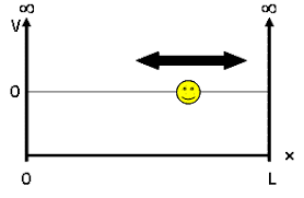
In this section we analyze how the previous machinery works to describe a very simple system, a massive point that can be located anywhere on the real line. This provides a first concrete example, and at the same time allows us to discuss the intricacies of considering infinite-dimensional state spaces. Almost nothing of what we explained in the finite-dimensional case will carry on exactly the same, but a suitable infinite-dimensional reinterpretation of the concepts will basically suffice.
The state space $\mathcal{H}$ is the space $L^{2}=L^{2}(\mathbb{R}, \mathrm{d} x)$ of complex-valued square-integrable functions ${ }^{23}$ on the real line. ${ }^{24}$ An element of $\mathcal{H}$ is thus a complex-valued function ${ }^{25} f$ on $\mathbb{R}$. The traditional terminology is to call this function the wave function. A wave function of norm 1 therefore describes the possible state of a massive point, which for simplicity we will call a particle.
The basic idea is that the position of a particle in state $f$ is not really determined, but that the function $|f|^{2}$ represents the probability density to find this particle at a given location. This statement will eventually appear as the proper interpretation of (2.6) in the present “continuous case”. To develop this idea, consider an interval $I$ of $\mathbb{R}$, and the operator $1_{I}$ defined by $1_{l}(f)(x)=f(x)$ if $x \in I$ and $1_{l}(f)(x)=0$ if $x \notin I$. This operator is bounded since $\left|1_{I}(f)\right| \leq|f|$. After we develop the right generalization of Hermitian operators in infinite dimensions, it will become apparent that this operator corresponds to an observable, and the average value of this observable on the state $f$ is
$$
\left(f, 1_{I}(f)\right)=\int_{I} \mathrm{~d} x|f(x)|^{2},
$$
which is the probability to find the particle in the set $I$. It is worth repeating the fundamental fact: When you actually measure whether the particle is in $I$ or not, you get a yes/no answer. But you are certain to find the particle in $I$ only if its state vector $f$ is an eigenvector of $1_{I}$
of eigenvalue 1, i.e. $f(x)=0$ for $x \notin I$, and you are certain not to find it in $I$ only when $f$ is an eigenvector of $1_{l}$ of eigenvalue 0 , i.e. $f(x)=0$ for $x \in I .^{26}$
In the present setting, the position of the particle is an observable so that it corresponds to a “Hermitian operator” $X$, which will be called the position operator. It is not difficult to guess what the operator $X$ should be. If indeed $|f|^{2}$ represents the probability density that the particle is at a given location, its average position is given by
$$
\int \mathrm{d} x x|f(x)|^{2}=\int \mathrm{d} x f(x)^{*}(x f(x))
$$
物理代写|量子场论代写Quantum field theory代考|Unitary Operators
We introduce now unitary operators between Hilbert spaces. It is a fundamental notion in at least two respects:
- Mathematically it provides (as explained in this section) a way to recognize whether two different models “are in fact the same”.
- Physically, countless processes are represented by unitary operators. Why this is the case is explained at the beginning of Section 2.10.
Definition 2.6.1 A linear operator $U$ between Hilbert spaces is called unitary if it is one-to-one, onto, and preserves the norm, $|U(x)|=|x|$.
Unitary transformations are in a sense the “natural class of isomorphisms between Hilbert spaces”. The “polarization identity” $|x+y|^{2}=|x|^{2}+|y|^{2}+2 \operatorname{Re}(x, y)$ shows that a unitary operator preserves the inner product, ${ }^{38}$
$$
(U(x), U(y))=(x, y) .
$$
It is almost obvious that the set $\mathcal{U}(\mathcal{H})$ of unitary operators on a Hilbert space $\mathcal{H}$ forms a group.
Next we reformulate the condition that an operator on a Hilbert space $\mathcal{H}$ is unitary using the notion of adjoint operator. As already noted, for a bounded operator $A$ one has $\mathcal{D}(A)=$ $\mathcal{D}\left(A^{\dagger}\right)=\mathcal{H}$ and
$$
\forall x, y \in \mathcal{H} ;\left(A^{\dagger}(x), y\right)=(x, A(y)) \text {. }
$$
A unitary operator on a Hilbert space is bounded, so its adjoint is defined everywhere. Furthermore by $(2.21)$ one has $\left(U^{\dagger} U(x), y\right)=(U(x), U(y))$ and $(2.20)$ is equivalent to
$U^{\dagger} U=1$. Consequently, an operator on a complex Hilbert space is unitary if and only if it is invertible and
$$
U^{-1}=U^{\dagger}
$$
Thus a unitary operator also satisfies $U U^{\dagger}=1$.
The following trivial fact is stressed because of its considerable importance.
物理代写|量子场论代写Quantum field theory代考|Momentum State Space for a Particle
To put the ideas of the previous section to use we go back to the model of a massive particle on the line which we studied in Section $2.5$. Let us consider $\mathcal{H}^{\prime}=L^{2}(\mathbb{R}, \mathrm{d} p /(2 \pi h))$, where the notation $\mathrm{d} p /(2 \pi \hbar)$ means that we include the factor $1 /(2 \pi \hbar)$ whenever we integrate in p. Consider the Fourier transform $U: f \mapsto \hat{f}$ of $(1.30)$ from $\mathcal{H}$ to $\mathcal{H}^{\prime}$. It is a unitary operator since it preserves the scalar product by (1.32) and since it has an inverse, the inverse Fourier transform $\varphi \mapsto \check{\varphi}$. The state which was represented by $f \in \mathcal{H}$ is now represented by $\varphi=\hat{f} \in \mathcal{H}^{\prime}$. As in Lemma 2.6.2 the Fourier transform $U$ transports an operator $A$ on $\mathcal{H}$ to the operator $A^{\prime}=U A U^{-1}$ on $\mathcal{H}^{\prime}$ given by $A^{\prime}(\varphi)=\widehat{A(\breve{\varphi})}$. Using (1.33) for $f=\breve{\varphi}$ yields (provided $\varphi$ is well behaved)
$$
P^{\prime}(\varphi)(p)=p \varphi(p)
$$
and, similarly,
$$
X^{\prime}(\varphi)=\mathrm{i} \hbar \frac{\mathrm{d} \varphi}{\mathrm{d} p} .
$$
(The plus sign here is not surprising since (2.19) implies that $\left[X^{\prime}, P^{\prime}\right]=\mathrm{i} \hbar 1$.) It is now the momentum operator which looks simple and the position operator which looks complicated. Just as in position state space $|f|^{2}$ represented the probability density of the location of the particle in state $f$, we can now argue that $|\varphi|^{2}$ represents the probability density of the momentum of the particle (when the basic measure is $\mathrm{d} p / 2 \pi h$ ). For this reason we will call this space $\mathcal{H}^{\prime}$ the momentum state space. Taking the Fourier transform is the standard way to analyze a wave. Thus it can be said that using momentum state space amounts to thinking of a particle as wave. This is the wave-particle duality. ${ }^{39}$
量子场论代考
物理代写|量子场论代写Quantum field theory代考|Position State Space for a Particle
在本节中,我们将分析以前的机器是如何工作的,以描述一个非常简单的系统,一个可以位于实线上任何位置的巨大点。这提供了第一个具体示例,同时允许我们讨论考虑无限维状态空间的复杂性。我们在有限维情况下解释的内容几乎没有完全相同的情况,但对概念进行适当的无限维重新解释基本上就足够了。
状态空间H是空间大号2=大号2(R,dX)复值平方可积函数23在实线上。24一个元素H因此是复值函数25F上R. 传统的术语是将此函数称为波函数。因此,范数为 1 的波函数描述了一个大质量点的可能状态,为简单起见,我们将其称为粒子。
基本思想是粒子在状态中的位置F不是真的确定,而是函数|F|2表示在给定位置找到该粒子的概率密度。该陈述最终将作为当前“连续案例”中(2.6)的正确解释出现。为了发展这个想法,考虑一个区间我的R, 和运算符1我被定义为1l(F)(X)=F(X)如果X∈我和1l(F)(X)=0如果X∉我. 这个算子是有界的,因为|1我(F)|≤|F|. 在我们开发出无限维 Hermitian 算子的正确推广之后,很明显,这个算子对应于一个可观察的,并且这个可观察的在状态上的平均值F是
(F,1我(F))=∫我 dX|F(X)|2,
这是在集合中找到粒子的概率我. 值得重复一个基本事实:当你实际测量粒子是否在我与否,你会得到一个是/否的答案。但你肯定会在我只有当它的状态向量F是一个特征向量1我
特征值 1,即F(X)=0为了X∉我, 你肯定不会在我只有当F是一个特征向量1l特征值 0 ,即F(X)=0为了X∈我.26
在当前设置中,粒子的位置是可观察的,因此它对应于“厄米算子”X,这将被称为位置运算符。不难猜出运营商是什么X应该。如果确实|F|2表示粒子在给定位置的概率密度,其平均位置由下式给出
∫dXX|F(X)|2=∫dXF(X)∗(XF(X))
物理代写|量子场论代写Quantum field theory代考|Unitary Operators
我们现在介绍希尔伯特空间之间的酉算子。它至少在两个方面是一个基本概念:
- 从数学上讲,它提供了(如本节所述)一种识别两个不同模型是否“实际上相同”的方法。
- 在物理上,无数的过程由单一运算符表示。为什么会出现这种情况在 2.10 节的开头进行了解释。
定义 2.6.1 线性算子在希尔伯特空间之间称为酉,如果它是一对一的,并保持范数,|在(X)|=|X|.
酉变换在某种意义上是“希尔伯特空间之间的自然类同构”。“极化身份”|X+是|2=|X|2+|是|2+2回覆(X,是)表明酉算子保留内积,38
(在(X),在(是))=(X,是).
几乎很明显,集合在(H)希尔伯特空间上的酉算子H形成一个群体。
接下来我们重新制定希尔伯特空间上的算子的条件H使用伴随算子的概念是酉的。如前所述,对于有界算子一个一个有D(一个)= D(一个†)=H和
∀X,是∈H;(一个†(X),是)=(X,一个(是)).
希尔伯特空间上的酉算子是有界的,所以它的伴随是到处定义的。此外通过(2.21)一个有(在†在(X),是)=(在(X),在(是))和(2.20)相当于
在†在=1. 因此,复希尔伯特空间上的算子是酉当且仅当它是可逆的并且
在−1=在†
因此酉算子也满足在在†=1.
强调以下琐碎的事实,因为它相当重要。
物理代写|量子场论代写Quantum field theory代考|Momentum State Space for a Particle
为了使用上一节的想法,我们回到我们在第 1 节研究的线上的大质量粒子模型2.5. 让我们考虑一下H′=大号2(R,dp/(2圆周率H)), 其中符号dp/(2圆周率⁇)意味着我们包括因素1/(2圆周率⁇)每当我们整合到 p 中时。考虑傅里叶变换在:F↦F^的(1.30)从H至H′. 它是一个酉算子,因为它保留了 (1.32) 的标量积,并且由于它具有逆傅里叶变换披↦披ˇ. 所代表的状态F∈H现在由披=F^∈H′. 如引理 2.6.2 中的傅里叶变换在运输操作员一个上H给运营商一个′=在一个在−1上H′由一个′(披)=一个(披˘)^. 使用(1.33)F=披˘产量(提供披表现良好)
磷′(披)(p)=p披(p)
同样,
X′(披)=一世⁇d披dp.
(这里的加号并不奇怪,因为(2.19)意味着[X′,磷′]=一世⁇1.) 现在是动量算子看起来很简单,而位置算子看起来很复杂。就像在位置状态空间中一样|F|2表示状态中粒子位置的概率密度F,我们现在可以说|披|2表示粒子动量的概率密度(当基本度量为dp/2圆周率H)。出于这个原因,我们将这个空间称为H′动量状态空间。傅里叶变换是分析波的标准方法。因此可以说,使用动量态空间相当于将粒子视为波。这就是波粒二象性。39

统计代写请认准statistics-lab™. statistics-lab™为您的留学生涯保驾护航。
金融工程代写
金融工程是使用数学技术来解决金融问题。金融工程使用计算机科学、统计学、经济学和应用数学领域的工具和知识来解决当前的金融问题,以及设计新的和创新的金融产品。
非参数统计代写
非参数统计指的是一种统计方法,其中不假设数据来自于由少数参数决定的规定模型;这种模型的例子包括正态分布模型和线性回归模型。
广义线性模型代考
广义线性模型(GLM)归属统计学领域,是一种应用灵活的线性回归模型。该模型允许因变量的偏差分布有除了正态分布之外的其它分布。
术语 广义线性模型(GLM)通常是指给定连续和/或分类预测因素的连续响应变量的常规线性回归模型。它包括多元线性回归,以及方差分析和方差分析(仅含固定效应)。
有限元方法代写
有限元方法(FEM)是一种流行的方法,用于数值解决工程和数学建模中出现的微分方程。典型的问题领域包括结构分析、传热、流体流动、质量运输和电磁势等传统领域。
有限元是一种通用的数值方法,用于解决两个或三个空间变量的偏微分方程(即一些边界值问题)。为了解决一个问题,有限元将一个大系统细分为更小、更简单的部分,称为有限元。这是通过在空间维度上的特定空间离散化来实现的,它是通过构建对象的网格来实现的:用于求解的数值域,它有有限数量的点。边界值问题的有限元方法表述最终导致一个代数方程组。该方法在域上对未知函数进行逼近。[1] 然后将模拟这些有限元的简单方程组合成一个更大的方程系统,以模拟整个问题。然后,有限元通过变化微积分使相关的误差函数最小化来逼近一个解决方案。
tatistics-lab作为专业的留学生服务机构,多年来已为美国、英国、加拿大、澳洲等留学热门地的学生提供专业的学术服务,包括但不限于Essay代写,Assignment代写,Dissertation代写,Report代写,小组作业代写,Proposal代写,Paper代写,Presentation代写,计算机作业代写,论文修改和润色,网课代做,exam代考等等。写作范围涵盖高中,本科,研究生等海外留学全阶段,辐射金融,经济学,会计学,审计学,管理学等全球99%专业科目。写作团队既有专业英语母语作者,也有海外名校硕博留学生,每位写作老师都拥有过硬的语言能力,专业的学科背景和学术写作经验。我们承诺100%原创,100%专业,100%准时,100%满意。
随机分析代写
随机微积分是数学的一个分支,对随机过程进行操作。它允许为随机过程的积分定义一个关于随机过程的一致的积分理论。这个领域是由日本数学家伊藤清在第二次世界大战期间创建并开始的。
时间序列分析代写
随机过程,是依赖于参数的一组随机变量的全体,参数通常是时间。 随机变量是随机现象的数量表现,其时间序列是一组按照时间发生先后顺序进行排列的数据点序列。通常一组时间序列的时间间隔为一恒定值(如1秒,5分钟,12小时,7天,1年),因此时间序列可以作为离散时间数据进行分析处理。研究时间序列数据的意义在于现实中,往往需要研究某个事物其随时间发展变化的规律。这就需要通过研究该事物过去发展的历史记录,以得到其自身发展的规律。
回归分析代写
多元回归分析渐进(Multiple Regression Analysis Asymptotics)属于计量经济学领域,主要是一种数学上的统计分析方法,可以分析复杂情况下各影响因素的数学关系,在自然科学、社会和经济学等多个领域内应用广泛。
MATLAB代写
MATLAB 是一种用于技术计算的高性能语言。它将计算、可视化和编程集成在一个易于使用的环境中,其中问题和解决方案以熟悉的数学符号表示。典型用途包括:数学和计算算法开发建模、仿真和原型制作数据分析、探索和可视化科学和工程图形应用程序开发,包括图形用户界面构建MATLAB 是一个交互式系统,其基本数据元素是一个不需要维度的数组。这使您可以解决许多技术计算问题,尤其是那些具有矩阵和向量公式的问题,而只需用 C 或 Fortran 等标量非交互式语言编写程序所需的时间的一小部分。MATLAB 名称代表矩阵实验室。MATLAB 最初的编写目的是提供对由 LINPACK 和 EISPACK 项目开发的矩阵软件的轻松访问,这两个项目共同代表了矩阵计算软件的最新技术。MATLAB 经过多年的发展,得到了许多用户的投入。在大学环境中,它是数学、工程和科学入门和高级课程的标准教学工具。在工业领域,MATLAB 是高效研究、开发和分析的首选工具。MATLAB 具有一系列称为工具箱的特定于应用程序的解决方案。对于大多数 MATLAB 用户来说非常重要,工具箱允许您学习和应用专业技术。工具箱是 MATLAB 函数(M 文件)的综合集合,可扩展 MATLAB 环境以解决特定类别的问题。可用工具箱的领域包括信号处理、控制系统、神经网络、模糊逻辑、小波、仿真等。