如果你也在 怎样代写决策与风险decision and risk这个学科遇到相关的难题,请随时右上角联系我们的24/7代写客服。
决策与风险分析帮助组织在存在风险和不确定性的情况下做出决策,使其效用最大化。
风险决策。一个组织的领导层决定接受一个具有特定风险功能的选项,而不是另一个,或者是不采取任何行动。我认为,任何有价值的组织的主管领导都可以在适当的级别上做出这样的决定。
这个术语是在备选方案之间做出决定的简称,其中至少有一个方案有损失的概率。(通常在网络风险中,我们关注的是损失,但所有的想法都自然地延伸到上升或机会风险。很少有人和更少的组织会在没有预期利益的情况下承担风险,即使只是避免成本)。
损失大小的概率分布,在某个规定的时间段,如一年。这就是我认为大多数人在谈论某物的 “风险 “时的真正含义。
statistics-lab™ 为您的留学生涯保驾护航 在代写决策与风险decision and risk方面已经树立了自己的口碑, 保证靠谱, 高质且原创的统计Statistics代写服务。我们的专家在代写决策与风险decision and risk方面经验极为丰富,各种代写决策与风险decision and risk相关的作业也就用不着说。
我们提供的决策与风险decision and risk及其相关学科的代写,服务范围广, 其中包括但不限于:
- Statistical Inference 统计推断
- Statistical Computing 统计计算
- Advanced Probability Theory 高等楖率论
- Advanced Mathematical Statistics 高等数理统计学
- (Generalized) Linear Models 广义线性模型
- Statistical Machine Learning 统计机器学习
- Longitudinal Data Analysis 纵向数据分析
- Foundations of Data Science 数据科学基础
统计代写|决策与风险作业代写decision and risk代考|A Simple Inventory Model
The simple model that we introduce below is based on the model proposed in Muñoz and Muñoz (2011) to forecast the demand of items with sporadic demand, and is inspired in the ideas of Kalchsmidth et al. (2006), where they suggest the use of forecasting techniques that take into account not only the time series, but also the structure of the process that generates the demand (non-systematic variability). In what follows we will refer to this model as Model $1 .$
Let us suppose that a seller uses a $(Q, R$ ) policy (see, e.g., Nahmias 2013 ) to order the supply of a certain product, i.e., when the inventory level reaches the reorder point $(R)$, a quantity $Q$ is ordered. If an order is placed at time $t=0$ and $L$ is the delay, then the demand for the product during the delay is
$$
W_{1}=\left{\begin{array}{cc}
\sum_{i=1}^{N(L)} U_{i}, & N(L)>0 \
0, & \text { otherwise }
\end{array}\right.
$$
where, for $t \geq 0, N(t)$ is the number of clients that arrived up to time t, and for $i=1,2, \ldots, U_{i}$ is the demand for client $i$. We assume that $U_{1}, U_{2}, \ldots$ are i.i.d. random variables and are also independent of the stochastic process ${N(t): t \geq 0}$. In order to obtain analytical results for some of our performance measures, we also assume that ${N(t): t \geq 0}$ is a Poisson process with rate $\Theta_{0}$.
Under our assumptions, we can define the following parameters that represent important properties for the policy $(Q, R)$ (for details on the derivation of the analytical expressions see Muñoz et al. 2013).
The expected demand is an important measure to forecast demand $W_{1}$, and is defined by
$$
\mu_{W}=E\left[W_{1}\right]=\Theta_{0} L \mu_{U}
$$
where $E[X]$ denotes the expected value of a random variable $X$, and $\mu_{U}=E\left[U_{1}\right]$.
The variance of demand $W_{1}$ is an important measure for the magnitude of the uncertainty on the forecast of demand $W_{1}$, and is defined by
$$
\sigma_{W}^{2}=E\left[W_{1}^{2}\right]-E\left[W_{1}\right]^{2}=\Theta_{0} L\left(\mu_{U}^{2}+\sigma_{U}^{2}\right)
$$
where $\mu_{U}^{2}=E\left[U_{1}\right]^{2}, \sigma_{U}^{2}=E\left[U_{1}^{2}\right]-\mu_{U^{*}}^{2}$
Given a value $R$ for the reorder point, an important risk measure is the probability of no stockout (called type-l service level), and is defined by
$$
\alpha_{1}(R)=P\left[W_{1} \leq R\right]=E\left[I\left(W_{1} \leq R\right)\right]
$$
where, for any event $A, I(A)$ denotes the indicator random variable that takes a value of 1 if event $A$ occurs and zero otherwise.
Given a value $0<\alpha<1$, the type-1 reorder point is a value for the reorder point that provides an approximate type-1 service level of $\alpha$, and is defined by
$$
r_{1}(\alpha)=\inf \left{R \geq 0: \alpha_{1}(R) \geq \alpha\right}
$$
where $\alpha_{1}(R)$ is defined in (6.5).
Similarly, given a value $R$ for the reorder point, another important risk measure is the proportion of demand that is met from stock (called type-2 service level or fill
rate), and is defined by
$$
\alpha_{2}(R)=1-\frac{E\left[\left(W_{1}-R\right) I\left(W_{1}>R\right)\right]}{Q}
$$
and given a value $0<\alpha<1$, the type-2 reorder point is a value for the reorder point that provides an approximate type- 2 service level of $\alpha$, and is defined by
$$
r_{2}(\alpha)=\inf \left{R \geq 0: \alpha_{2}(R) \geq \alpha\right}
$$
where $\alpha_{2}(R)$ is defined in $(6.7)$.
In the next sections, we show how to estimate the measures of risk defined by Eqs. (6.3) through (6.6) from the output of a simulation, and remark that Model 1 , as defined in (6.1), is a very simple model just to verify (using simulation) that we are proposing valid estimation procedures that may be applied to a complex model, for which we would not have analytical solutions.
统计代写|决策与风险作业代写decision and risk代考|Properties of a Good Estimator
In order to discuss the main properties that a good simulation-based estimator must satisfy, we use the concept of weak converge of random variables. We say that a sequence of random variables $X_{1}, X_{2}, \ldots$ converge weakly to a random variable $X$ (and denote $X_{m} \Rightarrow X$, as $m \rightarrow \infty$ ), if $\lim {m \rightarrow \infty} F{X_{m}}(x)=F_{X}(x)$, at any point $x$ where $F$ is continuous, where $F_{X_{m}}$ and $F_{X}$ denote the c.d.f. of $X_{m}$ and $X$, respectively (see, e.g., Chung 2000 ). Note that $X$ can also be a constant $(M)$, on which case $X$ is simply the random variable that takes the value of $M$ with probability 1 .
A first property that a good estimator must satisfy is consistency. We say that the estimator $T\left(F_{m}\right)$, where $F_{m}$ is defined in (6.1) is consistent if
$$
T\left(F_{m}\right) \Rightarrow T(F)
$$
as $m \rightarrow \infty$. Note that consistency means that the estimator $T\left(F_{m}\right)$ approaches the parameter $T(F)$ as the sample size $m$ increases, and this is a required property since we do not want the estimator to converge to a different value (or not to converge at all).
In order to assess the accuracy of a consistent estimator $T\left(F_{m}\right)$, we usually verify if a Central Limit Theorem (CLT) in the form of
$$
\frac{\sqrt{m}\left(T\left(F_{m}\right)-T(F)\right)}{\sigma_{T}} \Rightarrow N(0,1)
$$
as $m \rightarrow \infty$ is satisfied, on which case we may also look for a consistent estimator $\hat{\sigma}^{2}(m)$ for the asymptotic variance $\sigma_{T}^{2}$, so that if follows from $(6.10)$ and standard
properties of weak convergence (see, e.g., Serfling 2009) that
$$
\frac{\sqrt{m}\left(T\left(F_{m}\right)-T(F)\right)}{\hat{\sigma}(m)} \Rightarrow N(0,1),
$$
as $m \rightarrow \infty$, where $N(0,1)$ denotes a random variable distributed as Normal with mean 0 and variance 1 . It is worth mentioning that the CLT of (6.10) implies consistency of $T\left(F_{m}\right)$, as defined in (6.9).
A CLT in the form of $(6.11)$ is sufficient to assess the accuracy of the point estimator $T\left(F_{m}\right)$, since (6.11) implies that
$$
\lim {m \rightarrow \infty} P\left[\left|T\left(F{m}\right)-T(F)\right| \leq z_{\beta} \frac{\hat{\sigma}(m)}{\sqrt{m}}\right]=1-\beta
$$
where $z_{\beta}$ denotes the $(1-\beta / 2)$-quantile of a $N(0,1)$, which is sufficient to establish an asymptotically valid $(1-\beta) 100 \%$ confidence interval (CI) for $T(F)$ with halfwidth
$$
H W_{T}=\frac{t_{(m-1, \beta)} \hat{\sigma}(m)}{\sqrt{m}}
$$
where $t_{(m-1, \beta)}$ denotes the $(1-\beta / 2)$-quantile of a Student-t distribution with $(\mathrm{m}-$ 1) degrees of freedom. A halfwidth in the form of $(6.12)$ is the typical measure used in simulation software to assess the accuracy of $T\left(F_{m}\right)$ for the estimation of a parameter $T(F)$. Note that we are using a Student-t distribution to have a wider CI when the value of $m$ is small, and the CI is still asymptotically valid since $t_{(m-1, \beta)} \rightarrow z_{\beta}$, as $m \rightarrow \infty$. Note also from (6.12) that, to lower the value of a halfwidth (i.e., improve the accuracy of $T\left(F_{m}\right)$ ), we need to increase the sample size $m$, so that the halfwidth will be reduced approximately by half if we multiply the sample size $m$ by 4 .
统计代写|决策与风险作业代写decision and risk代考|Estimation of Expected Values
For the estimation of the expected value $T(F)=E\left[W_{1}\right]$, the point estimator $T\left(F_{m}\right)$ becomes the sample average
$$
\bar{W}(m)=\frac{\sum_{i=1}^{m} W_{i}}{m},
$$
and it is well-known from the classical CLT that the CLT (6.10) is satisfied for $T\left(F_{m}\right)=\bar{W}(m)$, and $\sigma_{T}^{2}=E\left[W_{1}^{2}\right]-E\left[W_{1}\right]^{2}$. Moreover, since $W_{1}, W_{2}, \ldots, W_{m}$ are i.i.d., it is well known that a consistent (and unbiased) estimator for $\sigma_{T}^{2}$ is
$$
S_{W}^{2}(m)=\frac{\sum_{i=1}^{m}\left(W_{i}-\bar{W}(m)\right)^{2}}{m-1}
$$
so that, it follows from (6.11) that an asymptotically valid $(1-\beta) 100 \%$ halfwidth for the expected value $\mu_{W}=E\left[W_{1}\right]$ is given by
$$
H W_{\mu_{W}}=\frac{t_{(m-1 . \beta)} S_{W}(m)}{\sqrt{m}},
$$
where $S_{W}(m)$ is defined in (6.14).
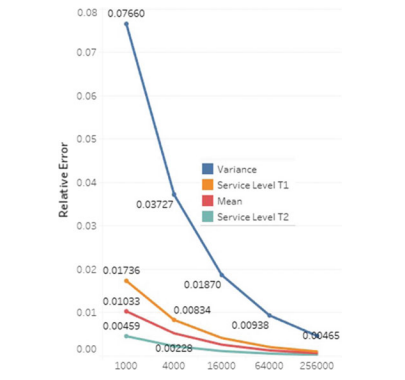
Thus, Eq. (6.13) can be used to compute a point estimator for the expected value in a transient simulation, and Eq. (6.15) allows us to compute an assessment of the accuracy of the point estimator. Note that Eqs. (6.13) and (6.15) can be applied not only to the estimation of the expected demand (6.3) in Model 1 but also for the estimation of a type-1 service level defined in (6.5) or a type- 2 service level defined in (6.7), since the service levels are also expectations, to be more precise, we can take $W_{1 i}=I\left[W_{i} \leq R\right]$ for parameter $(6.5)$ and $W_{2 i}=1-\left(W_{i}-R\right) I\left[W_{i}>R\right] / Q$ for parameter $(6.7), i=1, \ldots, m$. A $\mathrm{C}++$ code for the estimation of these risk measures using simulation output was compiled to produce a library and below we report numerical examples using this code.
决策与风险代写
统计代写|决策与风险作业代写decision and risk代考|A Simple Inventory Model
我们下面介绍的简单模型是基于 Muñoz 和 Muñoz (2011) 提出的用于预测零星需求项目需求的模型,并受到 Kalchsmidth 等人的想法的启发。(2006 年),他们建议使用预测技术,不仅要考虑时间序列,还要考虑产生需求的过程结构(非系统可变性)。在下文中,我们将这个模型称为模型1.
让我们假设卖家使用(问,R) 政策(例如,参见 Nahmias 2013 )订购某种产品的供应,即当库存水平达到再订购点时(R), 一个量问被订购。如果在某个时间下订单吨=0和大号是延迟,则延迟期间对产品的需求为
$$
W_{1}=\left{∑一世=1ñ(大号)ü一世,ñ(大号)>0 0, 除此以外 \对。
$$
在哪里,对于吨≥0,ñ(吨)是在时间 t 之前到达的客户数量,对于一世=1,2,…,ü一世是客户的需求一世. 我们假设ü1,ü2,…是独立同分布的随机变量,也独立于随机过程ñ(吨):吨≥0. 为了获得我们的一些绩效指标的分析结果,我们还假设ñ(吨):吨≥0是一个具有速率的 Poisson 过程θ0.
在我们的假设下,我们可以定义以下代表策略重要属性的参数(问,R)(有关推导解析表达式的详细信息,请参见 Muñoz 等人,2013 年)。
预期需求是预测需求的重要指标在1,并且定义为
μ在=和[在1]=θ0大号μü
在哪里和[X]表示随机变量的期望值X, 和μü=和[ü1].
需求方差在1是衡量需求预测不确定性大小的重要指标在1,并且定义为
σ在2=和[在12]−和[在1]2=θ0大号(μü2+σü2)
在哪里μü2=和[ü1]2,σü2=和[ü12]−μü∗2
给定一个值R对于再订货点,一个重要的风险度量是没有缺货的概率(称为 L 类服务水平),定义为
一种1(R)=磷[在1≤R]=和[一世(在1≤R)]
在哪里,对于任何事件一种,一世(一种)表示如果事件取值为 1 的指标随机变量一种发生,否则为零。
给定一个值0<一种<1,类型 1 再订购点是提供近似类型 1 服务水平的再订购点的值一种,并且定义为
r_{1}(\alpha)=\inf \left{R \geq 0: \alpha_{1}(R) \geq \alpha\right}r_{1}(\alpha)=\inf \left{R \geq 0: \alpha_{1}(R) \geq \alpha\right}
在哪里一种1(R)在 (6.5) 中定义。
同样,给定一个值R对于再订货点,另一个重要的风险度量是库存满足需求的比例(称为类型 2 服务水平或填充
率),并定义为
一种2(R)=1−和[(在1−R)一世(在1>R)]问
并给出一个值0<一种<1,类型 2 再订购点是提供近似类型 2 服务水平的再订购点的值一种,并且定义为
r_{2}(\alpha)=\inf \left{R \geq 0: \alpha_{2}(R) \geq \alpha\right}r_{2}(\alpha)=\inf \left{R \geq 0: \alpha_{2}(R) \geq \alpha\right}
在哪里一种2(R)定义在(6.7).
在接下来的部分中,我们将展示如何估计由方程式定义的风险度量。(6.3) 到 (6.6) 从模拟的输出,并注意模型 1,如 (6.1) 中定义的,是一个非常简单的模型,只是为了验证(使用模拟)我们提出了可以应用的有效估计程序到一个复杂的模型,我们没有分析解决方案。
统计代写|决策与风险作业代写decision and risk代考|Properties of a Good Estimator
为了讨论一个好的基于模拟的估计器必须满足的主要性质,我们使用随机变量弱收敛的概念。我们说一系列随机变量X1,X2,…弱收敛到随机变量X(并表示X米⇒X, 作为米→∞), 如果林米→∞FX米(X)=FX(X), 在任何时候X在哪里F是连续的,其中FX米和FX表示的 cdfX米和X,分别(参见,例如,Chung 2000)。注意X也可以是常数(米), 在这种情况下X只是取值的随机变量米概率为 1 。
一个好的估计器必须满足的第一个属性是一致性。我们说估计器吨(F米), 在哪里F米在 (6.1) 中定义是一致的,如果
吨(F米)⇒吨(F)
作为米→∞. 请注意,一致性意味着估计量吨(F米)逼近参数吨(F)作为样本量米增加,这是一个必需的属性,因为我们不希望估计器收敛到不同的值(或根本不收敛)。
为了评估一致估计器的准确性吨(F米), 我们通常验证一个中心极限定理 (CLT) 的形式为
米(吨(F米)−吨(F))σ吨⇒ñ(0,1)
作为米→∞满意,在这种情况下,我们也可以寻找一致的估计量σ^2(米)对于渐近方差σ吨2,所以如果从(6.10)和标准
弱收敛的特性(参见例如 Serfling 2009)
米(吨(F米)−吨(F))σ^(米)⇒ñ(0,1),
作为米→∞, 在哪里ñ(0,1)表示一个随机变量,分布为正态分布,均值为 0,方差为 1。值得一提的是,(6.10) 的 CLT 意味着吨(F米),如 (6.9) 中所定义。
形式为 CLT(6.11)足以评估点估计器的准确性吨(F米), 因为 (6.11) 意味着
林米→∞磷[|吨(F米)−吨(F)|≤和bσ^(米)米]=1−b
在哪里和b表示(1−b/2)-a的分位数ñ(0,1),这足以建立渐近有效的(1−b)100%置信区间 (CI)吨(F)半角
H在吨=吨(米−1,b)σ^(米)米
在哪里吨(米−1,b)表示(1−b/2)-Student-t 分布的分位数(米−1) 自由度。半角形式为(6.12)是模拟软件中用于评估精度的典型措施吨(F米)用于估计参数吨(F). 请注意,当值为米很小,并且 CI 仍然是渐近有效的,因为吨(米−1,b)→和b, 作为米→∞. 还要注意(6.12)中,要降低半角的值(即,提高吨(F米)),我们需要增加样本量米,因此如果我们乘以样本大小,半宽将减少大约一半米由 4 .
统计代写|决策与风险作业代写decision and risk代考|Estimation of Expected Values
用于估计期望值吨(F)=和[在1], 点估计器吨(F米)成为样本平均值
在¯(米)=∑一世=1米在一世米,
并且从经典 CLT 中众所周知,CLT (6.10) 满足吨(F米)=在¯(米), 和σ吨2=和[在12]−和[在1]2. 此外,由于在1,在2,…,在米是独立同分布的,众所周知,对于σ吨2是小号在2(米)=∑一世=1米(在一世−在¯(米))2米−1
因此,从 (6.11) 可以得出一个渐近有效的(1−b)100%期望值的半角μ在=和[在1]是(谁)给的
H在μ在=吨(米−1.b)小号在(米)米,
在哪里小号在(米)在 (6.14) 中定义。
因此,方程。(6.13)式可用于计算瞬态模拟中期望值的点估计量,方程。(6.15) 允许我们计算对点估计器准确性的评估。请注意,方程式。(6.13) 和 (6.15) 不仅可以应用于模型 1 中预期需求 (6.3) 的估计,还可以应用于 (6.5) 中定义的类型 1 服务水平或定义的类型 2 服务水平的估计在(6.7)中,由于服务水平也是期望,更准确地说,我们可以取在1一世=一世[在一世≤R]对于参数(6.5)和在2一世=1−(在一世−R)一世[在一世>R]/问对于参数(6.7),一世=1,…,米. 一种C++编译使用模拟输出估计这些风险措施的代码以生成一个库,下面我们使用此代码报告数值示例。

统计代写请认准statistics-lab™. statistics-lab™为您的留学生涯保驾护航。统计代写|python代写代考
随机过程代考
在概率论概念中,随机过程是随机变量的集合。 若一随机系统的样本点是随机函数,则称此函数为样本函数,这一随机系统全部样本函数的集合是一个随机过程。 实际应用中,样本函数的一般定义在时间域或者空间域。 随机过程的实例如股票和汇率的波动、语音信号、视频信号、体温的变化,随机运动如布朗运动、随机徘徊等等。
贝叶斯方法代考
贝叶斯统计概念及数据分析表示使用概率陈述回答有关未知参数的研究问题以及统计范式。后验分布包括关于参数的先验分布,和基于观测数据提供关于参数的信息似然模型。根据选择的先验分布和似然模型,后验分布可以解析或近似,例如,马尔科夫链蒙特卡罗 (MCMC) 方法之一。贝叶斯统计概念及数据分析使用后验分布来形成模型参数的各种摘要,包括点估计,如后验平均值、中位数、百分位数和称为可信区间的区间估计。此外,所有关于模型参数的统计检验都可以表示为基于估计后验分布的概率报表。
广义线性模型代考
广义线性模型(GLM)归属统计学领域,是一种应用灵活的线性回归模型。该模型允许因变量的偏差分布有除了正态分布之外的其它分布。
statistics-lab作为专业的留学生服务机构,多年来已为美国、英国、加拿大、澳洲等留学热门地的学生提供专业的学术服务,包括但不限于Essay代写,Assignment代写,Dissertation代写,Report代写,小组作业代写,Proposal代写,Paper代写,Presentation代写,计算机作业代写,论文修改和润色,网课代做,exam代考等等。写作范围涵盖高中,本科,研究生等海外留学全阶段,辐射金融,经济学,会计学,审计学,管理学等全球99%专业科目。写作团队既有专业英语母语作者,也有海外名校硕博留学生,每位写作老师都拥有过硬的语言能力,专业的学科背景和学术写作经验。我们承诺100%原创,100%专业,100%准时,100%满意。
机器学习代写
随着AI的大潮到来,Machine Learning逐渐成为一个新的学习热点。同时与传统CS相比,Machine Learning在其他领域也有着广泛的应用,因此这门学科成为不仅折磨CS专业同学的“小恶魔”,也是折磨生物、化学、统计等其他学科留学生的“大魔王”。学习Machine learning的一大绊脚石在于使用语言众多,跨学科范围广,所以学习起来尤其困难。但是不管你在学习Machine Learning时遇到任何难题,StudyGate专业导师团队都能为你轻松解决。
多元统计分析代考
基础数据: $N$ 个样本, $P$ 个变量数的单样本,组成的横列的数据表
变量定性: 分类和顺序;变量定量:数值
数学公式的角度分为: 因变量与自变量
时间序列分析代写
随机过程,是依赖于参数的一组随机变量的全体,参数通常是时间。 随机变量是随机现象的数量表现,其时间序列是一组按照时间发生先后顺序进行排列的数据点序列。通常一组时间序列的时间间隔为一恒定值(如1秒,5分钟,12小时,7天,1年),因此时间序列可以作为离散时间数据进行分析处理。研究时间序列数据的意义在于现实中,往往需要研究某个事物其随时间发展变化的规律。这就需要通过研究该事物过去发展的历史记录,以得到其自身发展的规律。
回归分析代写
多元回归分析渐进(Multiple Regression Analysis Asymptotics)属于计量经济学领域,主要是一种数学上的统计分析方法,可以分析复杂情况下各影响因素的数学关系,在自然科学、社会和经济学等多个领域内应用广泛。
MATLAB代写
MATLAB 是一种用于技术计算的高性能语言。它将计算、可视化和编程集成在一个易于使用的环境中,其中问题和解决方案以熟悉的数学符号表示。典型用途包括:数学和计算算法开发建模、仿真和原型制作数据分析、探索和可视化科学和工程图形应用程序开发,包括图形用户界面构建MATLAB 是一个交互式系统,其基本数据元素是一个不需要维度的数组。这使您可以解决许多技术计算问题,尤其是那些具有矩阵和向量公式的问题,而只需用 C 或 Fortran 等标量非交互式语言编写程序所需的时间的一小部分。MATLAB 名称代表矩阵实验室。MATLAB 最初的编写目的是提供对由 LINPACK 和 EISPACK 项目开发的矩阵软件的轻松访问,这两个项目共同代表了矩阵计算软件的最新技术。MATLAB 经过多年的发展,得到了许多用户的投入。在大学环境中,它是数学、工程和科学入门和高级课程的标准教学工具。在工业领域,MATLAB 是高效研究、开发和分析的首选工具。MATLAB 具有一系列称为工具箱的特定于应用程序的解决方案。对于大多数 MATLAB 用户来说非常重要,工具箱允许您学习和应用专业技术。工具箱是 MATLAB 函数(M 文件)的综合集合,可扩展 MATLAB 环境以解决特定类别的问题。可用工具箱的领域包括信号处理、控制系统、神经网络、模糊逻辑、小波、仿真等。