如果你也在 怎样代写工程统计engineering statistics这个学科遇到相关的难题,请随时右上角联系我们的24/7代写客服。
工程统计结合了工程和统计,使用科学方法分析数据。工程统计涉及有关制造过程的数据,如:部件尺寸、公差、材料类型和制造过程控制。
statistics-lab™ 为您的留学生涯保驾护航 在代写工程统计engineering statistics方面已经树立了自己的口碑, 保证靠谱, 高质且原创的统计Statistics代写服务。我们的专家在代写工程统计engineering statistics代写方面经验极为丰富,各种代写工程统计engineering statistics相关的作业也就用不着说。
我们提供的工程统计engineering statistics及其相关学科的代写,服务范围广, 其中包括但不限于:
- Statistical Inference 统计推断
- Statistical Computing 统计计算
- Advanced Probability Theory 高等概率论
- Advanced Mathematical Statistics 高等数理统计学
- (Generalized) Linear Models 广义线性模型
- Statistical Machine Learning 统计机器学习
- Longitudinal Data Analysis 纵向数据分析
- Foundations of Data Science 数据科学基础
统计代写|工程统计代写engineering statistics代考|MOMENTS AND CUMULANTS
The concept of moments is used in several applied fields like mechanics, particle physics, kinetic gas theory, etc. Moments and cumulants are important characteristics of a statistical distribution and plays an important role in understanding respective distributions. The population moments (also called raw moments or moments around zero) are mathematical expectations of powers of the random variable. They are denoted by Greek letters as $\mu_{r}^{\prime}=\mathrm{E}\left(X^{r}\right)$, and the corresponding sample moment by $m_{r}^{\prime}$. The zeroth moment being the total probability is obviously one. The first moment is the population mean (i.e., expected value of $X, \mu=E(X)$ ). There exist an alternative expectation formula for non-negative continuous distributions as $E(X)=\int_{l l}^{u l}(1-F(x)) d x$, where $l l$ is the lower and $u l$ is the upper limit. This takes the simple and more familiar form $E(X)=\int_{0}^{\infty}(1-F(x)) d x=\int_{0}^{\infty} S(x) d x$ when the range is $(0, \infty)$. Positive moments are obtained when $r$ is a positive integer, negative moments when $r$ is a negative integer, and fractional moments when $r$ is a real number. Alternate expectation formulas exist for higher-order moments as well (see [60]):
$$
E\left(X^{r}\right)=\int_{0}^{\infty} r x^{r-1}(1-F(x)) d x=\int_{0}^{\infty} r x^{r-1} S(x) d x ; \quad \text { for } \quad r \geq 1 .
$$
Central moments are moments around the mean, denoted by $\mu_{r}=\mathrm{E}\left((X-\mu)^{r}\right)$. As $E(X)=\mu$, the first central moment is always zero, the second central moment is the variance, the third standardized moment is the skewness, and the fourth standardized moment is the kurtosis.
There are several measures of dispersion available. Examples are mean absolute deviation, variance (and standard deviation (SD)), range, and coefficient of variation (CV) (the ratio of SD and the mean $\left(s / \bar{x}{n}\right)$ for a sample, and $\sigma / \mu$ for a population). A property of the variance is that the variance of a linear combination is independent of the constant term, if any. Mathematically, $\operatorname{Var}(c+b X)=|b| \operatorname{Var}(X)$ (which is devoid of the constant c). Similarly, the variance of a linear combination is the sum of the variances if the variables are independent $(\operatorname{Var}(X+Y)=\operatorname{Var}(X)+\operatorname{Var}(Y))$. The $\mathrm{SD}$ is the positive square root of variance, and is called volatility in finance and econometrics. It is used for data normalization as $z{i}=\left(x_{i}-\bar{x}\right) / s$ where $s$ is the $\mathrm{SD}$ of a sample $\left(x_{1}, x_{2}, \ldots, x_{n}\right)$. Data normalized to the same scale or frequency can be combined. This technique is used in several applied fields like spectroscopy, thermodynamics, machine learning, etc. The CV quantifies relative variation within a sample or population. Very low CV values indicate relatively little variation within the groups, and very large values do not provide much useful information. It is used in bioinformatics to filter genes, which are usually combined in a serial manner. It also finds applications in manufacturing engineering, education, and psychology to compare variations among heterogeneous groups as it captures the level of variation relative to the mean.
The inverse moments (also called reciprocal moments) are mathematical expectations of negative powers of the random variable. A necessary condition for the existence of inverse moments is that $f(0)=0$, which is true for $\chi^{2}, F$, beta, Weibull, Pareto, Rayleigh, and Maxwell distributions. More specifically, $E(1 / X)$ exists for a non-negative random variable $X$ iff $\int_{0}^{\delta}(f(x) / x) d x$ converges for some small $\delta>0$. Although factorial moments can be defined in terms of Stirling numbers, they are not popular for continuous distributions. The absolute moments for random variables that take both negative and positive values are defined as $v_{k}=E\left(|X|^{k}\right)=\int_{-\infty}^{\infty}|x|^{k} f(x) d x=\int_{-\infty}^{\infty}|x|^{k} d F(x)$
统计代写|工程统计代写engineering statistics代考|SIZE-BIASED DISTRIBUTIONS
Any statistical distribution with finite mean can be extended by multiplying the PDF or PMF by $C(1+k x)$, and choosing $C$ such that the total probability becomes one ( $k$ is a user-chosen nonzero constant). This reduces to the original distribution for $k=0$ (in which case $C=1$ ). The unknown $C$ is found by summing over the range for discrete, and by integrating for continuous and mixed distributions. This is called size-biased distribution (SBD), which is a special case of weighted distributions. Consider the continuous uniform distribution with PDF $f(x ; a, b)=1 /(b-a)$ for $a<x<b$, denoted by CUNI $(a, b)$. The size-biased distribution is $g(y ; a, b, k)=[C /(b-a)](1+k y)$. This means that any discrete, continuous, or mixed distribution for which $\mu=E(X)$ exists can provide a size-biased distribution. As shown in Chapter $2, \operatorname{CUNI}(a, b)$ has mean $\mu=(a+b) / 2$. Integrate the above from $a$ to $b$, and use the above result to get $[C /(b-a)] \int_{a}^{b}(1+k y) d y=1$, from which $C=2 /[2+k(a+b)]=1 /(1+k \mu)$. Similarly, the exponential SBD is $g(y ; k, \lambda)=C \lambda(1+k y) \exp (-\lambda y)$ where $C=\lambda^{2} /(k+\lambda)$. As another example, the well-known Rayleigh and Maxwell distributions (discussed in Part II) are not actually new distributions, but simply size-biased Gaussian distributions $\mathrm{N}\left(0, a^{2}\right)$ with biasing term $x$, and $\mathrm{N}(0, k T / m)$ with biasing term $x^{2}$, respectively. Other SBDs are discussed in respective chapters.
We used expectation of a linear function $(1+k x)$ in the above formulation. This technique can be extended to higher-order polynomials acting as weights $\left(\right.$ e.g., $\left.\left(1+b x+c x^{2}\right)\right)$, as also first- or higher-order inverse moments, if the respective moments exist. Thus, if $E(1 /(a+$ $b x)$ ) exists for a distribution with PDF $f(x)$, we could form a new SBD as $g(x ; a, b, C)=$ $C f(x) /(a+b x)$ by choosing $C$ so as to make the total probability unity. This concept was introduced by Fisher (1934) [61] to model ascertainment bias in the estimation of frequencies, and extended by Rao $(1965,1984)[113,115]$. More generally, if $w(x)$ is a non-negative weight function with finite expectation $(E(w(x))<\infty)$, then $w(x) f(x) / E(w(x))$ is the PDF of weighted distribution (in the continuous case; or PMF in discrete case). It is sometimes called lengthbiased distribution when $w(x)=x$, with PDF $g(x)=x f(x) / \mu$ (because the weight $x$ acts as a length from some fixed point of reference). As a special case, we could weigh using $E\left(x^{k}\right)$ and $E\left(x^{-k}\right)$ when the respective moments of order $k$ exists with PDF $x^{\pm k} f(x) / \mu_{\pm k}^{\prime}$. This results in either distributions belonging to the same family (as in $\chi^{2}$, gamma, Pareto, Weibull, F, beta, and power laws), different known families (size-biasing exponential distribution by $E\left(x^{k}\right)$ results in gamma law, and uniform distribution in power law), or entirely new distributions (Student’s T, Laplace, Inverse Gaussian, etc.). Absolute-moment-based weighted distributions can be defined when ordinary moments do not exist as in the case of Cauchy distribution (see Section 9.4, page 124). Fractional powers can also be used to get new distributions for positive random variables. Other functions like logarithmic (for $x \geq 0$ ) and exponential can be used to get nonlinearly weighted distributions. The concept of SBD is applicable to classical (discrete and continuous) distributions as well as to truncated, transmuted, exponentiated, skewed, mixed, and other extended distributions.
统计代写|工程统计代写engineering statistics代考|LOCATION-AND-SCALE DISTRIBUTIONS
The LaS distributions are those in which the location information (central tendency) is captured in one parameter, and scale (spread and skewness) is captured in another.
Definition 1.11 A parameter $\theta$ is called a location parameter if the PDF is of the form $f(x \mp$ $\theta)$, and a scale parameter if the PDF is of the form $(1 / \theta) f(x / \theta)$.
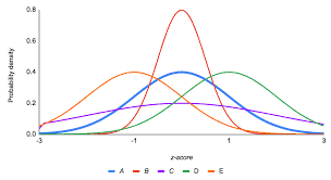
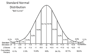
Most of the LaS distributions are of the continuous type. Examples are the general normal, Cauchy, and double-exponential (Laplace) distributions. If $\mu$ is the mean and $\sigma$ is the standard deviation of a univariate random variable $X$, and $Z=(X-\mu) / \sigma$ results in a standard distribution (devoid of parameters; see Section 1.1.2 in page 2), we say that $X$ belongs to the LaS family. This definition can easily be extended to the multivariate case where $\mu$ is a vector and $\Sigma$ is a matrix so that $Z=(X-\mu)^{\prime} \Sigma^{-1}(X-\mu)$ is in standard form. Sample data values are standardized using the transformation $z_{k}=\left(x_{k}-\bar{x}\right) / s_{x}$, where $s_{x}$ is the sample standard deviation, which can be applied to samples from any population including $\mathrm{LaS}$ distributions. The resulting values are called $z$-values or $z$-scores.
Write the above in univariate case as $X=\mu+\sigma Z$. As $\sigma$ is positive, a linear transformation with positive slope of any standard distribution results in a location-scale family for the underlying distribution. When $\sigma=1$, we get the one-parameter location family, and when $\mu=0$, we get the scale family. The exponential, gamma, Maxwell, Pareto, Rayleigh, Weibull, and halfnormal are scale-family distributions. The CDF of $X$ and $Z$ are related as $F((x-\mu) / \sigma)=G(x)$, and the quantile functions of $X$ and $Z$ are related as $F^{-1}(p)=\mu+\sigma G^{-1}(p)$. For $X$ continuous, the densities are related as $g(x)=(1 / \sigma) f((x-\mu) / \sigma)$. Maximum likelihood estimates (MLE) of the parameters of LaS distributions have some desirable properties. They are also easy to fit using available data. Extensions of this include $\log$-location-scale (LLS) distributions, nonlinearly transformed $\mathrm{LaS}$ distributions (like trigonometric, transcendental, and other functions of it, etc.) (Jones (2015) [80], Jones and Angela (2015) [81]).
工程统计代考
统计代写|工程统计代写engineering statistics代考|MOMENTS AND CUMULANTS
矩的概念在力学、粒子物理学、动力学气体理论等多个应用领域中都有使用。矩和累积量是统计分布的重要特征,对理解各自的分布起着重要作用。总体矩(也称为原始矩或零附近的矩)是随机变量幂的数学期望。它们用希腊字母表示为μr′=和(Xr), 对应的样本矩由米r′. 总概率的零时刻显然是一。第一个时刻是总体均值(即期望值X,μ=和(X))。对于非负连续分布,存在另一种期望公式和(X)=∫ll在l(1−F(X))dX, 在哪里ll是较低的和在l是上限。这采用简单且更熟悉的形式和(X)=∫0∞(1−F(X))dX=∫0∞小号(X)dX当范围是(0,∞). 当获得正矩时r是一个正整数,负时刻r是一个负整数,小数时刻r是一个实数。高阶矩也存在替代期望公式(参见[60]):
和(Xr)=∫0∞rXr−1(1−F(X))dX=∫0∞rXr−1小号(X)dX; 为了 r≥1.
中心矩是均值附近的矩,表示为μr=和((X−μ)r). 作为和(X)=μ,第一个中心矩总是为零,第二个中心矩是方差,第三个标准化矩是偏度,第四个标准化矩是峰度。
有几种可用的分散度量。示例是平均绝对偏差、方差(和标准偏差 (SD))、范围和变异系数 (CV)(SD 与平均值的比率(s/X¯n)对于一个样本,和σ/μ对于一个人口)。方差的一个特性是线性组合的方差独立于常数项(如果有)。数学上,曾是(C+bX)=|b|曾是(X)(没有常数 c)。类似地,如果变量是独立的,则线性组合的方差是方差的总和(曾是(X+是)=曾是(X)+曾是(是)). 这小号D是方差的正平方根,在金融和计量经济学中称为波动率。它用于数据标准化和一世=(X一世−X¯)/s在哪里s是个小号D一个样本(X1,X2,…,Xn). 可以组合归一化到相同比例或频率的数据。该技术用于光谱学、热力学、机器学习等多个应用领域。CV 量化了样本或总体内的相对变化。非常低的 CV 值表明组内的变化相对较小,而非常大的值不会提供太多有用的信息。它在生物信息学中用于过滤基因,这些基因通常以串行方式组合。它还在制造工程、教育和心理学中找到了应用,以比较异类群体之间的差异,因为它捕获了相对于平均值的变化水平。
反矩(也称为互反矩)是随机变量负幂的数学期望。逆矩存在的必要条件是F(0)=0, 对于χ2,F、beta、Weibull、Pareto、Rayleigh 和 Maxwell 分布。进一步来说,和(1/X)对于非负随机变量存在X当且当∫0d(F(X)/X)dX收敛一些小的d>0. 虽然阶乘矩可以用斯特林数来定义,但它们在连续分布中并不流行。具有负值和正值的随机变量的绝对矩定义为在ķ=和(|X|ķ)=∫−∞∞|X|ķF(X)dX=∫−∞∞|X|ķdF(X)
统计代写|工程统计代写engineering statistics代考|SIZE-BIASED DISTRIBUTIONS
任何具有有限平均值的统计分布都可以通过将 PDF 或 PMF 乘以C(1+ķX), 并选择C使得总概率变为一(ķ是用户选择的非零常数)。这减少到原始分布ķ=0(在这种情况下C=1)。未知C通过对离散的范围求和,对连续分布和混合分布进行积分来找到。这称为大小偏向分布 (SBD),它是加权分布的一种特殊情况。考虑 PDF 的连续均匀分布F(X;一个,b)=1/(b−一个)为了一个<X<b, 用 CUNI 表示(一个,b). 大小偏分布是G(是;一个,b,ķ)=[C/(b−一个)](1+ķ是). 这意味着任何离散的、连续的或混合的分布μ=和(X)存在可以提供大小有偏的分布。如章节所示2,CUNI(一个,b)有意思μ=(一个+b)/2. 综合以上从一个至b,并使用上面的结果得到[C/(b−一个)]∫一个b(1+ķ是)d是=1, 从中C=2/[2+ķ(一个+b)]=1/(1+ķμ). 类似地,指数 SBD 是G(是;ķ,λ)=Cλ(1+ķ是)经验(−λ是)在哪里C=λ2/(ķ+λ). 再举一个例子,著名的瑞利和麦克斯韦分布(在第二部分中讨论)实际上并不是新分布,而是简单的尺寸偏高斯分布ñ(0,一个2)带有偏置项X, 和ñ(0,ķ吨/米)带有偏置项X2, 分别。其他 SBD 将在各自的章节中讨论。
我们使用线性函数的期望(1+ķX)在上述公式中。这种技术可以扩展到作为权重的高阶多项式(例如,(1+bX+CX2)),以及一阶或更高阶的反矩,如果相应的矩存在的话。因此,如果和(1/(一个+ bX)) 存在于带有 PDF 的发行版中F(X), 我们可以形成一个新的 SBDG(X;一个,b,C)= CF(X)/(一个+bX)通过选择C从而使总概率统一。这个概念是由 Fisher (1934) [61] 引入的,用于模拟频率估计中的确定偏差,并由 Rao 扩展(1965,1984)[113,115]. 更一般地说,如果在(X)是具有有限期望的非负权函数(和(在(X))<∞), 然后在(X)F(X)/和(在(X))是加权分布的 PDF(在连续情况下;或 PMF 在离散情况下)。它有时被称为长度偏分布,当在(X)=X, 带 PDFG(X)=XF(X)/μ(因为重量X充当从某个固定参考点的长度)。作为一种特殊情况,我们可以使用和(Xķ)和和(X−ķ)当各自的秩序时刻ķ与 PDF 一起存在X±ķF(X)/μ±ķ′. 这导致属于同一家族的任一分布(如χ2, gamma, Pareto, Weibull, F, beta 和 power 定律),不同的已知族(大小偏置指数分布和(Xķ)导致伽马定律和幂律均匀分布),或全新的分布(学生 T、拉普拉斯、逆高斯等)。当普通矩不存在时,可以定义基于绝对矩的加权分布,如柯西分布(参见第 9.4 节,第 124 页)。分数幂也可用于获得正随机变量的新分布。其他函数,如对数(对于X≥0) 和指数可用于获得非线性加权分布。SBD 的概念适用于经典(离散和连续)分布以及截断、变换、取幂、偏斜、混合和其他扩展分布。
统计代写|工程统计代写engineering statistics代考|LOCATION-AND-SCALE DISTRIBUTIONS
LaS 分布是在一个参数中捕获位置信息(集中趋势)而在另一个参数中捕获尺度(分布和偏度)的分布。
定义 1.11 参数θ如果 PDF 的格式为,则称为位置参数F(X∓ θ), 如果 PDF 是以下形式,则为比例参数(1/θ)F(X/θ).
大多数 LaS 分布是连续类型的。示例是一般正态分布、柯西分布和双指数 (拉普拉斯) 分布。如果μ是平均值并且σ是单变量随机变量的标准差X, 和从=(X−μ)/σ导致标准分布(没有参数;参见第 2 页中的第 1.1.2 节),我们说X属于 LaS 家族。这个定义可以很容易地扩展到多元情况,其中μ是一个向量并且Σ是一个矩阵,所以从=(X−μ)′Σ−1(X−μ)是标准形式。使用转换对样本数据值进行标准化和ķ=(Xķ−X¯)/sX, 在哪里sX是样本标准差,它可以应用于来自任何总体的样本,包括大号一个小号分布。结果值被称为和-值或和-分数。
将上述单变量情况写为X=μ+σ从. 作为σ是正的,任何标准分布的正斜率的线性变换都会导致基础分布的位置尺度族。什么时候σ=1,我们得到单参数位置族,当μ=0,我们得到规模族。指数、伽马、麦克斯韦、帕累托、瑞利、威布尔和半正态分布是尺度系列分布。CDF 的X和从相关为F((X−μ)/σ)=G(X), 和分位数函数X和从相关为F−1(p)=μ+σG−1(p). 为了X连续,密度相关为G(X)=(1/σ)F((X−μ)/σ). LaS 分布参数的最大似然估计 (MLE) 具有一些理想的特性。它们也很容易使用可用数据进行拟合。对此的扩展包括日志-位置尺度(LLS)分布,非线性变换大号一个小号分布(如三角函数、超越函数和它的其他函数等)(Jones (2015) [80]、Jones and Angela (2015) [81])。

统计代写请认准statistics-lab™. statistics-lab™为您的留学生涯保驾护航。
金融工程代写
金融工程是使用数学技术来解决金融问题。金融工程使用计算机科学、统计学、经济学和应用数学领域的工具和知识来解决当前的金融问题,以及设计新的和创新的金融产品。
非参数统计代写
非参数统计指的是一种统计方法,其中不假设数据来自于由少数参数决定的规定模型;这种模型的例子包括正态分布模型和线性回归模型。
广义线性模型代考
广义线性模型(GLM)归属统计学领域,是一种应用灵活的线性回归模型。该模型允许因变量的偏差分布有除了正态分布之外的其它分布。
术语 广义线性模型(GLM)通常是指给定连续和/或分类预测因素的连续响应变量的常规线性回归模型。它包括多元线性回归,以及方差分析和方差分析(仅含固定效应)。
有限元方法代写
有限元方法(FEM)是一种流行的方法,用于数值解决工程和数学建模中出现的微分方程。典型的问题领域包括结构分析、传热、流体流动、质量运输和电磁势等传统领域。
有限元是一种通用的数值方法,用于解决两个或三个空间变量的偏微分方程(即一些边界值问题)。为了解决一个问题,有限元将一个大系统细分为更小、更简单的部分,称为有限元。这是通过在空间维度上的特定空间离散化来实现的,它是通过构建对象的网格来实现的:用于求解的数值域,它有有限数量的点。边界值问题的有限元方法表述最终导致一个代数方程组。该方法在域上对未知函数进行逼近。[1] 然后将模拟这些有限元的简单方程组合成一个更大的方程系统,以模拟整个问题。然后,有限元通过变化微积分使相关的误差函数最小化来逼近一个解决方案。
tatistics-lab作为专业的留学生服务机构,多年来已为美国、英国、加拿大、澳洲等留学热门地的学生提供专业的学术服务,包括但不限于Essay代写,Assignment代写,Dissertation代写,Report代写,小组作业代写,Proposal代写,Paper代写,Presentation代写,计算机作业代写,论文修改和润色,网课代做,exam代考等等。写作范围涵盖高中,本科,研究生等海外留学全阶段,辐射金融,经济学,会计学,审计学,管理学等全球99%专业科目。写作团队既有专业英语母语作者,也有海外名校硕博留学生,每位写作老师都拥有过硬的语言能力,专业的学科背景和学术写作经验。我们承诺100%原创,100%专业,100%准时,100%满意。
随机分析代写
随机微积分是数学的一个分支,对随机过程进行操作。它允许为随机过程的积分定义一个关于随机过程的一致的积分理论。这个领域是由日本数学家伊藤清在第二次世界大战期间创建并开始的。
时间序列分析代写
随机过程,是依赖于参数的一组随机变量的全体,参数通常是时间。 随机变量是随机现象的数量表现,其时间序列是一组按照时间发生先后顺序进行排列的数据点序列。通常一组时间序列的时间间隔为一恒定值(如1秒,5分钟,12小时,7天,1年),因此时间序列可以作为离散时间数据进行分析处理。研究时间序列数据的意义在于现实中,往往需要研究某个事物其随时间发展变化的规律。这就需要通过研究该事物过去发展的历史记录,以得到其自身发展的规律。
回归分析代写
多元回归分析渐进(Multiple Regression Analysis Asymptotics)属于计量经济学领域,主要是一种数学上的统计分析方法,可以分析复杂情况下各影响因素的数学关系,在自然科学、社会和经济学等多个领域内应用广泛。
MATLAB代写
MATLAB 是一种用于技术计算的高性能语言。它将计算、可视化和编程集成在一个易于使用的环境中,其中问题和解决方案以熟悉的数学符号表示。典型用途包括:数学和计算算法开发建模、仿真和原型制作数据分析、探索和可视化科学和工程图形应用程序开发,包括图形用户界面构建MATLAB 是一个交互式系统,其基本数据元素是一个不需要维度的数组。这使您可以解决许多技术计算问题,尤其是那些具有矩阵和向量公式的问题,而只需用 C 或 Fortran 等标量非交互式语言编写程序所需的时间的一小部分。MATLAB 名称代表矩阵实验室。MATLAB 最初的编写目的是提供对由 LINPACK 和 EISPACK 项目开发的矩阵软件的轻松访问,这两个项目共同代表了矩阵计算软件的最新技术。MATLAB 经过多年的发展,得到了许多用户的投入。在大学环境中,它是数学、工程和科学入门和高级课程的标准教学工具。在工业领域,MATLAB 是高效研究、开发和分析的首选工具。MATLAB 具有一系列称为工具箱的特定于应用程序的解决方案。对于大多数 MATLAB 用户来说非常重要,工具箱允许您学习和应用专业技术。工具箱是 MATLAB 函数(M 文件)的综合集合,可扩展 MATLAB 环境以解决特定类别的问题。可用工具箱的领域包括信号处理、控制系统、神经网络、模糊逻辑、小波、仿真等。