如果你也在 怎样代写应用时间序列分析applied time series analysis这个学科遇到相关的难题,请随时右上角联系我们的24/7代写客服。
时间序列分析applied time series analysis是分析在一个时间间隔内收集的一系列数据点的具体方式。在时间序列分析applied time series analysis中,分析人员在设定的时间段内以一致的时间间隔记录数据点,而不仅仅是间歇性或随机地记录数据点。
statistics-lab™ 为您的留学生涯保驾护航 在代写应用时间序列分析applied time series analysis方面已经树立了自己的口碑, 保证靠谱, 高质且原创的统计Statistics代写服务。我们的专家在代写应用时间序列分析applied time series analysis方面经验极为丰富,各种代写应用时间序列分析applied time series analysis相关的作业也就用不着说。
我们提供的应用时间序列分析applied time series analysis及其相关学科的代写,服务范围广, 其中包括但不限于:
- Statistical Inference 统计推断
- Statistical Computing 统计计算
- Advanced Probability Theory 高等楖率论
- Advanced Mathematical Statistics 高等数理统计学
- (Generalized) Linear Models 广义线性模型
- Statistical Machine Learning 统计机器学习
- Longitudinal Data Analysis 纵向数据分析
- Foundations of Data Science 数据科学基础
统计代写|应用时间序列分析代写applied time series anakysis代考|SIMPLE AUTOREGRESSIVE MODELS
The fact that the monthly return $r_{I}$ of CRSP value-weighted index has a statistically significant lag-l autocorrelation indicates that the lagged return $r_{t-1}$ might be useful in predicting $r_{t}$. A simple model that makes use of such predictive power is
$$
r_{t}=\phi_{0}+\phi_{1} r_{t-1}+a_{l}
$$
where $\left{a_{t}\right}$ is assumed to be a white noise series with mean zero and variance $\sigma_{a}^{2}$. This model is in the same form as the well-known simple linear regression model in
which $r_{I}$ is the dependent variable and $r_{t-1}$ is the explanatory variable. In the time series literature, Model (2.6) is referred to as a simple autoregressive (AR) model of order 1 or simply an AR(1) model. This simple model is also widely used in stochastic volatility modeling when $r_{t}$ is replaced by its log volatility; see Chapters 3 and $10 .$
The AR(1) model in Eq. (2.6) has several properties similar to those of the simple linear regression model. However, there are some significant differences between the two models, which we discuss later. Here it suffices to note that an $\mathrm{AR}(1)$ model implies that, conditional on the past return $r_{t-1}$, we have
$$
E\left(r_{t} \mid r_{t-1}\right)=\phi_{0}+\phi_{1} r_{t-1}, \quad \operatorname{Var}\left(r_{t} \mid r_{t-1}\right)=\operatorname{Var}\left(a_{t}\right)=\sigma_{a}^{2}
$$
That is, given the past return $r_{t-1}$, the current return is centered around $\phi_{0}+\phi_{1} r_{t-1}$ with variability $\sigma_{a}^{2}$. This is a Markov property such that conditional on $r_{t-1}$, the return $r_{t}$ is not correlated with $r_{t-i}$ for $i>1$. Obviously, there are situations in which $r_{t-1}$ alone cannot determine the conditional expectation of $r_{t}$ and a more flexible model must be sought. A straightforward generalization of the AR(1) model is the $\mathrm{AR}(p)$ model
$$
r_{t}=\phi_{0}+\phi_{1} r_{t-1}+\cdots+\phi_{p} r_{t-p}+a_{t}
$$
where $p$ is a non-negative integer and $\left{a_{t}\right}$ is defined in Eq. (2.6). This model says that the past $p$ values $r_{l-i}(i=1, \ldots, p)$ jointly determine the conditional expectation of $r_{t}$ given the past data. The $\operatorname{AR}(p)$ model is in the same form as a multiple linear regression model with lagged values serving as the explanatory variables.
统计代写|应用时间序列分析代写applied time series anakysis代考| AR(1) Model
We begin with the sufficient and necessary condition for weak stationarity of the AR(1) model in Eq. (2.6). Assuming that the series is weakly stationary, we have $E\left(r_{t}\right)=\mu, \operatorname{Var}\left(r_{t}\right)=\gamma_{0}$, and $\operatorname{Cov}\left(r_{t}, r_{t-j}\right)=\gamma_{j}$, where $\mu$ and $\gamma_{0}$ are constant and $\gamma_{j}$ is a function of $j$, not $t$. We can easily obtain the mean, variance, and autocorrelations of the series as follows. Taking the expectation of Eq. (2.6) and because $E\left(a_{t}\right)=0$, we obtain
$$
E\left(r_{t}\right)=\phi_{0}+\phi_{1} E\left(r_{I-1}\right)
$$
Under the stationarity condition, $E\left(r_{t}\right)=E\left(r_{I-1}\right)=\mu$ and hence
$$
\mu=\phi_{0}+\phi_{1} \mu \quad \text { or } \quad E\left(r_{t}\right)=\mu=\frac{\phi_{0}}{1-\phi_{1}}
$$
This result has two implications for $r_{t}$. First, the mean of $r_{I}$ exists if $\phi_{1} \neq 1$. Second, the mean of $r_{t}$ is zero if and only if $\phi_{0}=0$. Thus, for a stationary AR(1) process, the constant term $\phi_{0}$ is related to the mean of $r_{t}$ and $\phi_{0}=0$ implies that $E\left(r_{t}\right)=0$.
Next, using $\phi_{0}=\left(1-\phi_{1}\right) \mu$, the AR(1) model can be rewritten as
$$
r_{t}-\mu=\phi_{1}\left(r_{t-1}-\mu\right)+a_{t}
$$
By repeated substitutions, the prior equation implies that
$$
\begin{aligned}
r_{t}-\mu &=a_{t}+\phi_{1} a_{t-1}+\phi_{1}^{2} a_{t-2}+\cdots \
&=\sum_{i=0}^{\infty} \phi_{1}^{i} a_{t-i}
\end{aligned}
$$
Thus, $r_{t}-\mu$ is a linear function of $a_{t-i}$ for $i \geq 0$. Using this property and the independence of the series $\left{a_{t}\right}$, we obtain $E\left[\left(r_{t}-\mu\right) a_{t+1}\right]=0$. By the stationarity assumption, we have $\operatorname{Cov}\left(r_{t-1}, a_{t}\right)=E\left[\left(r_{t-1}-\mu\right) a_{t}\right]=0$. This latter result can also be seen from the fact that $r_{t-1}$ occurred before time $t$ and $a_{t}$ does not depend on any past information. Taking the square, then the expectation of Eq. (2.8), we obtain
$$
\operatorname{Var}\left(r_{t}\right)=\phi_{1}^{2} \operatorname{Var}\left(r_{t-1}\right)+\sigma_{a}^{2},
$$
where $\sigma_{a}^{2}$ is the variance of $a_{l}$ and we make use of the fact that the covariance between $r_{t-1}$ and $a_{t}$ is zero. Under the stationarity assumption, $\operatorname{Var}\left(r_{t}\right)=\operatorname{Var}\left(r_{t-1}\right)$, so that
$$
\operatorname{Var}\left(r_{I}\right)=\frac{\sigma_{a}^{2}}{1-\phi_{1}^{2}}
$$
provided that $\phi_{1}^{2}<1$. The requirement of $\phi_{1}^{2}<1$ results from the fact that the variance of a random variable is bounded and non-negative. Consequently, the weak stationarity of an AR(1) model implies that $-1<\phi_{1}<1$. Yet if $-1<\phi_{1}<1$, then by Eq. $(2.9)$ and the independence of the $\left{a_{t}\right}$ series, we can show that the mean and variance of $r_{t}$ are finite. In addition, by the Cauchy-Schwartz inequality, all the autocovariances of $r_{t}$ are finite. Therefore, the $\mathrm{AR}(1)$ model is weakly stationary. In summary, the necessary and sufficient condition for the AR(1) model in Eq. (2.6) to be weakly stationary is $\left|\phi_{1}\right|<1$.
统计代写|应用时间序列分析代写applied time series anakysis代考|Autocorrelation Function of an AR(1) Model
Multiplying Eq. (2.8) by $a_{t}$, using the independence between $a_{t}$ and $r_{t-1}$, and taking expectation, we obtain
$$
E\left[a_{t}\left(r_{t}-\mu\right)\right]=E\left[a_{t}\left(r_{t-1}-\mu\right)\right]+E\left(a_{t}^{2}\right)=E\left(a_{t}^{2}\right)=\sigma_{a}^{2}
$$
where $\sigma_{a}^{2}$ is the variance of $a_{t}$. Multiplying Eq. $(2.8)$ by $\left(r_{t-\ell}-\mu\right)$, taking expectation, and using the prior result, we have
$$
\gamma_{\ell}= \begin{cases}\phi_{1} \gamma_{1}+\sigma_{a}^{2} & \text { if } \ell=0 \ \phi_{1} \gamma_{\ell-1} & \text { if } \ell>0\end{cases}
$$
where we use $\gamma_{\ell}=\gamma_{-\ell}$. Consequently, for a weakly stationary AR(1) model in Eq. (2.6), we have
$$
\operatorname{Var}\left(r_{t}\right)=\gamma_{0}=\frac{\sigma^{2}}{1-\phi_{1}^{2}}, \quad \text { and } \quad \gamma_{\ell}=\phi_{1} \gamma_{\ell-1}, \quad \text { for } \quad \ell>0
$$
From the latter equation, the ACF of $r_{t}$ satisfies
$$
\rho_{\ell}=\phi_{1} \rho_{\ell-1}, \quad \text { for } \quad \ell \geq 0
$$
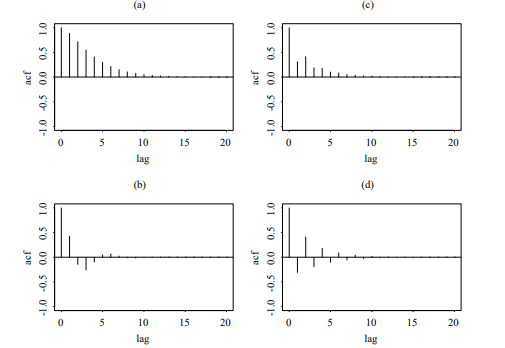
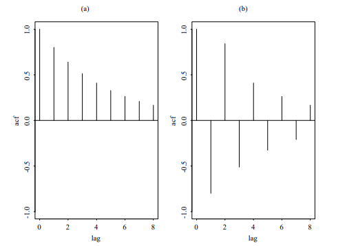
Because $\rho_{0}=1$, we have $\rho_{\ell}=\phi_{1}^{\ell}$. This result says that the ACF of a weakly stationary AR(1) series decays exponentially with rate $\phi_{1}$ and starting value $\rho_{0}=1$. For a positive $\phi_{1}$, the plot of ACF of an AR(1) model shows a nice exponential decay.
时间序列分析代写
统计代写|应用时间序列分析代写applied time series anakysis代考|SIMPLE AUTOREGRESSIVE MODELS
每月回报的事实r一世的 CRSP 价值加权指数具有统计显着的滞后 l 自相关表明滞后回报r吨−1可能对预测有用r吨. 一个利用这种预测能力的简单模型是
r吨=φ0+φ1r吨−1+一种l
在哪里\left{a_{t}\right}\left{a_{t}\right}假设是一个均值为零和方差的白噪声序列σ一种2. 该模型与著名的简单线性回归模型的形式相同
哪一个r一世是因变量,并且r吨−1是解释变量。在时间序列文献中,模型 (2.6) 被称为简单的 1 阶自回归 (AR) 模型或简称为 AR(1) 模型。这种简单的模型也广泛用于随机波动率建模,当r吨被它的对数波动率取代;见第 3 章和10.
方程式中的 AR(1)模型。(2.6) 有几个与简单线性回归模型相似的性质。但是,这两种模型之间存在一些显着差异,我们将在后面讨论。这里只需要注意一个一种R(1)模型意味着,以过去的回报为条件r吨−1, 我们有
和(r吨∣r吨−1)=φ0+φ1r吨−1,曾是(r吨∣r吨−1)=曾是(一种吨)=σ一种2
也就是说,给定过去的回报r吨−1,当前回报集中在φ0+φ1r吨−1具有可变性σ一种2. 这是一个马尔可夫性质,使得条件r吨−1, 回报r吨不相关r吨−一世为了一世>1. 显然,在某些情况下r吨−1单独无法确定条件期望r吨并且必须寻求更灵活的模式。AR(1) 模型的简单概括是一种R(p)模型
r吨=φ0+φ1r吨−1+⋯+φpr吨−p+一种吨
在哪里p是一个非负整数并且\left{a_{t}\right}\left{a_{t}\right}在方程式中定义。(2.6)。这个模型说过去p价值观rl−一世(一世=1,…,p)共同确定条件期望r吨给定过去的数据。这和(p)模型与以滞后值作为解释变量的多元线性回归模型的形式相同。
统计代写|应用时间序列分析代写applied time series anakysis代考| AR(1) Model
我们从方程中 AR(1) 模型的弱平稳性的充分必要条件开始。(2.6)。假设序列是弱平稳的,我们有和(r吨)=μ,曾是(r吨)=C0, 和这(r吨,r吨−j)=Cj, 在哪里μ和C0是恒定的并且Cj是一个函数j, 不是吨. 我们可以很容易地得到序列的均值、方差和自相关,如下所示。以方程的期望。(2.6) 并且因为和(一种吨)=0, 我们获得
和(r吨)=φ0+φ1和(r一世−1)
在平稳条件下,和(r吨)=和(r一世−1)=μ因此
μ=φ0+φ1μ 或者 和(r吨)=μ=φ01−φ1
这个结果有两个含义r吨. 首先,平均值r一世如果存在φ1≠1. 二、均值r吨为零当且仅当φ0=0. 因此,对于一个平稳的 AR(1) 过程,常数项φ0与平均值有关r吨和φ0=0暗示和(r吨)=0.
接下来,使用φ0=(1−φ1)μ, AR(1) 模型可以改写为
r吨−μ=φ1(r吨−1−μ)+一种吨
通过重复替换,先验方程意味着
r吨−μ=一种吨+φ1一种吨−1+φ12一种吨−2+⋯ =∑一世=0∞φ1一世一种吨−一世
因此,r吨−μ是一个线性函数一种吨−一世为了一世≥0. 使用这个属性和级数的独立性\left{a_{t}\right}\left{a_{t}\right}, 我们获得和[(r吨−μ)一种吨+1]=0. 根据平稳性假设,我们有这(r吨−1,一种吨)=和[(r吨−1−μ)一种吨]=0. 后一种结果也可以从以下事实中看出r吨−1发生在时间之前吨和一种吨不依赖于任何过去的信息。取平方,然后是等式的期望。(2.8),我们得到
曾是(r吨)=φ12曾是(r吨−1)+σ一种2,
在哪里σ一种2是方差一种l我们利用了以下事实:r吨−1和一种吨为零。在平稳性假设下,曾是(r吨)=曾是(r吨−1), 以便
曾是(r一世)=σ一种21−φ12
前提是φ12<1. 的要求φ12<1这是由于随机变量的方差是有界的且非负的。因此,AR(1) 模型的弱平稳性意味着−1<φ1<1. 然而如果−1<φ1<1,然后由等式。(2.9)和独立性\left{a_{t}\right}\left{a_{t}\right}系列,我们可以证明,均值和方差r吨是有限的。此外,通过 Cauchy-Schwartz 不等式,所有的自协方差r吨是有限的。因此,一种R(1)模型是弱平稳的。总之,等式中AR(1)模型的充要条件。(2.6) 弱静止是|φ1|<1.
统计代写|应用时间序列分析代写applied time series anakysis代考|Autocorrelation Function of an AR(1) Model
乘法方程。(2.8) 由一种吨, 使用之间的独立性一种吨和r吨−1,并取期望,我们得到
和[一种吨(r吨−μ)]=和[一种吨(r吨−1−μ)]+和(一种吨2)=和(一种吨2)=σ一种2
在哪里σ一种2是方差一种吨. 乘法方程。(2.8)经过(r吨−ℓ−μ),取期望,并使用先前的结果,我们有
Cℓ={φ1C1+σ一种2 如果 ℓ=0 φ1Cℓ−1 如果 ℓ>0
我们在哪里使用Cℓ=C−ℓ. 因此,对于方程中的弱平稳 AR(1) 模型。(2.6),我们有
曾是(r吨)=C0=σ21−φ12, 和 Cℓ=φ1Cℓ−1, 为了 ℓ>0
从后一个方程,ACFr吨满足
ρℓ=φ1ρℓ−1, 为了 ℓ≥0
因为ρ0=1, 我们有ρℓ=φ1ℓ. 这个结果表明弱平稳 AR(1) 系列的 ACF 随速率呈指数衰减φ1和起始值ρ0=1. 对于一个积极的φ1,AR(1) 模型的 ACF 图显示出很好的指数衰减。

统计代写请认准statistics-lab™. statistics-lab™为您的留学生涯保驾护航。统计代写|python代写代考
随机过程代考
在概率论概念中,随机过程是随机变量的集合。 若一随机系统的样本点是随机函数,则称此函数为样本函数,这一随机系统全部样本函数的集合是一个随机过程。 实际应用中,样本函数的一般定义在时间域或者空间域。 随机过程的实例如股票和汇率的波动、语音信号、视频信号、体温的变化,随机运动如布朗运动、随机徘徊等等。
贝叶斯方法代考
贝叶斯统计概念及数据分析表示使用概率陈述回答有关未知参数的研究问题以及统计范式。后验分布包括关于参数的先验分布,和基于观测数据提供关于参数的信息似然模型。根据选择的先验分布和似然模型,后验分布可以解析或近似,例如,马尔科夫链蒙特卡罗 (MCMC) 方法之一。贝叶斯统计概念及数据分析使用后验分布来形成模型参数的各种摘要,包括点估计,如后验平均值、中位数、百分位数和称为可信区间的区间估计。此外,所有关于模型参数的统计检验都可以表示为基于估计后验分布的概率报表。
广义线性模型代考
广义线性模型(GLM)归属统计学领域,是一种应用灵活的线性回归模型。该模型允许因变量的偏差分布有除了正态分布之外的其它分布。
statistics-lab作为专业的留学生服务机构,多年来已为美国、英国、加拿大、澳洲等留学热门地的学生提供专业的学术服务,包括但不限于Essay代写,Assignment代写,Dissertation代写,Report代写,小组作业代写,Proposal代写,Paper代写,Presentation代写,计算机作业代写,论文修改和润色,网课代做,exam代考等等。写作范围涵盖高中,本科,研究生等海外留学全阶段,辐射金融,经济学,会计学,审计学,管理学等全球99%专业科目。写作团队既有专业英语母语作者,也有海外名校硕博留学生,每位写作老师都拥有过硬的语言能力,专业的学科背景和学术写作经验。我们承诺100%原创,100%专业,100%准时,100%满意。
机器学习代写
随着AI的大潮到来,Machine Learning逐渐成为一个新的学习热点。同时与传统CS相比,Machine Learning在其他领域也有着广泛的应用,因此这门学科成为不仅折磨CS专业同学的“小恶魔”,也是折磨生物、化学、统计等其他学科留学生的“大魔王”。学习Machine learning的一大绊脚石在于使用语言众多,跨学科范围广,所以学习起来尤其困难。但是不管你在学习Machine Learning时遇到任何难题,StudyGate专业导师团队都能为你轻松解决。
多元统计分析代考
基础数据: $N$ 个样本, $P$ 个变量数的单样本,组成的横列的数据表
变量定性: 分类和顺序;变量定量:数值
数学公式的角度分为: 因变量与自变量
时间序列分析代写
随机过程,是依赖于参数的一组随机变量的全体,参数通常是时间。 随机变量是随机现象的数量表现,其时间序列是一组按照时间发生先后顺序进行排列的数据点序列。通常一组时间序列的时间间隔为一恒定值(如1秒,5分钟,12小时,7天,1年),因此时间序列可以作为离散时间数据进行分析处理。研究时间序列数据的意义在于现实中,往往需要研究某个事物其随时间发展变化的规律。这就需要通过研究该事物过去发展的历史记录,以得到其自身发展的规律。
回归分析代写
多元回归分析渐进(Multiple Regression Analysis Asymptotics)属于计量经济学领域,主要是一种数学上的统计分析方法,可以分析复杂情况下各影响因素的数学关系,在自然科学、社会和经济学等多个领域内应用广泛。
MATLAB代写
MATLAB 是一种用于技术计算的高性能语言。它将计算、可视化和编程集成在一个易于使用的环境中,其中问题和解决方案以熟悉的数学符号表示。典型用途包括:数学和计算算法开发建模、仿真和原型制作数据分析、探索和可视化科学和工程图形应用程序开发,包括图形用户界面构建MATLAB 是一个交互式系统,其基本数据元素是一个不需要维度的数组。这使您可以解决许多技术计算问题,尤其是那些具有矩阵和向量公式的问题,而只需用 C 或 Fortran 等标量非交互式语言编写程序所需的时间的一小部分。MATLAB 名称代表矩阵实验室。MATLAB 最初的编写目的是提供对由 LINPACK 和 EISPACK 项目开发的矩阵软件的轻松访问,这两个项目共同代表了矩阵计算软件的最新技术。MATLAB 经过多年的发展,得到了许多用户的投入。在大学环境中,它是数学、工程和科学入门和高级课程的标准教学工具。在工业领域,MATLAB 是高效研究、开发和分析的首选工具。MATLAB 具有一系列称为工具箱的特定于应用程序的解决方案。对于大多数 MATLAB 用户来说非常重要,工具箱允许您学习和应用专业技术。工具箱是 MATLAB 函数(M 文件)的综合集合,可扩展 MATLAB 环境以解决特定类别的问题。可用工具箱的领域包括信号处理、控制系统、神经网络、模糊逻辑、小波、仿真等。