如果你也在 怎样代写应用时间序列分析applied time series analysis这个学科遇到相关的难题,请随时右上角联系我们的24/7代写客服。
时间序列分析applied time series analysis是分析在一个时间间隔内收集的一系列数据点的具体方式。在时间序列分析applied time series analysis中,分析人员在设定的时间段内以一致的时间间隔记录数据点,而不仅仅是间歇性或随机地记录数据点。
statistics-lab™ 为您的留学生涯保驾护航 在代写应用时间序列分析applied time series analysis方面已经树立了自己的口碑, 保证靠谱, 高质且原创的统计Statistics代写服务。我们的专家在代写应用时间序列分析applied time series analysis方面经验极为丰富,各种代写应用时间序列分析applied time series analysis相关的作业也就用不着说。
我们提供的应用时间序列分析applied time series analysis及其相关学科的代写,服务范围广, 其中包括但不限于:
- Statistical Inference 统计推断
- Statistical Computing 统计计算
- Advanced Probability Theory 高等楖率论
- Advanced Mathematical Statistics 高等数理统计学
- (Generalized) Linear Models 广义线性模型
- Statistical Machine Learning 统计机器学习
- Longitudinal Data Analysis 纵向数据分析
- Foundations of Data Science 数据科学基础
统计代写|应用时间序列分析代写applied time series anakysis代考|Portmanteau Test
Financial applications often require to test jointly that several autocorrelations of $r_{I}$ are zero. Box and Pierce (1970) propose the Portmanteau statistic
$$
Q^{}(m)=T \sum_{\ell=1}^{m} \hat{\rho}{\ell}^{2} $$ as a test statistic for the null hypothesis $H{o}: \rho_{1}=\cdots=\rho_{m}=0$ against the alternative hypothesis $H_{a}: \rho_{i} \neq 0$ for some $i \in{1, \ldots, m}$. Under the assumption that $\left{r_{t}\right}$ is an iid sequence with certain moment conditions, $Q^{}(\mathrm{~m})$ is asymptotically a chi-squared random variable with $m$ degrees of freedom.
Ljung and Box (1978) modify the $Q^{*}(\mathrm{~m})$ statistic as below to increase the power of the test in finite samples,
$$
Q(m)=T(T+2) \sum_{\ell=1}^{m} \frac{\hat{\rho}_{\ell}^{2}}{T-\ell} .
$$
In practice, the selection of $m$ may affect the performance of the $Q(m)$ statistic. Several values of $m$ are often used. Simulation studies suggest that the choice of $m \approx \ln (T)$ provides better power performance.
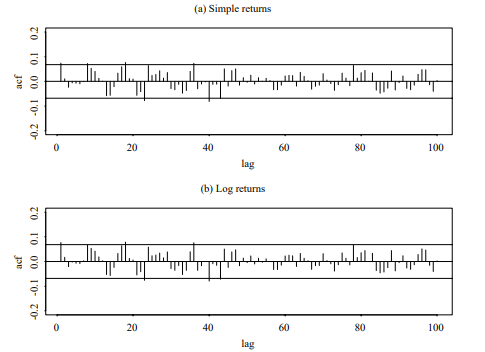
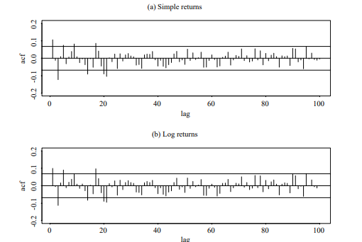
The function $\hat{\rho}{1}, \hat{\rho}{2}, \ldots$ is called the sample autocorrelation function (ACF) of $r_{t}$. It plays an important role in linear time series analysis. As a matter of fact, a linear time series model can be characterized by its ACF, and linear time series modeling makes use of the sample ACF to capture the linear dynamic of the data. Figure $2.1$ shows the sample autocorrelation functions of monthly simple and log returns of IBM stock from January 1926 to December 1997. The two sample ACFs are very close to each other, and they suggest that the serial correlations of monthly IBM stock returns are very small, if any. The sample ACFs are all within their two standard-error limits, indicating that they are not significant at the $5 \%$ level. In addition, for the simple returns, the Ljung-Box statistics give $Q(5)=5.4$ and $Q(10)=14.1$, which correspond to $p$ value of $0.37$ and $0.17$, respectively, based on chi-squared distributions with 5 and 10 degrees of freedom. For the log returns, we have $Q(5)=5.8$ and $Q(10)=13.7$ with $p$ value $0.33$ and $0.19$, respectively. The joint tests confirm that monthly IBM stock returns have no significant serial correlations. Figure $2.2$ shows the same for the monthly returns of the value-weighted index from the Center for Research in Security Prices (CRSP), University of Chicago. There are some significant serial correlations at the $5 \%$ level for both return series. The Ljung-Box statistics give $Q(5)=27.8$ and $Q(10)=36.0$ for the simple returns and $Q(5)=26.9$
统计代写|应用时间序列分析代写applied time series anakysis代考| WHITE NOISE AND LINEAR TIME SERIES
A time series $r_{t}$ is called a white noise if $\left{r_{t}\right}$ is a sequence of independent and identically distributed random variables with finite mean and variance. In particular,
Figure 2.2. Sample autocorrelation functions of monthly simple and log returns of the valueweighted index of U.S. Markets from January 1926 to December 1997. In each plot, the two horizontal lines denote two standard-error limits of the sample ACF.
if $r_{t}$ is normally distributed with mean zero and variance $\sigma^{2}$, the series is called a Gaussian white noise. For a white noise series, all the ACFs are zero. In practice, if all sample ACFs are close to zero, then the series is a white noise series. Based on Figures $2.1$ and $2.2$, the monthly returns of IBM stock are close to white noise, whereas those of the value-weighted index are not.
The behavior of sample autocorrelations of the value-weighted index returns indicates that for some asset returns it is necessary to model the serial dependence before further analysis can be made. In what follows, we discuss some simple time series models that are useful in modeling the dynamic structure of a time series. The concepts presented are also useful later in modeling volatility of asset returns.
统计代写|应用时间序列分析代写applied time series anakysis代考|Linear Time Series
A time series $r_{I}$ is said to be linear if it can be written as
$$
r_{t}=\mu+\sum_{i=0}^{\infty} \psi_{i} a_{t-i}
$$
where $\mu$ is the mean of $r_{t}, \psi_{0}=1$ and $\left{a_{t}\right}$ is a sequence of independent and identically distributed random variables with mean zero and a well-defined distribution (i.e., $\left{a_{t}\right}$ is a white noise series). In this book, we are mainly concerned with the case where $a_{t}$ is a continuous random variable. Not all financial time series are linear, however. We study nonlinearity and nonlinear models in Chapter $4 .$
For a linear time series in Eq. (2.4), the dynamic structure of $r_{l}$ is governed by the coefficients $\psi_{i}$, which are called the $\psi$-weights of $r_{t}$ in the time series literature. If $r_{t}$ is weakly stationary, we can obtain its mean and variance easily by using the independence of $\left{a_{t}\right}$ as
$$
E\left(r_{t}\right)=\mu, \quad \operatorname{Var}\left(r_{t}\right)=\sigma_{a}^{2} \sum_{i=0}^{\infty} \psi_{i}^{2},
$$
where $\sigma_{a}^{2}$ is the variance of $a_{t}$. Furthermore, the lag- $\ell$ autocovariance of $r_{t}$ is
$$
\begin{aligned}
\gamma_{\ell} &=\operatorname{Cov}\left(r_{t}, r_{t-\ell}\right)=E\left[\left(\sum_{i=0}^{\infty} \psi_{i} a_{t-i}\right)\left(\sum_{j=0}^{\infty} \psi_{j} a_{t-\ell-j}\right)\right] \
&=E\left(\sum_{i, j=0}^{\infty} \psi_{i} \psi_{j} a_{t-i} a_{t-\ell-j}\right) \
&=\sum_{j=0}^{\infty} \psi_{j+\ell} \psi_{j} E\left(a_{t-\ell-j}^{2}\right)=\sigma_{a}^{2} \sum_{j=0}^{\infty} \psi_{j} \psi_{j+\ell}
\end{aligned}
$$
Consequently, the $\psi$-weights are related to the autocorrelations of $r_{t}$ as follows:
$$
\rho_{\ell}=\frac{\gamma_{\ell}}{\gamma_{0}}=\frac{\sum_{i=0}^{\infty} \psi_{i} \psi_{i+\ell}}{1+\sum_{i=1}^{\infty} \psi_{i}^{2}}, \quad \ell \geq 0,
$$
where $\psi_{0}=1$. Linear time series models are econometric and statistical models used to describe the pattern of the $\psi$-weights of $r_{t}$.
时间序列分析代写
统计代写|应用时间序列分析代写applied time series anakysis代考|Portmanteau Test
金融应用程序通常需要联合测试几个自相关r一世为零。Box 和 Pierce (1970) 提出了 Portmanteau 统计量
问(米)=吨∑ℓ=1米ρ^ℓ2作为零假设的检验统计量H这:ρ1=⋯=ρ米=0反对备择假设H一种:ρ一世≠0对于一些一世∈1,…,米. 在假设下\左{r_{t}\右}\左{r_{t}\右}是具有特定矩条件的独立同分布序列,问( 米)是渐近的卡方随机变量米自由程度。
Ljung 和 Box (1978) 修改了问∗( 米)统计如下,以增加有限样本中的检验能力,
问(米)=吨(吨+2)∑ℓ=1米ρ^ℓ2吨−ℓ.
在实践中,选择米可能会影响性能问(米)统计。的几个值米经常使用。模拟研究表明,选择米≈ln(吨)提供更好的电源性能。
功能ρ^1,ρ^2,…称为样本自相关函数(ACF)r吨. 它在线性时间序列分析中起着重要作用。事实上,线性时间序列模型可以通过其 ACF 来表征,线性时间序列建模利用样本 ACF 来捕捉数据的线性动态。数字2.1显示了 1926 年 1 月至 1997 年 12 月 IBM 股票月度简单收益和对数收益的样本自相关函数。两个样本 ACF 非常接近,它们表明 IBM 股票月收益的序列相关性非常小,如果有的话. 样本 ACF 都在它们的两个标准误差范围内,表明它们在5%等级。此外,对于简单收益,Ljung-Box 统计量给出问(5)=5.4和问(10)=14.1, 对应于p的价值0.37和0.17,分别基于具有 5 和 10 自由度的卡方分布。对于日志返回,我们有问(5)=5.8和问(10)=13.7和p价值0.33和0.19, 分别。联合测试证实,每月 IBM 股票收益没有显着的序列相关性。数字2.2芝加哥大学证券价格研究中心 (CRSP) 的价值加权指数的月回报率显示相同。存在一些显着的序列相关性5%两个返回系列的水平。Ljung-Box 统计数据给出问(5)=27.8和问(10)=36.0对于简单的回报和问(5)=26.9
统计代写|应用时间序列分析代写applied time series anakysis代考| WHITE NOISE AND LINEAR TIME SERIES
一个时间序列r吨称为白噪声,如果\左{r_{t}\右}\左{r_{t}\右}是一系列具有有限均值和方差的独立同分布随机变量。尤其,
图 2.2。1926 年 1 月至 1997 年 12 月美国市场价值加权指数的每月简单和对数回报的样本自相关函数。在每个图中,两条水平线表示样本 ACF 的两个标准误差限制。
如果r吨正态分布,均值为 0,方差为σ2,该系列称为高斯白噪声。对于白噪声系列,所有 ACF 都为零。在实践中,如果所有样本 ACF 都接近于零,则该系列是白噪声系列。基于数字2.1和2.2,IBM 股票的月收益接近于白噪声,而价值加权指数则不然。
价值加权指数回报的样本自相关行为表明,对于某些资产回报,有必要在进行进一步分析之前对序列依赖性进行建模。在下文中,我们将讨论一些简单的时间序列模型,这些模型可用于对时间序列的动态结构进行建模。所提出的概念在以后对资产回报的波动性建模时也很有用。
统计代写|应用时间序列分析代写applied time series anakysis代考|Linear Time Series
一个时间序列r一世如果可以写成,则称它是线性的
r吨=μ+∑一世=0∞ψ一世一种吨−一世
在哪里μ是平均值r吨,ψ0=1和\left{a_{t}\right}\left{a_{t}\right}是一系列独立且同分布的随机变量,均值为零且分布明确(即,\left{a_{t}\right}\left{a_{t}\right}是白噪声系列)。在本书中,我们主要关注的情况是一种吨是一个连续随机变量。然而,并非所有金融时间序列都是线性的。我们在第 1 章研究非线性和非线性模型4.
对于方程式中的线性时间序列。(2.4)、动态结构rl由系数控制ψ一世,它们被称为ψ- 权重r吨在时间序列文献中。如果r吨是弱平稳的,我们可以通过使用独立性很容易获得它的均值和方差\left{a_{t}\right}\left{a_{t}\right}作为
和(r吨)=μ,曾是(r吨)=σ一种2∑一世=0∞ψ一世2,
在哪里σ一种2是方差一种吨. 此外,滞后ℓ自协方差r吨是
Cℓ=这(r吨,r吨−ℓ)=和[(∑一世=0∞ψ一世一种吨−一世)(∑j=0∞ψj一种吨−ℓ−j)] =和(∑一世,j=0∞ψ一世ψj一种吨−一世一种吨−ℓ−j) =∑j=0∞ψj+ℓψj和(一种吨−ℓ−j2)=σ一种2∑j=0∞ψjψj+ℓ
因此,ψ- 权重与自相关r吨如下:
ρℓ=CℓC0=∑一世=0∞ψ一世ψ一世+ℓ1+∑一世=1∞ψ一世2,ℓ≥0,
在哪里ψ0=1. 线性时间序列模型是用于描述时间模式的计量经济学和统计模型ψ- 权重r吨.

统计代写请认准statistics-lab™. statistics-lab™为您的留学生涯保驾护航。统计代写|python代写代考
随机过程代考
在概率论概念中,随机过程是随机变量的集合。 若一随机系统的样本点是随机函数,则称此函数为样本函数,这一随机系统全部样本函数的集合是一个随机过程。 实际应用中,样本函数的一般定义在时间域或者空间域。 随机过程的实例如股票和汇率的波动、语音信号、视频信号、体温的变化,随机运动如布朗运动、随机徘徊等等。
贝叶斯方法代考
贝叶斯统计概念及数据分析表示使用概率陈述回答有关未知参数的研究问题以及统计范式。后验分布包括关于参数的先验分布,和基于观测数据提供关于参数的信息似然模型。根据选择的先验分布和似然模型,后验分布可以解析或近似,例如,马尔科夫链蒙特卡罗 (MCMC) 方法之一。贝叶斯统计概念及数据分析使用后验分布来形成模型参数的各种摘要,包括点估计,如后验平均值、中位数、百分位数和称为可信区间的区间估计。此外,所有关于模型参数的统计检验都可以表示为基于估计后验分布的概率报表。
广义线性模型代考
广义线性模型(GLM)归属统计学领域,是一种应用灵活的线性回归模型。该模型允许因变量的偏差分布有除了正态分布之外的其它分布。
statistics-lab作为专业的留学生服务机构,多年来已为美国、英国、加拿大、澳洲等留学热门地的学生提供专业的学术服务,包括但不限于Essay代写,Assignment代写,Dissertation代写,Report代写,小组作业代写,Proposal代写,Paper代写,Presentation代写,计算机作业代写,论文修改和润色,网课代做,exam代考等等。写作范围涵盖高中,本科,研究生等海外留学全阶段,辐射金融,经济学,会计学,审计学,管理学等全球99%专业科目。写作团队既有专业英语母语作者,也有海外名校硕博留学生,每位写作老师都拥有过硬的语言能力,专业的学科背景和学术写作经验。我们承诺100%原创,100%专业,100%准时,100%满意。
机器学习代写
随着AI的大潮到来,Machine Learning逐渐成为一个新的学习热点。同时与传统CS相比,Machine Learning在其他领域也有着广泛的应用,因此这门学科成为不仅折磨CS专业同学的“小恶魔”,也是折磨生物、化学、统计等其他学科留学生的“大魔王”。学习Machine learning的一大绊脚石在于使用语言众多,跨学科范围广,所以学习起来尤其困难。但是不管你在学习Machine Learning时遇到任何难题,StudyGate专业导师团队都能为你轻松解决。
多元统计分析代考
基础数据: $N$ 个样本, $P$ 个变量数的单样本,组成的横列的数据表
变量定性: 分类和顺序;变量定量:数值
数学公式的角度分为: 因变量与自变量
时间序列分析代写
随机过程,是依赖于参数的一组随机变量的全体,参数通常是时间。 随机变量是随机现象的数量表现,其时间序列是一组按照时间发生先后顺序进行排列的数据点序列。通常一组时间序列的时间间隔为一恒定值(如1秒,5分钟,12小时,7天,1年),因此时间序列可以作为离散时间数据进行分析处理。研究时间序列数据的意义在于现实中,往往需要研究某个事物其随时间发展变化的规律。这就需要通过研究该事物过去发展的历史记录,以得到其自身发展的规律。
回归分析代写
多元回归分析渐进(Multiple Regression Analysis Asymptotics)属于计量经济学领域,主要是一种数学上的统计分析方法,可以分析复杂情况下各影响因素的数学关系,在自然科学、社会和经济学等多个领域内应用广泛。
MATLAB代写
MATLAB 是一种用于技术计算的高性能语言。它将计算、可视化和编程集成在一个易于使用的环境中,其中问题和解决方案以熟悉的数学符号表示。典型用途包括:数学和计算算法开发建模、仿真和原型制作数据分析、探索和可视化科学和工程图形应用程序开发,包括图形用户界面构建MATLAB 是一个交互式系统,其基本数据元素是一个不需要维度的数组。这使您可以解决许多技术计算问题,尤其是那些具有矩阵和向量公式的问题,而只需用 C 或 Fortran 等标量非交互式语言编写程序所需的时间的一小部分。MATLAB 名称代表矩阵实验室。MATLAB 最初的编写目的是提供对由 LINPACK 和 EISPACK 项目开发的矩阵软件的轻松访问,这两个项目共同代表了矩阵计算软件的最新技术。MATLAB 经过多年的发展,得到了许多用户的投入。在大学环境中,它是数学、工程和科学入门和高级课程的标准教学工具。在工业领域,MATLAB 是高效研究、开发和分析的首选工具。MATLAB 具有一系列称为工具箱的特定于应用程序的解决方案。对于大多数 MATLAB 用户来说非常重要,工具箱允许您学习和应用专业技术。工具箱是 MATLAB 函数(M 文件)的综合集合,可扩展 MATLAB 环境以解决特定类别的问题。可用工具箱的领域包括信号处理、控制系统、神经网络、模糊逻辑、小波、仿真等。