如果你也在 怎样代写离散时间鞅理论martingale这个学科遇到相关的难题,请随时右上角联系我们的24/7代写客服。
在概率论中,鞅理论是一个随机变量序列(即一个随机过程),对它来说,在某一特定时间,序列中下一个值的条件期望值等于现值,而不考虑所有先验值。
statistics-lab™ 为您的留学生涯保驾护航 在代写离散时间鞅理论martingale方面已经树立了自己的口碑, 保证靠谱, 高质且原创的统计Statistics代写服务。我们的专家在代写离散时间鞅理论martingale代写方面经验极为丰富,各种离散时间鞅理论martingale相关的作业也就用不着说。
我们提供的离散时间鞅理论martingale及其相关学科的代写,服务范围广, 其中包括但不限于:
- Statistical Inference 统计推断
- Statistical Computing 统计计算
- Advanced Probability Theory 高等概率论
- Advanced Mathematical Statistics 高等数理统计学
- (Generalized) Linear Models 广义线性模型
- Statistical Machine Learning 统计机器学习
- Longitudinal Data Analysis 纵向数据分析
- Foundations of Data Science 数据科学基础
统计代写|离散时间鞅理论代写martingale代考|Multi-marginals and infinitely-many marginals case
Most of the literature on OT focuses on the 2 -asset case with a payoff $c\left(s_{1}, s_{2}\right)$. For applications in mathematical finance, it is interesting to study the case of a multi-asset payoff $c\left(s_{1}, \ldots, s_{n}\right)$ depending on $n$ assets evaluated at the same maturity. We define the $n$-asset optimal transport problem (by duality) as
$$
\mathrm{MK}{n} \equiv \sup {\mathbb{P} \in \mathcal{P}\left(\mathbb{P}^{1}, \ldots, \mathbb{P}^{n}\right)} \mathbb{E}^{\mathbb{P}}\left[c\left(S_{1}, \ldots, S_{n}\right)\right]
$$
with $\mathcal{P}\left(\mathbb{P}^{1}, \ldots, \mathbb{P}^{n}\right)=\left{\mathbb{P}: S_{i} \stackrel{\mathbb{P}}{\sim} \mathbb{P}^{i}, \forall i=1, \ldots, n\right}$. This problem has been studied by Gangbo [78] and recently by Carlier [36] (see also Pass [124]) with the following requirement on the payoff:
DEFINITION $2.4$ see [36] $c \in C^{2}$ is strictly monotone of order 2 if for all $(i, j) \in{1, \ldots, n}^{2}$ with $i \neq j$, all second order derivatives $\partial_{i j} c$ are positive.
We have
THEOREM $2.4$ see $[78,36]$
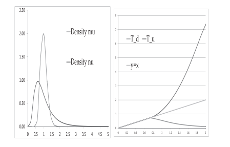
If $c$ is strictly monotone of order 2 , there exists a unique optimal transference plan for the $\mathrm{MK}{n}$ transport problem, and it has the form $$ \mathbb{P}^{*}\left(d s{1}, \ldots, d s_{n}\right)=\mathbb{P}^{1}\left(d s_{1}\right) \prod_{i=2}^{n} \delta_{T_{i}\left(s_{1}\right)}\left(d s_{i}\right), \quad T_{i}(s)=F_{i}^{-1} \circ F_{1}(s), i=2, \ldots, n
$$
The optimal upper bound is
$$
\mathrm{MK}{n}=\int c\left(x, T{2}(x), \ldots, T_{n}(x)\right) \mathbb{P}^{1}(d x)
$$
An extension to the infinite many marginals case has been obtained recently by Pass $[125]$ who studies
$$
\mathrm{MK}{\infty} \equiv \sup {\mathbb{P}: S_{\mathrm{t}} \sim \mathbb{P} t, \forall t \in(0, T]} \mathbb{E}\left[h\left(\int_{0}^{T} S_{t} d t\right)\right]
$$
where $h$ is a convex function. Let $F_{t}$ the cumulative distribution of $\mathbb{P}^{t}$. Define the stochastic process $S_{t}^{\text {opt }}(\omega)=F_{t}^{-1}(\omega), \quad \omega \in[0,1]$. The underlying probability space is the interval $[0,1]$ with Lebesgue measure.
统计代写|离散时间鞅理论代写martingale代考|Link with Hamilton-Jacobi equation
Here we take a cost function $c\left(s_{1}, s_{2}\right)=L\left(s_{2}-s_{1}\right)$ with $L$ a strictly concave function such that the Spence-Mirrlees condition is satisfied. From the formulation (2.8), one can link the Monge-Kantorovich formulation to the solution of a Hamilton-Jacobi equation through the Hopf-Lax formula:
PROPOSITION 2.3 see e.g. [139]
$$
\mathrm{MK}{2}=\inf {u(1, \cdot)}-\mathbb{E}^{\mathbb{P}^{1}}\left[u\left(0, S_{1}\right)\right]+\mathbb{E}^{\mathbb{P}^{2}}\left[u\left(1, S_{2}\right)\right]
$$
where $u(0, \cdot)$ is the (viscosity) solution at $t=0$ of the following HJ equation with terminal boundary condition $u(1,-):$
$$
\partial_{t} u+H(D u)=0, \quad H(p) \equiv \inf _{q}{p q-L(q)}
$$
PROOF From the dynamic programming principle, $u$, satisfying HamiltonJacobi equation (2.21), can be written as
$$
u(t, x)=\inf {\zeta} u\left(1, x+\int{t}^{1} \dot{\zeta}(s) d s\right)-\int_{t}^{1} L(\dot{\zeta}(s)) d s
$$
The minimisation over $\dot{\zeta}$ gives that $\dot{\zeta}$ is a constant $q$ (Fréchet derivative with respect to $\dot{\zeta}$ gives the critical equation $\left.\frac{d^{2} \zeta(t)}{d t^{2}}=0\right)$.
$$
u(t, x)=\inf {q} u(1, x+q(1-t))-L(q)(1-t) $$ By setting $y=x+q(1-t)$, we get Hopf-Lax’s formula: $$ u(t, x)=\inf {y} u(1, y)-L\left(\frac{y-x}{1-t}\right)(1-t)
$$
For $t=0$, this gives that $-u(0, \cdot)$ is the L-transform of $u(1, \cdot):-u(0, x)=$ $\sup _{y} L(y-x)-u(1, y)$. We conclude with Proposition 2.1.
In the next section, we introduce a martingale version of OT, first developed in $[17,77]$ where we have obtained a Monge-Kantorovich duality result.
统计代写|离散时间鞅理论代写martingale代考|Martingale optimal transport
We consider a payoff $c\left(s_{1}, s_{2}\right)$ depending on a single asset evaluated at two dates $t_{1}{2}$ : DEFINITION $2.5$ $$ \widetilde{\mathrm{MK}}{2} \equiv \inf {\mathcal{M}^{}\left(\mathbb{P}^{1}, \mathbb{P}^{2}\right)} \mathbb{E}^{\mathbb{P}^{1}}\left[\lambda{1}\left(S_{1}\right)\right]+\mathbb{E}^{\mathbb{P}^{2}}\left[\lambda_{2}\left(S_{2}\right)\right] $$ where $\mathcal{M}^{}\left(\mathbb{P}^{1}, \mathbb{P}^{2}\right)$ is the set of functions $\lambda_{1} \in \mathrm{L}^{1}\left(\mathbb{P}^{1}\right), \lambda_{2} \in \mathrm{L}^{1}\left(\mathbb{P}^{2}\right)$ and $H$ a bounded continuous function on $\mathbb{R}{+}$such that $$ \lambda{1}\left(s_{1}\right)+\lambda_{2}\left(s_{2}\right)+H\left(s_{1}\right)\left(s_{2}-s_{1}\right) \geq c\left(s_{1}, s_{2}\right), \quad \forall\left(s_{1}, s_{2}\right) \in \mathbb{R}{+}^{2} $$ This corresponds to a semi-static hedging strategy which consists in holding European payoffs $\lambda{1}$ and $\lambda_{2}$ and applying a delta strategy at $t_{1}$, generating a
$\mathrm{P} \& \mathrm{~L} H\left(s_{1}\right)\left(s_{2}-s_{1}\right)$ at $t_{2}$ with zero cost. We could also add a term $H_{0}\left(S_{0}\right)\left(s_{1}-\right.$ $\left.S_{0}\right)$ corresponding to performing a delta-hedging at $t=0$. As this term can be incorporated into $\lambda_{1}\left(s_{1}\right)$, it is not included. Similarly, an intermediate deltahedging term $H_{i}\left(S_{0}, \ldots, s_{t_{i}}\right)\left(s_{t_{i+1}}-s_{t_{i}}\right)$ where $0<t_{i}<t_{i+1} \leq t_{2}$ can be added but it can be shown that the optimal solution is attained for $H_{i}=0$. These terms are therefore not needed and will be disregarded next (see Corollary $2.1)$
Note that in comparison with the OT MK $\mathrm{MK}{2}$ previously reported, we have $\overline{\mathrm{MK}}{2} \leq \mathrm{MK}_{2}$ due to the appearance of the function $H$.
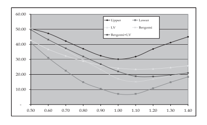
At this point, a natural question is how the classical results in OT generalize in the present martingale version. We follow closely our introduction of OT and explain how the various concepts previously explained extend to the present setting. Our research partly originates from a systematic derivation of Skorokhod embedding solutions and understanding of particle methods for non-linear McKean stochastic differential equations appearing in the calibration of financial models (see Section 4.2.4). From a practical point of view, the derivation of these optimal bounds allows to better understand the risk of exotic options as illustrated in the next example.
离散时间鞅理论代考
统计代写|离散时间鞅理论代写martingale代考|Multi-marginals and infinitely-many marginals case
大多数关于 OT 的文献都集中在具有回报的 2 资产案例上C(s1,s2). 对于数学金融中的应用,研究多资产收益的情况很有趣C(s1,…,sn)根据n在同一期限评估的资产。我们定义n-资产最优运输问题(通过对偶)为
米ķn≡支持磷∈磷(磷1,…,磷n)和磷[C(小号1,…,小号n)]
和\mathcal{P}\left(\mathbb{P}^{1}, \ldots, \mathbb{P}^{n}\right)=\left{\mathbb{P}: S_{i} \stackrel{ \mathbb{P}}{\sim} \mathbb{P}^{i}, \forall i=1, \ldots, n\right}\mathcal{P}\left(\mathbb{P}^{1}, \ldots, \mathbb{P}^{n}\right)=\left{\mathbb{P}: S_{i} \stackrel{ \mathbb{P}}{\sim} \mathbb{P}^{i}, \forall i=1, \ldots, n\right}. Gangbo [78] 和 Carlier [36] 最近已经研究了这个问题(另见 Pass [124]),对收益有以下要求:
定义2.4见[36]C∈C2如果对所有人来说是严格的 2 阶单调(一世,j)∈1,…,n2和一世≠j, 所有二阶导数∂一世jC是积极的。
我们有
定理2.4看[78,36]
如果C是严格单调的 2 阶,存在唯一的最优迁移计划米ķn运输问题,形式为
磷∗(ds1,…,dsn)=磷1(ds1)∏一世=2nd吨一世(s1)(ds一世),吨一世(s)=F一世−1∘F1(s),一世=2,…,n
最优上限是
米ķn=∫C(X,吨2(X),…,吨n(X))磷1(dX)
Pass 最近获得了对无限多边际情况的扩展[125]谁学习
米ķ∞≡支持磷:小号吨∼磷吨,∀吨∈(0,吨]和[H(∫0吨小号吨d吨)]
在哪里H是一个凸函数。让F吨的累积分布磷吨. 定义随机过程小号吨选择 (ω)=F吨−1(ω),ω∈[0,1]. 潜在的概率空间是区间[0,1]用勒贝格测度。
统计代写|离散时间鞅理论代写martingale代考|Link with Hamilton-Jacobi equation
这里我们取一个代价函数C(s1,s2)=大号(s2−s1)和大号满足 Spence-Mirrlees 条件的严格凹函数。从公式 (2.8),可以通过 Hopf-Lax 公式将 Monge-Kantorovich 公式与 Hamilton-Jacobi 方程的解联系起来:
命题 2.3 参见例如 [139]
米ķ2=信息在(1,⋅)−和磷1[在(0,小号1)]+和磷2[在(1,小号2)]
在哪里在(0,⋅)是(粘度)解决方案吨=0具有终端边界条件的以下 HJ 方程的在(1,−):
∂吨在+H(D在)=0,H(p)≡信息qpq−大号(q)
证明 从动态规划原理,在,满足 HamiltonJacobi 方程(2.21),可以写为
在(吨,X)=信息G在(1,X+∫吨1G˙(s)ds)−∫吨1大号(G˙(s))ds
最小化超过G˙给出了那个G˙是一个常数q(关于 Fréchet 导数G˙给出临界方程d2G(吨)d吨2=0).
在(吨,X)=信息q在(1,X+q(1−吨))−大号(q)(1−吨)通过设置是=X+q(1−吨),我们得到 Hopf-Lax 公式:
在(吨,X)=信息是在(1,是)−大号(是−X1−吨)(1−吨)
为了吨=0,这给出了−在(0,⋅)是的 L 变换在(1,⋅):−在(0,X)= 支持是大号(是−X)−在(1,是). 我们以命题 2.1 结束。
在下一节中,我们将介绍一个鞅版本的 OT,它首先在[17,77]我们得到了 Monge-Kantorovich 对偶结果。
统计代写|离散时间鞅理论代写martingale代考|Martingale optimal transport
我们认为有回报C(s1,s2)取决于在两个日期评估的单一资产吨12: 定义2.5
米ķ~2≡信息米(磷1,磷2)和磷1[λ1(小号1)]+和磷2[λ2(小号2)]在哪里米(磷1,磷2)是函数集λ1∈大号1(磷1),λ2∈大号1(磷2)和H一个有界连续函数R+这样
λ1(s1)+λ2(s2)+H(s1)(s2−s1)≥C(s1,s2),∀(s1,s2)∈R+2这对应于一种半静态对冲策略,包括持有欧洲收益λ1和λ2并在吨1,生成一个
磷& 大号H(s1)(s2−s1)在吨2零成本。我们还可以添加一个术语H0(小号0)(s1− 小号0)对应于在吨=0. 因为这个词可以并入λ1(s1), 不包括在内。类似地,一个中间 deltahedging 项H一世(小号0,…,s吨一世)(s吨一世+1−s吨一世)在哪里0<吨一世<吨一世+1≤吨2可以添加,但可以证明获得了最优解H一世=0. 因此,这些术语是不需要的,接下来将被忽略(参见推论2.1)
请注意,与 OT MK 相比米ķ2之前报道过,我们有米ķ¯2≤米ķ2由于函数的出现H.
在这一点上,一个自然的问题是 OT 中的经典结果如何在当前的鞅版本中推广。我们密切关注对 OT 的介绍,并解释先前解释的各种概念如何扩展到当前环境。我们的研究部分源于对 Skorokhod 嵌入解的系统推导和对金融模型校准中出现的非线性 McKean 随机微分方程的粒子方法的理解(参见第 4.2.4 节)。从实践的角度来看,这些最优界限的推导可以更好地理解奇异期权的风险,如下一个例子所示。

统计代写请认准statistics-lab™. statistics-lab™为您的留学生涯保驾护航。
金融工程代写
金融工程是使用数学技术来解决金融问题。金融工程使用计算机科学、统计学、经济学和应用数学领域的工具和知识来解决当前的金融问题,以及设计新的和创新的金融产品。
非参数统计代写
非参数统计指的是一种统计方法,其中不假设数据来自于由少数参数决定的规定模型;这种模型的例子包括正态分布模型和线性回归模型。
广义线性模型代考
广义线性模型(GLM)归属统计学领域,是一种应用灵活的线性回归模型。该模型允许因变量的偏差分布有除了正态分布之外的其它分布。
术语 广义线性模型(GLM)通常是指给定连续和/或分类预测因素的连续响应变量的常规线性回归模型。它包括多元线性回归,以及方差分析和方差分析(仅含固定效应)。
有限元方法代写
有限元方法(FEM)是一种流行的方法,用于数值解决工程和数学建模中出现的微分方程。典型的问题领域包括结构分析、传热、流体流动、质量运输和电磁势等传统领域。
有限元是一种通用的数值方法,用于解决两个或三个空间变量的偏微分方程(即一些边界值问题)。为了解决一个问题,有限元将一个大系统细分为更小、更简单的部分,称为有限元。这是通过在空间维度上的特定空间离散化来实现的,它是通过构建对象的网格来实现的:用于求解的数值域,它有有限数量的点。边界值问题的有限元方法表述最终导致一个代数方程组。该方法在域上对未知函数进行逼近。[1] 然后将模拟这些有限元的简单方程组合成一个更大的方程系统,以模拟整个问题。然后,有限元通过变化微积分使相关的误差函数最小化来逼近一个解决方案。
tatistics-lab作为专业的留学生服务机构,多年来已为美国、英国、加拿大、澳洲等留学热门地的学生提供专业的学术服务,包括但不限于Essay代写,Assignment代写,Dissertation代写,Report代写,小组作业代写,Proposal代写,Paper代写,Presentation代写,计算机作业代写,论文修改和润色,网课代做,exam代考等等。写作范围涵盖高中,本科,研究生等海外留学全阶段,辐射金融,经济学,会计学,审计学,管理学等全球99%专业科目。写作团队既有专业英语母语作者,也有海外名校硕博留学生,每位写作老师都拥有过硬的语言能力,专业的学科背景和学术写作经验。我们承诺100%原创,100%专业,100%准时,100%满意。
随机分析代写
随机微积分是数学的一个分支,对随机过程进行操作。它允许为随机过程的积分定义一个关于随机过程的一致的积分理论。这个领域是由日本数学家伊藤清在第二次世界大战期间创建并开始的。
时间序列分析代写
随机过程,是依赖于参数的一组随机变量的全体,参数通常是时间。 随机变量是随机现象的数量表现,其时间序列是一组按照时间发生先后顺序进行排列的数据点序列。通常一组时间序列的时间间隔为一恒定值(如1秒,5分钟,12小时,7天,1年),因此时间序列可以作为离散时间数据进行分析处理。研究时间序列数据的意义在于现实中,往往需要研究某个事物其随时间发展变化的规律。这就需要通过研究该事物过去发展的历史记录,以得到其自身发展的规律。
回归分析代写
多元回归分析渐进(Multiple Regression Analysis Asymptotics)属于计量经济学领域,主要是一种数学上的统计分析方法,可以分析复杂情况下各影响因素的数学关系,在自然科学、社会和经济学等多个领域内应用广泛。
MATLAB代写
MATLAB 是一种用于技术计算的高性能语言。它将计算、可视化和编程集成在一个易于使用的环境中,其中问题和解决方案以熟悉的数学符号表示。典型用途包括:数学和计算算法开发建模、仿真和原型制作数据分析、探索和可视化科学和工程图形应用程序开发,包括图形用户界面构建MATLAB 是一个交互式系统,其基本数据元素是一个不需要维度的数组。这使您可以解决许多技术计算问题,尤其是那些具有矩阵和向量公式的问题,而只需用 C 或 Fortran 等标量非交互式语言编写程序所需的时间的一小部分。MATLAB 名称代表矩阵实验室。MATLAB 最初的编写目的是提供对由 LINPACK 和 EISPACK 项目开发的矩阵软件的轻松访问,这两个项目共同代表了矩阵计算软件的最新技术。MATLAB 经过多年的发展,得到了许多用户的投入。在大学环境中,它是数学、工程和科学入门和高级课程的标准教学工具。在工业领域,MATLAB 是高效研究、开发和分析的首选工具。MATLAB 具有一系列称为工具箱的特定于应用程序的解决方案。对于大多数 MATLAB 用户来说非常重要,工具箱允许您学习和应用专业技术。工具箱是 MATLAB 函数(M 文件)的综合集合,可扩展 MATLAB 环境以解决特定类别的问题。可用工具箱的领域包括信号处理、控制系统、神经网络、模糊逻辑、小波、仿真等。