如果你也在 怎样代写风险理论投资组合这个学科遇到相关的难题,请随时右上角联系我们的24/7代写客服。
为了衡量市场风险,投资者和分析师使用风险值(VaR)方法。风险值建模是一种统计风险管理方法,它可以量化股票或投资组合的潜在损失,以及该潜在损失发生的概率。
statistics-lab™ 为您的留学生涯保驾护航 在代写风险理论投资组合方面已经树立了自己的口碑, 保证靠谱, 高质且原创的统计Statistics代写服务。我们的专家在代写风险理论投资组合代写方面经验极为丰富,各种代写风险理论投资组合相关的作业也就用不着说。
我们提供的风险理论投资组合及其相关学科的代写,服务范围广, 其中包括但不限于:
- Statistical Inference 统计推断
- Statistical Computing 统计计算
- Advanced Probability Theory 高等概率论
- Advanced Mathematical Statistics 高等数理统计学
- (Generalized) Linear Models 广义线性模型
- Statistical Machine Learning 统计机器学习
- Longitudinal Data Analysis 纵向数据分析
- Foundations of Data Science 数据科学基础
金融代写|风险理论投资组合代写Market Risk, Measures and Portfolio 代考|Probability Distribution Function, Probability
If the random variable can take on any possible value within the range of outcomes, then the probability distribution is said to be a contimuous random variable. ${ }^{7}$ When a random variable is either the price of or the return on a financial asset or an interest rate, the random variable is assumed to be continuous. This means that it is possible to obtain, for example, a price of $95.43231$ or $109.34872$ and any value in between. In practice, we know that financial assets are not quoted in such a way. Nevertheless, there is no loss in describing the random variable as continuous and in many times treating the return as a continuous random variable means substantial gain in mathematical tractability and convenience. For a continuous random variable, the calculation of probabilities is substantially different from the discrete case. The reason is that if we want to derive the probability that the realization of the random variable lays within some range (i.e., over a subset or subinterval of the sample space), then we cannot proceed in a similar way as in the discrete case: The number of values in an interval is so large, that we cannot just add the probabilities of the single outcomes. The new concept needed is explained in the next section.
A probability distribution function $P$ assigns a probability $P(A)$ for every event $A$, that is, of realizing a value for the random value in any specified subset $A$ of the sample space. For example, a probability distribution function can assign a probability of realizing a monthly return that is negative or the probability of realizing a monthly return that is greater than $0.5 \%$ or the probability of realizing a monthly return that is between $0.4 \%$ and $1.0 \%$
To compute the probability, a mathematical function is needed to represent the probability distribution function. There are several possibilities of representing a probability distribution by means of a mathematical function. In the case of a continuous probability distribution, the most popular way is to provide the so-called probability density function or simply density function.
In general, we denote the density function for the random variable $X$ as $f_{X}(x)$. Note that the letter $x$ is used for the function argument and the index denotes that the density function corresponds to the random variable $X$. The letter $x$ is the convention adopted to denote a particular value for the random variable. The density function of a probability distribution is always nonnegative and as its name indicates: Large values for $f_{X}(x)$ of the density function at some point $x$ imply a relatively high probability of realizing a value in the neighborhood of $x$, whereas $f_{X}(x)=0$ for all $x$ in some interval $(a, b)$ implies that the probability for observing a realization in $(a, b)$ is zero.
Figure $1.1$ aids in understanding a continuous probability distribution. The shaded area is the probability of realizing a return less than $b$ and greater than $a$. As probabilities are represented by areas under the density function, it follows that the probability for every single outcome of a continuous random variable always equals zero. While the shaded area
in Figure $1.1$ represents the probability associated with realizing a return within the specified range, how does one compute the probability? This is where the tools of calculus are applied. Calculus involves differentiation and integration of a mathematical function. The latter tool is called integral calculus and involves computing the area under a curve. Thus the probability that a realization from a random variable is between two real numbers $a$ and $b$ is calculated according to the formula,
$$
P(a \leq X \leq b)=\int_{a}^{b} f_{X}(x) d x
$$
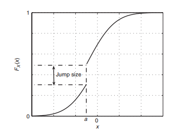
The mathematical function that provides the cumulative probability of a probability distribution, that is, the function that assigns to every real value $x$ the probability of getting an outcome less than or equal to $x$, is called the cumulative distribution function or cumulative probability function or simply distribution function and is denoted mathematically by $F_{X}(x)$. A cumulative distribution function is always nonnegative, nondecreasing, and as it represents probabilities it takes only values between zero and one. ${ }^{8} \mathrm{An}$ example of a distribution function is given in Figure 1.2.
金融代写|风险理论投资组合代写Market Risk, Measures and Portfolio 代考|The Normal Distribution
The class of normal distributions, or Gaussian distributions, is certainly one of the most important probability distributions in statistics and due to some of its appealing properties also the class which is used in most applications in finance. Here we introduce some of its basic properties.
The random variable $X$ is said to be normally distributed with parameters $\mu$ and $\sigma$, abbreviated by $X \in N\left(\mu, \sigma^{2}\right)$, if the density of the random
$$
f_{X}(x)=\frac{1}{\sqrt{2 \pi \sigma^{2}}} e^{-\frac{(x-\mu)^{2}}{2 \sigma^{2}}}, x \in \mathbb{R} \text {. }
$$
The parameter $\mu$ is called a location parameter because the middle of the distribution equals $\mu$ and $\sigma$ is called a shape parameter or a scale parameter. If $\mu=0$ and $\sigma=1$, then $X$ is said to have a standard normal distribution.
An important property of the normal distribution is the location-scale invariance of the normal distribution. What does this mean? Imagine you have random variable $X$, which is normally distributed with the parameters $\mu$ and $\sigma$. Now we consider the random variable $Y$, which is obtained as $Y=$ $a X+b .$ In general, the distribution of $Y$ might substantially differ from the distribution of $X$ but in the case where $X$ is normally distributed, the random variable $Y$ is again normally distributed with parameters and $\bar{\mu}=a \mu+b$ and $\bar{\sigma}=a \sigma$. Thus we do not leave the class of normal distributions if we multiply the random variable by a factor or shift the random variable. This fact can be used if we change the scale where a random variable is measured: Imagine that $X$ measures the temperature at the top of the Empire State Building on January 1, 2008, at 6 A.M. in degrees Celsius. Then $Y=\frac{9}{5} X+32$ will give the temperature in degrees Fahrenheit, and if $X$ is normally distributed, then $Y$ will be too.
金融代写|风险理论投资组合代写Market Risk, Measures and Portfolio 代考|Exponential Distribution
The exponential distribution is popular, for example, in queuing theory when we want to model the time we have to wait until a certain event takes place. Examples include the time until the next client enters the store, the time until a certain company defaults or the time until some machine has a defect.
As it is used to model waiting times, the exponential distribution is concentrated on the positive real numbers and the density function $f$ and the cumulative distribution function $F$ of an exponentially distributed random variable $\tau$ possess the following form:
$$
f_{\mathrm{r}}(x)=\frac{1}{\beta} e^{-\frac{x}{\beta}}, x>0
$$
and
$$
F_{\mathrm{r}}(x)=1-e^{-\frac{x}{\beta}}, x>0 .
$$
In credit risk modeling, the parameter $\lambda=1 / \beta$ has a natural interpretation as hazard rate or default intensity. Let $\tau$ denote an exponential distributed random variable, for example, the random time (counted in days and started on January 1, 2008) we have to wait until Ford Motor Company defaults. Now, consider the following expression:
$$
\lambda(\Delta t)=\frac{P(\tau \in(t, t+\Delta t] \mid \tau>t)}{\Delta t}=\frac{P(\tau \in(t, t+\Delta t])}{\Delta t P(\tau>t)} .
$$
where $\Delta t$ denotes a small period of time.
What is the interpretation of this expression? $\lambda(\Delta t)$ represents a ratio of a probability and the quantity $\Delta t$. The probability in the numerator represents the probability that default occurs in the time interval $(t, t+\Delta t]$ conditional upon the fact that Ford Motor Company survives until time $t$. The notion of conditional probability is explained in section 1.6.1.
Now the ratio of this probability and the length of the considered time interval can be denoted as a default rate or default intensity. In applications different from credit risk we also use the expressions hazard or failure rate.
Now, letting $\Delta t$ tend to zero we finally obtain after some calculus the desired relation $\lambda=1 / \beta$. What we can see is that in the case of an exponentially distributed time of default, we are faced with a constant rate of default that is independent of the current point in time $t$.
Another interesting fact linked to the exponential distribution is the following connection with the Poisson distribution described earlier. Consider a sequence of independent and identical exponentially distributed random variables $\tau_{1}, \tau_{2}, \ldots$ We can think of $\tau_{1}$, for example, as the time we have to wait until a firm in a high-yield bond portfolio defaults. $\tau_{2}$ will then represent the time between the first and the second default and so on. These waiting times are sometimes called interarrival times. Now, let $N_{t}$ denote the number of defaults which have occurred until time $t \geq 0$. One important probabilistic result states that the random variable $N_{t}$ is Poisson distributed with parameter $\lambda=t / \beta$.
风险理论投资组合代写
金融代写|风险理论投资组合代写Market Risk, Measures and Portfolio 代考|Probability Distribution Function, Probability
如果随机变量可以取结果范围内的任何可能值,则称概率分布为连续随机变量。7当随机变量是金融资产的价格或收益或利率时,假设随机变量是连续的。这意味着有可能获得,例如,价格为95.43231或者109.34872以及介于两者之间的任何值。在实践中,我们知道金融资产不会以这种方式报价。尽管如此,将随机变量描述为连续的并没有损失,并且在很多时候将收益视为连续的随机变量意味着在数学易处理性和便利性方面的实质性收益。对于连续随机变量,概率的计算与离散情况有很大不同。原因是,如果我们想推导出随机变量的实现位于某个范围内(即,在样本空间的子集或子区间上)的概率,那么我们不能以与离散情况类似的方式进行:一个区间中的值的数量是如此之大,以至于我们不能只添加单个结果的概率。下一节将解释所需的新概念。
概率分布函数磷分配一个概率磷(一种)对于每一个事件一种,即在任何指定子集中实现随机值的值一种的样本空间。例如,概率分布函数可以分配实现月收益为负的概率或实现月收益的概率大于0.5%或实现每月回报的概率介于0.4%和1.0%
为了计算概率,需要一个数学函数来表示概率分布函数。通过数学函数表示概率分布有几种可能性。在连续概率分布的情况下,最流行的方式是提供所谓的概率密度函数或简称为密度函数。
通常,我们表示随机变量的密度函数X作为FX(X). 请注意,这封信X用于函数参数,索引表示密度函数对应于随机变量X. 信X是为表示随机变量的特定值而采用的约定。概率分布的密度函数总是非负的,正如其名称所示:FX(X)某点的密度函数X意味着在附近实现价值的概率相对较高X, 然而FX(X)=0对全部X在某个区间(一种,b)意味着观察到实现的概率(一种,b)为零。
数字1.1有助于理解连续概率分布。阴影区域是实现回报的概率小于b并且大于一种. 由于概率由密度函数下的面积表示,因此连续随机变量的每个单个结果的概率始终为零。而阴影区域
如图1.1表示在指定范围内实现回报的概率,如何计算概率?这是应用微积分工具的地方。微积分涉及数学函数的微分和积分。后一种工具称为积分学,涉及计算曲线下的面积。因此,随机变量的实现在两个实数之间的概率一种和b根据公式计算,
磷(一种≤X≤b)=∫一种bFX(X)dX
提供概率分布的累积概率的数学函数,即分配给每个实数值的函数X得到结果的概率小于或等于X, 称为累积分布函数或累积概率函数或简称分布函数,在数学上表示为FX(X). 累积分布函数始终是非负的、非递减的,并且因为它表示概率,它只取零和一之间的值。8一种n图 1.2 给出了分布函数的例子。
金融代写|风险理论投资组合代写Market Risk, Measures and Portfolio 代考|The Normal Distribution
正态分布或高斯分布类无疑是统计学中最重要的概率分布之一,并且由于其一些吸引人的特性,它也是金融领域大多数应用中使用的类。下面我们介绍一下它的一些基本属性。
随机变量X据说与参数正态分布μ和σ, 缩写为X∈ñ(μ,σ2),如果随机的密度FX(X)=12圆周率σ2和−(X−μ)22σ2,X∈R.
参数μ被称为位置参数,因为分布的中间等于μ和σ称为形状参数或比例参数。如果μ=0和σ=1, 然后X据说服从标准正态分布。
正态分布的一个重要性质是正态分布的位置尺度不变性。这是什么意思?想象一下你有随机变量X, 它与参数呈正态分布μ和σ. 现在我们考虑随机变量是,得到为是= 一种X+b.一般来说,分布是可能与分布有很大不同X但在这种情况下X是正态分布的,随机变量是再次正态分布,参数和μ¯=一种μ+b和σ¯=一种σ. 因此,如果我们将随机变量乘以一个因子或移动随机变量,我们不会离开正态分布的类别。如果我们改变测量随机变量的尺度,则可以使用这个事实:想象一下X测量 2008 年 1 月 1 日早上 6 点帝国大厦顶部的温度(以摄氏度为单位)。然后是=95X+32将以华氏度为单位给出温度,如果X是正态分布的,那么是也会。
金融代写|风险理论投资组合代写Market Risk, Measures and Portfolio 代考|Exponential Distribution
指数分布很流行,例如,在排队论中,当我们想要模拟我们必须等到某个事件发生的时间时。示例包括直到下一个客户进入商店的时间、直到某个公司违约的时间或直到某些机器出现缺陷的时间。
由于它用于模拟等待时间,指数分布集中在正实数和密度函数上F和累积分布函数F指数分布的随机变量τ具有以下形式:
Fr(X)=1b和−Xb,X>0
和
Fr(X)=1−和−Xb,X>0.
在信用风险建模中,参数λ=1/b自然解释为风险率或违约强度。让τ表示一个指数分布的随机变量,例如,我们必须等到福特汽车公司违约的随机时间(以天计,从 2008 年 1 月 1 日开始)。现在,考虑以下表达式:
λ(Δ吨)=磷(τ∈(吨,吨+Δ吨]∣τ>吨)Δ吨=磷(τ∈(吨,吨+Δ吨])Δ吨磷(τ>吨).
在哪里Δ吨表示一小段时间。
这个表达的解释是什么?λ(Δ吨)表示概率与数量的比值Δ吨. 分子中的概率表示该时间区间内发生违约的概率(吨,吨+Δ吨]条件是福特汽车公司能够生存到时间吨. 条件概率的概念在 1.6.1 节中解释。
现在,这个概率与所考虑的时间间隔的长度之比可以表示为违约率或违约强度。在与信用风险不同的应用中,我们也使用表达风险或故障率。
现在,让Δ吨趋于零我们最终在一些微积分之后获得所需的关系λ=1/b. 我们可以看到,在违约时间呈指数分布的情况下,我们面临着与当前时间点无关的恒定违约率吨.
与指数分布相关的另一个有趣事实是与前面描述的泊松分布的以下联系。考虑一系列独立且相同的指数分布随机变量τ1,τ2,…我们可以想到τ1,例如,作为我们必须等到某个公司在高收益债券投资组合中违约的时间。τ2然后将表示第一个和第二个默认值之间的时间,依此类推。这些等待时间有时称为到达间隔时间。现在,让ñ吨表示直到时间发生的默认值的数量吨≥0. 一个重要的概率结果表明,随机变量ñ吨是带参数的泊松分布λ=吨/b.

统计代写请认准statistics-lab™. statistics-lab™为您的留学生涯保驾护航。
金融工程代写
金融工程是使用数学技术来解决金融问题。金融工程使用计算机科学、统计学、经济学和应用数学领域的工具和知识来解决当前的金融问题,以及设计新的和创新的金融产品。
非参数统计代写
非参数统计指的是一种统计方法,其中不假设数据来自于由少数参数决定的规定模型;这种模型的例子包括正态分布模型和线性回归模型。
广义线性模型代考
广义线性模型(GLM)归属统计学领域,是一种应用灵活的线性回归模型。该模型允许因变量的偏差分布有除了正态分布之外的其它分布。
术语 广义线性模型(GLM)通常是指给定连续和/或分类预测因素的连续响应变量的常规线性回归模型。它包括多元线性回归,以及方差分析和方差分析(仅含固定效应)。
有限元方法代写
有限元方法(FEM)是一种流行的方法,用于数值解决工程和数学建模中出现的微分方程。典型的问题领域包括结构分析、传热、流体流动、质量运输和电磁势等传统领域。
有限元是一种通用的数值方法,用于解决两个或三个空间变量的偏微分方程(即一些边界值问题)。为了解决一个问题,有限元将一个大系统细分为更小、更简单的部分,称为有限元。这是通过在空间维度上的特定空间离散化来实现的,它是通过构建对象的网格来实现的:用于求解的数值域,它有有限数量的点。边界值问题的有限元方法表述最终导致一个代数方程组。该方法在域上对未知函数进行逼近。[1] 然后将模拟这些有限元的简单方程组合成一个更大的方程系统,以模拟整个问题。然后,有限元通过变化微积分使相关的误差函数最小化来逼近一个解决方案。
tatistics-lab作为专业的留学生服务机构,多年来已为美国、英国、加拿大、澳洲等留学热门地的学生提供专业的学术服务,包括但不限于Essay代写,Assignment代写,Dissertation代写,Report代写,小组作业代写,Proposal代写,Paper代写,Presentation代写,计算机作业代写,论文修改和润色,网课代做,exam代考等等。写作范围涵盖高中,本科,研究生等海外留学全阶段,辐射金融,经济学,会计学,审计学,管理学等全球99%专业科目。写作团队既有专业英语母语作者,也有海外名校硕博留学生,每位写作老师都拥有过硬的语言能力,专业的学科背景和学术写作经验。我们承诺100%原创,100%专业,100%准时,100%满意。
随机分析代写
随机微积分是数学的一个分支,对随机过程进行操作。它允许为随机过程的积分定义一个关于随机过程的一致的积分理论。这个领域是由日本数学家伊藤清在第二次世界大战期间创建并开始的。
时间序列分析代写
随机过程,是依赖于参数的一组随机变量的全体,参数通常是时间。 随机变量是随机现象的数量表现,其时间序列是一组按照时间发生先后顺序进行排列的数据点序列。通常一组时间序列的时间间隔为一恒定值(如1秒,5分钟,12小时,7天,1年),因此时间序列可以作为离散时间数据进行分析处理。研究时间序列数据的意义在于现实中,往往需要研究某个事物其随时间发展变化的规律。这就需要通过研究该事物过去发展的历史记录,以得到其自身发展的规律。
回归分析代写
多元回归分析渐进(Multiple Regression Analysis Asymptotics)属于计量经济学领域,主要是一种数学上的统计分析方法,可以分析复杂情况下各影响因素的数学关系,在自然科学、社会和经济学等多个领域内应用广泛。
MATLAB代写
MATLAB 是一种用于技术计算的高性能语言。它将计算、可视化和编程集成在一个易于使用的环境中,其中问题和解决方案以熟悉的数学符号表示。典型用途包括:数学和计算算法开发建模、仿真和原型制作数据分析、探索和可视化科学和工程图形应用程序开发,包括图形用户界面构建MATLAB 是一个交互式系统,其基本数据元素是一个不需要维度的数组。这使您可以解决许多技术计算问题,尤其是那些具有矩阵和向量公式的问题,而只需用 C 或 Fortran 等标量非交互式语言编写程序所需的时间的一小部分。MATLAB 名称代表矩阵实验室。MATLAB 最初的编写目的是提供对由 LINPACK 和 EISPACK 项目开发的矩阵软件的轻松访问,这两个项目共同代表了矩阵计算软件的最新技术。MATLAB 经过多年的发展,得到了许多用户的投入。在大学环境中,它是数学、工程和科学入门和高级课程的标准教学工具。在工业领域,MATLAB 是高效研究、开发和分析的首选工具。MATLAB 具有一系列称为工具箱的特定于应用程序的解决方案。对于大多数 MATLAB 用户来说非常重要,工具箱允许您学习和应用专业技术。工具箱是 MATLAB 函数(M 文件)的综合集合,可扩展 MATLAB 环境以解决特定类别的问题。可用工具箱的领域包括信号处理、控制系统、神经网络、模糊逻辑、小波、仿真等。