如果你也在 怎样代写理论力学theoretical mechanics这个学科遇到相关的难题,请随时右上角联系我们的24/7代写客服。
理论力学主要研究物体的力学性能及运动规律,是力学的基础学科,由静力学、运动学和动力学三大部分组成。也有人认为运动学是动力学的一部分,而提出二分法。
statistics-lab™ 为您的留学生涯保驾护航 在代写理论力学theoretical mechanics方面已经树立了自己的口碑, 保证靠谱, 高质且原创的统计Statistics代写服务。我们的专家在代写理论力学theoretical mechanics代写方面经验极为丰富,各种代写理论力学theoretical mechanics相关的作业也就用不着说。
我们提供的理论力学theoretical mechanics及其相关学科的代写,服务范围广, 其中包括但不限于:
- Statistical Inference 统计推断
- Statistical Computing 统计计算
- Advanced Probability Theory 高等概率论
- Advanced Mathematical Statistics 高等数理统计学
- (Generalized) Linear Models 广义线性模型
- Statistical Machine Learning 统计机器学习
- Longitudinal Data Analysis 纵向数据分析
- Foundations of Data Science 数据科学基础
物理代写|理论力学代写theoretical mechanics代考|Solution of the System of Governing Equations
Solution of the system of Eq. (9) under conditions (10) can be constructed using the method of Chebyshev orthogonal polynomials, by reducing it to a quasi-completely regular system of algebraic equations [9]. However, more effective, in our opinion, is the method of mechanical quadratures [10], which we will use. Without loss of generality, we will assume that there is one crack and one inclusion in the base cell, which occupy intervals $(a, b)$ and $(c, d)$.
Turning to dimensionless quantities and introducing the notation
$$
\begin{aligned}
&a_{}=(b-a) / 2 h ; \quad b_{}=(b+a) / 2 h ; \quad c_{}=(d-c) / 2 h ; \quad d_{}=(d+c) / 2 h \
&\varphi_{1}(t)=V^{\prime}\left(h\left(a_{} t+b_{}\right)\right) ; \quad \varphi_{2}(t)=\frac{c_{} \tau\left(h\left(c_{} t+d_{}\right)\right)}{\mu_{1}} ; \ &R_{11}^{}(t, \xi)=\frac{a_{}}{\lambda_{1}} \int_{0}^{\infty} K_{11}(\zeta) \sin \left(\zeta a_{}(t-\xi)\right) d \zeta_{0} \
&R_{12}^{}(t, \xi)=\left(1-v_{1}\right) \int_{0}^{\infty} K_{12}(\zeta) \sin \left(\zeta\left(a_{} t+b_{}-c_{} \xi-d_{}\right)\right) d \zeta \ &R_{21}^{}(t, \xi)=-\frac{4 a_{} c_{}\left(1-v_{2}\right)}{\mu_{} K_{2}} \int_{0}^{\infty} K_{21}(\zeta) \sin \left(\zeta\left(c_{} t+d_{}-a_{} \xi-b_{}\right)\right) d \zeta \ &R_{22}^{}(t, \xi)=-\frac{c_{}}{\lambda_{2}} \int_{0}^{\infty} K_{22}(\zeta) \sin \left(\zeta c_{}(t-\xi)\right) d \zeta \
&f_{1}(t)=-\pi p_{1}\left[h\left(a_{} t+b_{}\right)\right] / \lambda_{1} ; \quad f_{2}(t)=\frac{2 \pi c_{} q_{2}\left(1-v_{2}^{2}\right)}{\mathbb{X}{2} \mu{1}} ; \
&P_{0}^{}=\frac{P_{0}^{(1)}}{h \mu_{1}} ; \quad \vartheta_{}=\frac{2 \pi h\left(1-v_{2}\right) c_{} E_{2}}{h_{1} E_{l}^{(1)}\left(1+v_{2}\right) \mathbb{T}{2}}, \end{aligned} $$ we obtain the following system of defining equations: under conditions $$ \int{-1}^{1} \varphi_{1}(s) d s=0 ; \quad \int_{-1}^{1} \varphi_{2}(s) d s=\frac{P_{0}^{*}}{2}
$$
物理代写|理论力学代写theoretical mechanics代考|Numerical Analysis
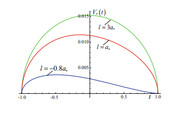
The numerical analysis is conducted based on the formulas of the preceding paragraph. It is assumed that the crack has a constant length equal to a quarter of the half-thickness of the layer $h$, and is located symmetrically about the axis $O y$, i.e. $a_{}=0.25, b_{}=0$. The location of the inclusion, whose length is equal to the length of the crack, can vary and is determined by the parameter $l$, which is the coordinate of the left end of the inclusion, i.e. $c_{}=a_{}, d_{}=l+a_{}$. In order to determine the effect of inclusion on the crack opening and on stress intensity factors (SIF) at its ends, we take the forces acting on the crack faces and the forces at infinity equal to zero $\left(p_{1}=0, q_{2}=0\right)$. The force applied to the left end of the inclusion $\left(t_{0}=-1\right)$, the ratio of the thickness of the inclusion to the half-thickness of the layer and the ratio of the Young’s modulus of the stringer to $E_{2}$ will be considered constants with values: $P_{0}^{*}=0.25, h_{1} / h=0.01, E_{I}^{(1)} / E_{2}=5$.
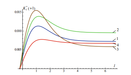
The calculations show that crack opens only when inclusion is located to the right of certain point, in other cases part of the crack is closed and the formulation of the problem is not valid. Note that the crack begins to close from the right end. The location of the above mentioned point can be found by equating the SIF at the right end of the crack to zero and it essentially depends only on the length of the inclusion. So, for example, if the inclusion length is equal to $a_{}$, this point is in the vicinity of the point $-0.8 a_{}$. If the inclusion length is equal to $2 a_{}$ the point is around $-2.4 a_{}$, and if the inclusion length is $0.5 a_{}$ the point is around $-0.1 a_{}$. Figure 2 shows the graphs of SIF at the right end of the crack depending on parameter $l$ for different values of the elastic constants of layers.
In Fig. 2, curve 1 corresponds to a homogeneous layer with $v_{1}=v_{2}=0.25$, curves $2,3,4$ correspond to inhomogeneous layers with parameters $E_{1} / E_{2}=1$,$v_{1}=0.25, v_{2}=0.35 ; E_{1} / E_{2}=3, v_{1}=v_{2}=0.25$ and $E_{1} / E_{2}=1 / 3, v_{1}=$ $0.25, v_{2}=0.35$ respectively.
物理代写|理论力学代写theoretical mechanics代考|Applied Instrumentation
We use two industrial US flaw detectors USD60-N and UD9812, shown in Fig. $2 .$ The low-frequency flaw detector USD60-N permits measurements in the frequency range $0.02-2.5 \mathrm{MHz}$ in the two regimes-the through-transmission method and echomethod. There is a possibility to display the full signal, the detected signal, as well as its spectrum. The second flaw detector UD9812 has the working frequency range $0.6-12 \mathrm{M \Gamma} ц$, and we use it to perform measurements at frequencies higher than $2.5 \mathrm{MHz}$. The both flaw detectors permit the transmission of the recorded data to a PC with the help of a special software. In the case of USD60-N for this aim one can use the network interface Ethernet, while the UD9812 can be attached to the PC with a USB 2.0.
As the generator and the receiver of US signals we use available US transducers of various frequencies and diameters.
Let us note that the values reflected in Table 1 are related to the maximum working frequency of the US transducer, while the spectrum generated by the probe contains a set of frequencies around the indicated carrier frequency. The measurements are
carried out by the through-transmitted method, when the radiating probe is placed on the top of the sample and another probe – on its bottom. To provide a good contact, we used a lubricating layer which permits the transition of the mechanical oscillations of the piezo-element inside the specimen at hand (Fig. 3).
A laboratory setup has been equipped to provide the experiments, see Fig. 4 , which is a device to fix the US probes and the sample. The device is a rack with three clamps. The first two clamps fix the receiving and radiated US transducers, between them there is a fixed sample for measurements, the third clamp fixes a spring which provides reliable contact between the transducers and the sample.
All experiments were performed without any additional amplifier with a fixed amplitude of $50 \mathrm{~V}$. The following filtration bands was applied to the received signal: at the frequency up to $0.2 \mathrm{MHz}$ we used a filtration over the interval $20-300 \mathrm{kHz}$; for the frequencies $0.4$ and $0.6 \mathrm{MHz}$ we put the filtration for the receiver $200-1250 \mathrm{kHz}$; the frequencies $1.25,1.8,2.5 \mathrm{MHz}$ were measured in the pass band $400-2500 \mathrm{kHz}$ for the frequencies 5 and $10 \mathrm{MHz}$-the frequency band $0.8-12 \mathrm{MHz}$.
理论力学代考
物理代写|理论力学代写theoretical mechanics代考|Solution of the System of Governing Equations
方程系统的解决方案。(9) 在条件 (10) 下,可以使用切比雪夫正交多项式的方法构造,通过将其简化为代数方程的准完全正则系统 [9]。然而,在我们看来,更有效的是我们将使用的机械求积法 [10]。不失一般性,我们假设基胞中存在1个裂缝和1个夹杂物,它们占据区间(一个,b)和(C,d).
转向无量纲量并引入符号
一个=(b−一个)/2H;b=(b+一个)/2H;C=(d−C)/2H;d=(d+C)/2H 披1(吨)=在′(H(一个吨+b));披2(吨)=Cτ(H(C吨+d))μ1; R11(吨,X)=一个λ1∫0∞ķ11(G)罪(G一个(吨−X))dG0 R12(吨,X)=(1−在1)∫0∞ķ12(G)罪(G(一个吨+b−CX−d))dG R21(吨,X)=−4一个C(1−在2)μķ2∫0∞ķ21(G)罪(G(C吨+d−一个X−b))dG R22(吨,X)=−Cλ2∫0∞ķ22(G)罪(GC(吨−X))dG F1(吨)=−圆周率p1[H(一个吨+b)]/λ1;F2(吨)=2圆周率Cq2(1−在22)X2μ1; 磷0=磷0(1)Hμ1;ϑ=2圆周率H(1−在2)C和2H1和l(1)(1+在2)吨2,我们得到以下定义方程的系统: 在条件下
∫−11披1(s)ds=0;∫−11披2(s)ds=磷0∗2
物理代写|理论力学代写theoretical mechanics代考|Numerical Analysis
数值分析是根据上一段的公式进行的。假设裂纹具有恒定长度,等于层半厚度的四分之一H, 并且关于轴对称地定位○是, IE一个=0.25,b=0. 夹杂物的位置,其长度等于裂纹的长度,可以变化,由参数决定l,即包含物左端的坐标,即C=一个,d=l+一个. 为了确定夹杂物对裂纹开口及其末端应力强度因子 (SIF) 的影响,我们将作用在裂纹面上的力和无穷远处的力设为零(p1=0,q2=0). 施加在夹杂物左端的力(吨0=−1),夹杂物的厚度与层的半厚度之比和纵梁的杨氏模量与和2将被视为具有值的常量:磷0∗=0.25,H1/H=0.01,和我(1)/和2=5.
计算表明,只有当夹杂物位于某个点的右侧时,裂缝才会打开,而在其他情况下,裂缝的一部分是闭合的,问题的表述是无效的。请注意,裂缝从右端开始闭合。上述点的位置可以通过将裂缝右端的 SIF 等于零来找到,它基本上只取决于夹杂物的长度。因此,例如,如果包含长度等于一个, 该点在该点附近−0.8一个. 如果包含长度等于2一个重点在附近−2.4一个, 如果包含长度是0.5一个重点在附近−0.1一个. 图 2 显示了裂缝右端 SIF 随参数变化的曲线图l对于层的弹性常数的不同值。
在图 2 中,曲线 1 对应于同质层在1=在2=0.25, 曲线2,3,4对应于带参数的非均匀层和1/和2=1,在1=0.25,在2=0.35;和1/和2=3,在1=在2=0.25和和1/和2=1/3,在1= 0.25,在2=0.35分别。
物理代写|理论力学代写theoretical mechanics代考|Applied Instrumentation
我们使用两个工业美国探伤仪 USD60-N 和 UD9812,如图 1 所示。2.低频探伤仪 USD60-N 允许在频率范围内进行测量0.02−2.5米H和在两种方案中——透传法和回声法。可以显示完整信号、检测到的信号及其频谱。二次探伤仪UD9812工作频率范围ц0.6−12米Γц, 我们用它在高于2.5米H和. 两个探伤仪都允许在特殊软件的帮助下将记录的数据传输到 PC。在 USD60-N 的情况下,可以使用网络接口以太网,而 UD9812 可以通过 USB 2.0 连接到 PC。
作为美国信号的发生器和接收器,我们使用各种频率和直径的可用美国传感器。
请注意,表 1 中反映的值与美国换能器的最大工作频率有关,而探头产生的频谱包含一组指定载波频率附近的频率。测量结果是
当辐射探头放在样品的顶部,另一个探头放在样品的底部时,通过透射法进行。为了提供良好的接触,我们使用了一个润滑层,它允许手头试样内部压电元件的机械振动发生转变(图 3)。
已经配备了一个实验室装置来提供实验,见图4,这是一个固定美国探针和样品的装置。该设备是一个带有三个夹子的机架。前两个夹具固定接收和辐射 US 传感器,它们之间有一个固定的测量样品,第三个夹具固定一个弹簧,提供传感器和样品之间的可靠接触。
所有实验均在没有任何附加放大器的情况下进行,幅度固定为50 在. 以下过滤带应用于接收信号:频率高达0.2米H和我们在区间内使用了过滤20−300ķH和; 对于频率0.4和0.6米H和我们对接收器进行过滤200−1250ķH和; 频率1.25,1.8,2.5米H和在通带测量400−2500ķH和对于频率 5 和10米H和- 频段0.8−12米H和.

统计代写请认准statistics-lab™. statistics-lab™为您的留学生涯保驾护航。
金融工程代写
金融工程是使用数学技术来解决金融问题。金融工程使用计算机科学、统计学、经济学和应用数学领域的工具和知识来解决当前的金融问题,以及设计新的和创新的金融产品。
非参数统计代写
非参数统计指的是一种统计方法,其中不假设数据来自于由少数参数决定的规定模型;这种模型的例子包括正态分布模型和线性回归模型。
广义线性模型代考
广义线性模型(GLM)归属统计学领域,是一种应用灵活的线性回归模型。该模型允许因变量的偏差分布有除了正态分布之外的其它分布。
术语 广义线性模型(GLM)通常是指给定连续和/或分类预测因素的连续响应变量的常规线性回归模型。它包括多元线性回归,以及方差分析和方差分析(仅含固定效应)。
有限元方法代写
有限元方法(FEM)是一种流行的方法,用于数值解决工程和数学建模中出现的微分方程。典型的问题领域包括结构分析、传热、流体流动、质量运输和电磁势等传统领域。
有限元是一种通用的数值方法,用于解决两个或三个空间变量的偏微分方程(即一些边界值问题)。为了解决一个问题,有限元将一个大系统细分为更小、更简单的部分,称为有限元。这是通过在空间维度上的特定空间离散化来实现的,它是通过构建对象的网格来实现的:用于求解的数值域,它有有限数量的点。边界值问题的有限元方法表述最终导致一个代数方程组。该方法在域上对未知函数进行逼近。[1] 然后将模拟这些有限元的简单方程组合成一个更大的方程系统,以模拟整个问题。然后,有限元通过变化微积分使相关的误差函数最小化来逼近一个解决方案。
tatistics-lab作为专业的留学生服务机构,多年来已为美国、英国、加拿大、澳洲等留学热门地的学生提供专业的学术服务,包括但不限于Essay代写,Assignment代写,Dissertation代写,Report代写,小组作业代写,Proposal代写,Paper代写,Presentation代写,计算机作业代写,论文修改和润色,网课代做,exam代考等等。写作范围涵盖高中,本科,研究生等海外留学全阶段,辐射金融,经济学,会计学,审计学,管理学等全球99%专业科目。写作团队既有专业英语母语作者,也有海外名校硕博留学生,每位写作老师都拥有过硬的语言能力,专业的学科背景和学术写作经验。我们承诺100%原创,100%专业,100%准时,100%满意。
随机分析代写
随机微积分是数学的一个分支,对随机过程进行操作。它允许为随机过程的积分定义一个关于随机过程的一致的积分理论。这个领域是由日本数学家伊藤清在第二次世界大战期间创建并开始的。
时间序列分析代写
随机过程,是依赖于参数的一组随机变量的全体,参数通常是时间。 随机变量是随机现象的数量表现,其时间序列是一组按照时间发生先后顺序进行排列的数据点序列。通常一组时间序列的时间间隔为一恒定值(如1秒,5分钟,12小时,7天,1年),因此时间序列可以作为离散时间数据进行分析处理。研究时间序列数据的意义在于现实中,往往需要研究某个事物其随时间发展变化的规律。这就需要通过研究该事物过去发展的历史记录,以得到其自身发展的规律。
回归分析代写
多元回归分析渐进(Multiple Regression Analysis Asymptotics)属于计量经济学领域,主要是一种数学上的统计分析方法,可以分析复杂情况下各影响因素的数学关系,在自然科学、社会和经济学等多个领域内应用广泛。
MATLAB代写
MATLAB 是一种用于技术计算的高性能语言。它将计算、可视化和编程集成在一个易于使用的环境中,其中问题和解决方案以熟悉的数学符号表示。典型用途包括:数学和计算算法开发建模、仿真和原型制作数据分析、探索和可视化科学和工程图形应用程序开发,包括图形用户界面构建MATLAB 是一个交互式系统,其基本数据元素是一个不需要维度的数组。这使您可以解决许多技术计算问题,尤其是那些具有矩阵和向量公式的问题,而只需用 C 或 Fortran 等标量非交互式语言编写程序所需的时间的一小部分。MATLAB 名称代表矩阵实验室。MATLAB 最初的编写目的是提供对由 LINPACK 和 EISPACK 项目开发的矩阵软件的轻松访问,这两个项目共同代表了矩阵计算软件的最新技术。MATLAB 经过多年的发展,得到了许多用户的投入。在大学环境中,它是数学、工程和科学入门和高级课程的标准教学工具。在工业领域,MATLAB 是高效研究、开发和分析的首选工具。MATLAB 具有一系列称为工具箱的特定于应用程序的解决方案。对于大多数 MATLAB 用户来说非常重要,工具箱允许您学习和应用专业技术。工具箱是 MATLAB 函数(M 文件)的综合集合,可扩展 MATLAB 环境以解决特定类别的问题。可用工具箱的领域包括信号处理、控制系统、神经网络、模糊逻辑、小波、仿真等。