如果你也在 怎样代写量子场论Quantum field theory这个学科遇到相关的难题,请随时右上角联系我们的24/7代写客服。
在理论物理学中,量子场论(QFT)是一个理论框架,它结合了经典场论、狭义相对论和量子力学。QFT在粒子物理学中被用来构建亚原子粒子的物理模型,在凝聚态物理学中被用来构建类粒子的模型。
statistics-lab™ 为您的留学生涯保驾护航 在代写量子场论Quantum field theory方面已经树立了自己的口碑, 保证靠谱, 高质且原创的统计Statistics代写服务。我们的专家在代写量子场论Quantum field theory代写方面经验极为丰富,各种代写量子场论Quantum field theory相关的作业也就用不着说。
我们提供的量子场论Quantum field theory及其相关学科的代写,服务范围广, 其中包括但不限于:
- Statistical Inference 统计推断
- Statistical Computing 统计计算
- Advanced Probability Theory 高等概率论
- Advanced Mathematical Statistics 高等数理统计学
- (Generalized) Linear Models 广义线性模型
- Statistical Machine Learning 统计机器学习
- Longitudinal Data Analysis 纵向数据分析
- Foundations of Data Science 数据科学基础
物理代写|量子场论代写Quantum field theory代考|Quantum Mechanics in Imaginary Time
The unitary time evolution operator has the spectral representation
$$
\hat{K}(t)=\mathrm{e}^{-\mathrm{i} \hat{H} t}=\int \mathrm{e}^{-\mathrm{i} E t} \mathrm{~d} \hat{P}{\mathrm{E}}, $$ where $\hat{P}{\mathrm{E}}$ is the spectral family of the Hamiltonian. If $\hat{H}$ has discrete spectrum, then $\hat{P}{\mathrm{E}}$ is the orthogonal projector onto the subspace of $\mathscr{H}$ spanned by all eigenfunctions with energies less than $E$. In the following we assume that the Hamiltonian operator is bounded from below. Then we can subtract its ground state energy to obtain a non-negative $\hat{H}$ for which the integration limits in (2.35) are 0 and $\infty$. With the substitution $t \rightarrow t-\mathrm{i} \tau$, we obtain $$ \mathrm{e}^{-(\tau+\mathrm{i} t) \hat{H}}=\int{0}^{\infty} \mathrm{e}^{-E(\tau+\mathrm{i} t)} \mathrm{d} \hat{P}_{\mathrm{E}}
$$
This defines a holomorphic semigroup in the lower complex half-plane
$$
{z=t-\mathrm{i} \tau \in \mathbb{C}, \tau \geq 0}
$$
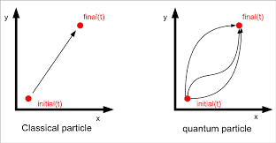
If the operator $(2.36)$ is known on the negative imaginary axis $(t=0, \tau \geq 0)$, one can perform an analytic continuation to the real axis $(t, \tau=0)$. The analytic continuation to complex time $t \rightarrow-\mathrm{i} \tau$ corresponds to a transition from the Minkowski metric $\mathrm{d} s^{2}=d t^{2}-\mathrm{d} x^{2}-\mathrm{d} y^{2}-\mathrm{d} z^{2}$ to a metric with Euclidean signature. Hence a theory with imaginary time is called Euclidean theory.
The time evolution operator $\hat{K}(t)$ exists for real time and defines a oneparametric unitary group. It fulfills the Schrödinger equation
$$
\mathrm{i} \frac{\mathrm{d}}{\mathrm{d} t} \hat{K}(t)=\hat{H} \hat{K}(t)
$$
with a complex and oscillating kernel $K\left(t, q^{\prime}, q\right)=\left\langle q^{\prime}|\hat{K}(t)| q\right\rangle$. For imaginary time we have a Hermitian (and not unitary) evolution operator
$$
\hat{K}(\tau)=\mathrm{e}^{-\tau \hat{H}}
$$
with positive spectrum. The $\hat{K}(\tau)$ exist for positive $\tau$ and form a semi-group only. For almost all initial data, evolution back into the “imaginary past” is impossible.
The evolution operator for imaginary time satisfies the heat equation
$$
\frac{\mathrm{d}}{\mathrm{d} \tau} \hat{K}(\tau)=-\hat{H} \hat{K}(\tau)
$$
instead of the Schrödinger equation and has kernel
$$
K\left(\tau, q^{\prime}, q\right)=\left\langle q^{\prime}\left|\mathrm{e}^{-\tau \hat{H}}\right| q\right\rangle, \quad K\left(0, q^{\prime}, q\right)=\delta\left(q^{\prime}, q\right)
$$
This kernel is real ${ }^{1}$ for a real Hamiltonian. Furthermore it is strictly positive:
物理代写|量子场论代写Quantum field theory代考|Imaginary Time Path Integral
To formulate the path integral for imaginary time, we employ the product formula $(2.28)$, which follows from the product formula (2.27) through the substitution of it by $\tau$. For such systems the analog of $(2.31)$ for Euclidean time $\tau$ is obtained by the substitution of $i \varepsilon$ by $\varepsilon$. Thus we tind
$$
\begin{aligned}
K\left(\tau, q^{\prime}, q\right) &=\left\langle\hat{q}^{\prime}\left|\mathrm{e}^{-\tau \hat{H} / \hbar}\right| \hat{q}\right\rangle \
&=\lim {n \rightarrow \infty} \int \mathrm{d} q{1} \cdots \mathrm{d} q_{n-1}\left(\frac{m}{2 \pi \hbar \varepsilon}\right)^{n / 2} \mathrm{e}^{-S_{\mathrm{E}}\left(q_{0}, q_{1}, \ldots, q_{n}\right) / \hbar} \
S_{\mathrm{E}}(\ldots) &=\varepsilon \sum_{j=0}^{n-1}\left{\frac{m}{2}\left(\frac{q_{j+1}-q_{j}}{\varepsilon}\right)^{2}+V\left(q_{j}\right)\right}
\end{aligned}
$$
where $q_{0}=q$ and $q_{n}=q^{\prime}$. The multidimensional integral represents the sum over all broken-line paths from $q$ to $q^{\prime}$. Interpreting $S_{\mathrm{E}}$ as Hamiltonian of a classical lattice model and $\hbar$ as temperature, it is (up to the fixed endpoints) the partition function of a one-dimensional lattice model on a lattice with $n+1$ sites. The realvalued variable $q_{j}$ defined on site $j$ enters the action $S_{\mathrm{E}}$ which contains interactions between the variables $q_{j}$ and $q_{j+1}$ at neighboring sites. The values of the lattice field
$$
{0,1, \ldots, n-1, n} \rightarrow\left{q_{0}, q_{1}, \ldots, q_{n-1}, q_{n}\right}
$$
are prescribed at the endpoints $q_{0}=q$ and $q_{n}=q^{\prime}$. Note that the classical limit $\hbar \rightarrow 0$ corresponds to the low-temperature limit of the lattice system.
The multidimensional integral (2.52) corresponds to the summation over all path on the time lattice. What happens to the finite-dimensional integral when we take the continuum limit $n \rightarrow \infty$ ? Then we obtain the Euclidean path integral representation for the positive kernel
$$
K\left(\tau, q^{\prime}, q\right)=\left\langle q^{\prime}\left|\mathrm{e}^{-\tau \hat{H} / h}\right| q\right\rangle=C \int_{q(0)=q}^{q(\tau)=q^{\prime}} \mathscr{D} q \mathrm{e}^{-S_{\mathrm{E}}[q] / h}
$$
The integrand contains the Euclidean action
$$
S_{\mathrm{E}}[q]=\int_{0}^{\tau} d \sigma\left{\frac{m}{2} \dot{q}^{2}+V(q(\sigma))\right}
$$
which for many physical systems is bounded from below.
物理代写|量子场论代写Quantum field theory代考|Path Integral in Quantum Statistics
The Euclidean path integral formulation immediately leads to an interesting connection between quantum statistical mechanics and classical statistical physics. Indeed, if we set $\tau / \hbar \equiv \beta$ and integrate over $q=q^{\prime}$ in (2.53), then we end up with the path integral representation for the canonical partition function of a quantum system with Hamiltonian $\hat{H}$ at inverse temperature $\beta=1 / k_{B} T$. More precisely, setting $q=q^{\prime}$ and $\tau=\hbar \beta$ in the left-hand side of this formula, then the integral over $q$ yields the trace of $\exp (-\beta \hat{H})$, which is just the canonical partition function,
$$
\int \mathrm{d} q K(\hbar \beta, q, q)=\operatorname{tr} \mathrm{e}^{-\beta \hat{H}}=Z(\beta)=\sum \mathrm{e}^{-\beta E_{n}} \quad \text { with } \quad \beta=\frac{1}{k_{B} T}
$$
Setting $q=q^{\prime}$ in the Euclidean path integral in (2.53) means that we integrate over paths beginning and ending at $q$ during the imaginary time interval $[0, \hbar \beta]$. The final integral over $q$ leads to the path integral over all periodic paths with period $\hbar \beta$
$$
Z(\beta)=C \oint \mathscr{D} q \mathrm{e}^{-S_{\mathrm{E}}[q] / \hbar}, \quad q(\hbar \beta)=q(0)
$$
For example, the kernell of the harmonic oscillator in $(2.43)$ on the diagonal is
$$
K_{\omega}(\beta, q, q)=\sqrt{\frac{m \omega}{2 \pi \sinh (\omega \beta)}} \exp \left{-m \omega \tanh (\omega \beta / 2) q^{2}\right}
$$
where we used units with $\hbar=1$. The integral over $q$ yields the partition function
$$
\begin{aligned}
Z(\beta) &=\sqrt{\frac{m \omega}{2 \pi \sinh (\omega \beta)}} \int \mathrm{d} q \exp \left{-m \omega \tanh (\omega \beta / 2) q^{2}\right} \
&=\frac{1}{2 \sinh (\omega \beta / 2)}=\frac{\mathrm{e}^{-\omega \beta / 2}}{1-\mathrm{e}^{-\omega \beta}}=\mathrm{e}^{-\omega \beta / 2} \sum_{n=0}^{\infty} \mathrm{e}^{-n \omega \beta}
\end{aligned}
$$
where we used $\sinh x=2 \sinh x / 2 \cosh x / 2$. A comparison with the spectral sum over all energies in (2.55) yields the energies of the oscillator with (angular) frequency $\omega$,
$$
E_{n}=\omega\left(n+\frac{1}{2}\right), \quad n=0,1,2, \ldots
$$
For large values of $\omega \beta$, i.e., for very low temperature, the spectral sum is dominated by the contribution of the ground state energy. Thus for cold systems, the free energy converges to the ground state energy
$$
F(\beta) \equiv-\frac{1}{\beta} \log Z(\beta) \stackrel{\omega \beta \rightarrow \infty}{\longrightarrow} E_{0}
$$
One often is interested in the energies and wave functions of excited states. We now discuss an elegant method to extract this information from the path integral.
量子场论代考
物理代写|量子场论代写Quantum field theory代考|Quantum Mechanics in Imaginary Time
酉时间演化算子具有谱表示
ķ^(吨)=和−一世H^吨=∫和−一世和吨 d磷^和,在哪里磷^和是哈密顿量的谱族。如果H^有离散谱,则磷^和是在子空间上的正交投影H由能量小于的所有特征函数跨越和. 在下文中,我们假设哈密顿算子是从下面有界的。然后我们可以减去它的基态能量得到一个非负的H^(2.35) 中的积分限制为 0 并且∞. 随着替换吨→吨−一世τ, 我们获得
和−(τ+一世吨)H^=∫0∞和−和(τ+一世吨)d磷^和
这在下复半平面中定义了一个全纯半群
和=吨−一世τ∈C,τ≥0
如果运营商(2.36)在负虚轴上已知(吨=0,τ≥0), 可以对实轴进行解析延拓(吨,τ=0). 复杂时间的解析延展吨→−一世τ对应于 Minkowski 度量的转换ds2=d吨2−dX2−d是2−d和2到具有欧几里得签名的度量。因此,具有虚时间的理论称为欧几里得理论。
时间演化算子ķ^(吨)实时存在并定义一个参数酉群。它满足薛定谔方程
一世dd吨ķ^(吨)=H^ķ^(吨)
具有复杂和振荡的内核ķ(吨,q′,q)=⟨q′|ķ^(吨)|q⟩. 对于虚构的时间,我们有一个 Hermitian(而不是单一的)进化算子
ķ^(τ)=和−τH^
具有正谱。这ķ^(τ)为积极而存在τ并且只形成一个半群。对于几乎所有的初始数据,进化回“想象的过去”是不可能的。
虚时间演化算子满足热方程
ddτķ^(τ)=−H^ķ^(τ)
而不是薛定谔方程并且有核
ķ(τ,q′,q)=⟨q′|和−τH^|q⟩,ķ(0,q′,q)=d(q′,q)
这个内核是真的1对于一个真正的哈密顿量。此外,它是严格肯定的:
物理代写|量子场论代写Quantum field theory代考|Imaginary Time Path Integral
为了制定虚时间的路径积分,我们使用乘积公式(2.28), 通过将乘积公式 (2.27) 替换为τ. 对于这样的系统,模拟(2.31)欧几里得时间τ通过替换获得一世e经过e. 因此我们认为
\begin{aligned} 左(\tau, q^{\prime}, q\right) &=\left\langle\hat{q}^{\prime}\left|\mathrm{e}^{- \tau \hat{H} / \hbar}\right| \hat{q}\right\rangle\&=\lim{n\rightarrow\infty}\int \mathrm{d}q{1}\cdots\mathrm{d}q_{n-1}\left(\frac {m}{2 \pi \hbar \value psilon}\right)^{n/2}\mathrm{e}^{-S_{\mathrm{E}}\left(q_{0}, q_{1} , \ldots, q_{n}\right) / \hbar}\S_{\mathrm{E}}(\ldots) &=\varepsilon \sum_{j=0}^{n-1}\left{\frac { m}{2}\left(\frac{q_{j+1}-q_{j}}{\valuepsilon}\right)^{2}+V\left(q_{j}\right)\right} \结束{对齐}\begin{aligned} 左(\tau, q^{\prime}, q\right) &=\left\langle\hat{q}^{\prime}\left|\mathrm{e}^{- \tau \hat{H} / \hbar}\right| \hat{q}\right\rangle\&=\lim{n\rightarrow\infty}\int \mathrm{d}q{1}\cdots\mathrm{d}q_{n-1}\left(\frac {m}{2 \pi \hbar \value psilon}\right)^{n/2}\mathrm{e}^{-S_{\mathrm{E}}\left(q_{0}, q_{1} , \ldots, q_{n}\right) / \hbar}\S_{\mathrm{E}}(\ldots) &=\varepsilon \sum_{j=0}^{n-1}\left{\frac { m}{2}\left(\frac{q_{j+1}-q_{j}}{\valuepsilon}\right)^{2}+V\left(q_{j}\right)\right} \结束{对齐}
在哪里q0=q和qn=q′. 多维积分表示所有虚线路径的总和q至q′. 口译小号和作为经典晶格模型的哈密顿量和ℏ作为温度,它是(直到固定端点)晶格上的一维晶格模型的配分函数n+1网站。实值变量qj现场定义j进入动作小号和其中包含变量之间的相互作用qj和qj+1在邻近站点。格域的值
{0,1, \ldots, n-1, n} \rightarrow\left{q_{0}, q_{1}, \ldots, q_{n-1}, q_{n}\right}{0,1, \ldots, n-1, n} \rightarrow\left{q_{0}, q_{1}, \ldots, q_{n-1}, q_{n}\right}
在端点规定q0=q和qn=q′. 注意经典极限ℏ→0对应于晶格系统的低温极限。
多维积分 (2.52) 对应于时间格上所有路径的总和。当我们取连续极限时,有限维积分会发生什么n→∞? 然后我们得到正核的欧几里得路径积分表示
ķ(τ,q′,q)=⟨q′|和−τH^/H|q⟩=C∫q(0)=qq(τ)=q′Dq和−小号和[q]/H
被积函数包含欧几里得动作
S_{\mathrm{E}}[q]=\int_{0}^{\tau} d \sigma\left{\frac{m}{2} \dot{q}^{2}+V(q( \sigma))\对}S_{\mathrm{E}}[q]=\int_{0}^{\tau} d \sigma\left{\frac{m}{2} \dot{q}^{2}+V(q( \sigma))\对}
对于许多物理系统来说,它是从下面限定的。
物理代写|量子场论代写Quantum field theory代考|Path Integral in Quantum Statistics
欧几里得路径积分公式立即导致了量子统计力学和经典统计物理学之间的有趣联系。确实,如果我们设置τ/ℏ≡b并整合过来q=q′在 (2.53) 中,我们最终得到具有哈密顿量的量子系统的规范配分函数的路径积分表示H^在逆温b=1/ķ乙吨. 更准确地说,设置q=q′和τ=ℏb在这个公式的左边,那么积分超过q产生的痕迹经验(−bH^),这只是典型的分区函数,
∫dqķ(ℏb,q,q)=tr和−bH^=从(b)=∑和−b和n 和 b=1ķ乙吨
环境q=q′在(2.53)中的欧几里得路径积分中意味着我们在开始和结束于的路径上积分q在虚构的时间间隔内[0,ℏb]. 最后的积分超过q导致所有周期路径上的路径积分ℏb
从(b)=C∮Dq和−小号和[q]/ℏ,q(ℏb)=q(0)
例如,谐振子的 kernell(2.43)对角线上是
K_{\omega}(\beta, q, q)=\sqrt{\frac{m \omega}{2 \pi \sinh (\omega \beta)}} \exp \left{-m \omega \tanh ( \omega \beta / 2) q^{2}\right}K_{\omega}(\beta, q, q)=\sqrt{\frac{m \omega}{2 \pi \sinh (\omega \beta)}} \exp \left{-m \omega \tanh ( \omega \beta / 2) q^{2}\right}
我们在哪里使用单位ℏ=1. 积分超过q产生配分函数
\begin{对齐}Z(\beta)&=\sqrt{\frac{m\omega}{2\pi\sinh(\omega\beta)}}\int\mathrm{d}q\exp\left{- m\omega\tanh(\omega\beta/2)q^{2}\right}\&=\frac{1}2\sinh(\omega\beta/2)}=\mathrm{e}^{- \omega\beta/2}{1-\mathrm{e}^{-\omega\beta}}=\mathrm{e}^{-\omega\beta/2}\sum_{n=0}^{\ infty} \ mathrm {e} ^ {- n \ omega \ beta} \ end {对齐}\begin{对齐}Z(\beta)&=\sqrt{\frac{m\omega}{2\pi\sinh(\omega\beta)}}\int\mathrm{d}q\exp\left{- m\omega\tanh(\omega\beta/2)q^{2}\right}\&=\frac{1}2\sinh(\omega\beta/2)}=\mathrm{e}^{- \omega\beta/2}{1-\mathrm{e}^{-\omega\beta}}=\mathrm{e}^{-\omega\beta/2}\sum_{n=0}^{\ infty} \ mathrm {e} ^ {- n \ omega \ beta} \ end {对齐}
我们用过的地方出生X=2出生X/2科什X/2. 与 (2.55) 中所有能量的频谱总和进行比较,得出具有(角)频率的振荡器的能量ω,
和n=ω(n+12),n=0,1,2,…
对于较大的值ωb,即对于非常低的温度,谱和主要由基态能量的贡献决定。因此对于冷系统,自由能收敛到基态能量
F(b)≡−1b日志从(b)⟶ωb→∞和0
人们经常对激发态的能量和波函数感兴趣。我们现在讨论一种从路径积分中提取此信息的优雅方法。

统计代写请认准statistics-lab™. statistics-lab™为您的留学生涯保驾护航。
金融工程代写
金融工程是使用数学技术来解决金融问题。金融工程使用计算机科学、统计学、经济学和应用数学领域的工具和知识来解决当前的金融问题,以及设计新的和创新的金融产品。
非参数统计代写
非参数统计指的是一种统计方法,其中不假设数据来自于由少数参数决定的规定模型;这种模型的例子包括正态分布模型和线性回归模型。
广义线性模型代考
广义线性模型(GLM)归属统计学领域,是一种应用灵活的线性回归模型。该模型允许因变量的偏差分布有除了正态分布之外的其它分布。
术语 广义线性模型(GLM)通常是指给定连续和/或分类预测因素的连续响应变量的常规线性回归模型。它包括多元线性回归,以及方差分析和方差分析(仅含固定效应)。
有限元方法代写
有限元方法(FEM)是一种流行的方法,用于数值解决工程和数学建模中出现的微分方程。典型的问题领域包括结构分析、传热、流体流动、质量运输和电磁势等传统领域。
有限元是一种通用的数值方法,用于解决两个或三个空间变量的偏微分方程(即一些边界值问题)。为了解决一个问题,有限元将一个大系统细分为更小、更简单的部分,称为有限元。这是通过在空间维度上的特定空间离散化来实现的,它是通过构建对象的网格来实现的:用于求解的数值域,它有有限数量的点。边界值问题的有限元方法表述最终导致一个代数方程组。该方法在域上对未知函数进行逼近。[1] 然后将模拟这些有限元的简单方程组合成一个更大的方程系统,以模拟整个问题。然后,有限元通过变化微积分使相关的误差函数最小化来逼近一个解决方案。
tatistics-lab作为专业的留学生服务机构,多年来已为美国、英国、加拿大、澳洲等留学热门地的学生提供专业的学术服务,包括但不限于Essay代写,Assignment代写,Dissertation代写,Report代写,小组作业代写,Proposal代写,Paper代写,Presentation代写,计算机作业代写,论文修改和润色,网课代做,exam代考等等。写作范围涵盖高中,本科,研究生等海外留学全阶段,辐射金融,经济学,会计学,审计学,管理学等全球99%专业科目。写作团队既有专业英语母语作者,也有海外名校硕博留学生,每位写作老师都拥有过硬的语言能力,专业的学科背景和学术写作经验。我们承诺100%原创,100%专业,100%准时,100%满意。
随机分析代写
随机微积分是数学的一个分支,对随机过程进行操作。它允许为随机过程的积分定义一个关于随机过程的一致的积分理论。这个领域是由日本数学家伊藤清在第二次世界大战期间创建并开始的。
时间序列分析代写
随机过程,是依赖于参数的一组随机变量的全体,参数通常是时间。 随机变量是随机现象的数量表现,其时间序列是一组按照时间发生先后顺序进行排列的数据点序列。通常一组时间序列的时间间隔为一恒定值(如1秒,5分钟,12小时,7天,1年),因此时间序列可以作为离散时间数据进行分析处理。研究时间序列数据的意义在于现实中,往往需要研究某个事物其随时间发展变化的规律。这就需要通过研究该事物过去发展的历史记录,以得到其自身发展的规律。
回归分析代写
多元回归分析渐进(Multiple Regression Analysis Asymptotics)属于计量经济学领域,主要是一种数学上的统计分析方法,可以分析复杂情况下各影响因素的数学关系,在自然科学、社会和经济学等多个领域内应用广泛。
MATLAB代写
MATLAB 是一种用于技术计算的高性能语言。它将计算、可视化和编程集成在一个易于使用的环境中,其中问题和解决方案以熟悉的数学符号表示。典型用途包括:数学和计算算法开发建模、仿真和原型制作数据分析、探索和可视化科学和工程图形应用程序开发,包括图形用户界面构建MATLAB 是一个交互式系统,其基本数据元素是一个不需要维度的数组。这使您可以解决许多技术计算问题,尤其是那些具有矩阵和向量公式的问题,而只需用 C 或 Fortran 等标量非交互式语言编写程序所需的时间的一小部分。MATLAB 名称代表矩阵实验室。MATLAB 最初的编写目的是提供对由 LINPACK 和 EISPACK 项目开发的矩阵软件的轻松访问,这两个项目共同代表了矩阵计算软件的最新技术。MATLAB 经过多年的发展,得到了许多用户的投入。在大学环境中,它是数学、工程和科学入门和高级课程的标准教学工具。在工业领域,MATLAB 是高效研究、开发和分析的首选工具。MATLAB 具有一系列称为工具箱的特定于应用程序的解决方案。对于大多数 MATLAB 用户来说非常重要,工具箱允许您学习和应用专业技术。工具箱是 MATLAB 函数(M 文件)的综合集合,可扩展 MATLAB 环境以解决特定类别的问题。可用工具箱的领域包括信号处理、控制系统、神经网络、模糊逻辑、小波、仿真等。