如果你也在 怎样代写多元统计分析Multivariate Statistical Analysis这个学科遇到相关的难题，请随时右上角联系我们的24/7代写客服。

多变量统计分析Multivariate Statistical Analysis关注的是由一些个体或物体的测量数据集组成的数据。样本数据可能是从某个城市的学童群体中随机抽取的一些个体的身高和体重，或者对一组测量数据进行统计处理，例如从两个物种中抽取的鸢尾花花瓣的长度和宽度以及萼片的长度和宽度，或者我们可以研究对一些学生进行的智力测试的分数。
在一个特定的个体上，有p=#$的测量集合。
$n=#$ 观察值 $=$ 样本大小

statistics-lab™ 为您的留学生涯保驾护航 在代写多元统计分析Multivariate Statistical Analysis方面已经树立了自己的口碑, 保证靠谱, 高质且原创的统计Statistics代写服务。我们的专家在代写多元统计分析Multivariate Statistical Analysis代写方面经验极为丰富，各种代写多元统计分析Multivariate Statistical Analysis相关的作业也就用不着 说。

我们提供的多元统计分析Multivariate Statistical Analysis及其相关学科的代写，服务范围广, 其中包括但不限于:

• Statistical Inference 统计推断
• Statistical Computing 统计计算
• Advanced Probability Theory 高等楖率论
• Advanced Mathematical Statistics 高等数理统计学
• (Generalized) Linear Models 广义线性模型
• Statistical Machine Learning 统计机器学习
• Longitudinal Data Analysis 纵向数据 分析
• Foundations of Data Science 数据科学基础

统计代写|多元统计分析作业代写Multivariate Statistical Analysis代考|Transformations, assessing normality and independence

In Section $3.4$ we discussed the use of transformations to create new variables. In this chapter we discuss transforming the data to obtain a distribution that is approximately normal. This is of particular interest for exploratory data analysis. For confirmatory data analysis (as described in Chapter 1) one should choose any appropriate transformations of variables prior to performing any analyses. Section $5.2$ shows how transformations change the shape of distributions. Section $5.3$ discusses several methods for deciding when a transformation should be made and how to find a suitable transformation. An iterative scheme is proposed that helps to zero in on a good transformation and statistical tests for normality are evaluated. Section $5.4$ presents simple graphical methods for determining if the data are independent. Section $5.5$ provides an overview of the methods used in the four statistical software packages for topics discussed in this chapter. In this chapter, we rely heavily on graphical methods: see Cook and Weisberg (1994) and Tufte (2001).

Each computer software package offers the users information to help decide if their data are normally distributed. The packages provide convenient methods for transforming the data to achieve approximate normality. They also include some output for checking the independence of the observations. Hence the assumption of independent, normally distributed data that is made in many statistical tests can be assessed, at least approximately. Note that it has been shown that inference can be robust in many research settings even with highly non-normal data (see Lumley et al., 2002). Additionally, many investigators may try to discard the most obvious outliers prior to assessing normality because such outliers can grossly distort the distribution, but discarding outliers is generally not advised unless it is concluded that an error has occurred in the measurement, recording or entry of these observations. Some researchers also consider removing inconsistent or extreme observations (see Osborne and Overbay, 2004), but such a decision depends heavily on the circumstances surrounding the research topic and should always be documented.

统计代写|多元统计分析作业代写Multivariate Statistical Analysis代考|Common transformations

For exploratory analysis of data it may be useful to transform certain variables before performing the analyses. Examples are found in the next section and in Chapter 7. In this section we present some common transformations. If you are familiar with this subject, you may wish to skip to the next section.

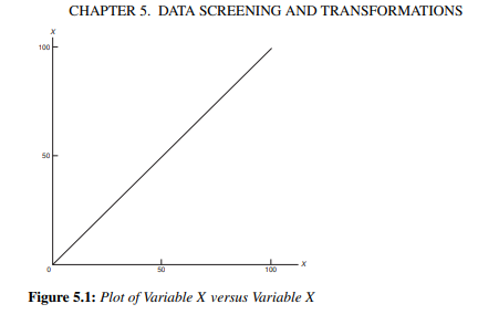
To develop a feel for transformations, let us examine a plot of transformed values versus the original values of the variable. To begin with, a plot of values of a variable $X$ against itself produces a $45^{\circ}$ diagonal line going through the origin, as shown in Figure 5.1.

One of the most commonly performed transformations is taking the logarithm (log) to base 10 . Recall that the logarithm is the number that satisfies the relationship $X=10^{Y}$. That is, the logarithm of $X$ is the power $Y$ to which 10 must be raised in order to produce $X$. As shown in Figure $5.2$ in plot a, the logarithm of 10 is 1 since $10=10^{1}$. Similarly, the logarithm of 1 is 0 since $1=10^{\circ}$, and the logarithm of 100 is 2 since $100=10^{2}$. Other values of logarithms can be obtained from tables of common logarithms, from a hand calculator with a log function, or from statistical packages by using the transformation options. All statistical packages discussed in this book allow the user to make this transformation as well as others.

统计代写|多元统计分析作业代写Multivariate Statistical Analysis代考|Selecting appropriate transformations

In the theoretical development of statistical methods some assumptions might be made regarding the distribution of the variables being analyzed. The most commonly assumed distribution for continuous observations is the normal, or Gaussian, distribution. Nevertheless, even if the values of a variable are not or are far from being normally distributed, the averages of such data can be shown to be normally distributed for large enough sample sizes. This is a pivotal mathematical result called the Central Limit Theorem. For a review and discussion of what sample size can be considered “large enough” in relation to highly non-normal data see Lumley et al. (2002). In this section, methods for assessing normality and for choosing a transformation to induce normality are presented.
Assessing normality using histograms
The left graph of Figure 5.4a illustrates the appearance of an ideal histogram, or density function, of normally distributed data. The values of the variable $X$ are plotted on the horizontal axis. The range of $X$ is partitioned into numerous intervals of equal length and the proportion of observations in each interval is plotted on the vertical axis (see also Section 4.2). The mean is in the center of the distribution and is equal to zero in this hypothetical histogram. The distribution is symmetric about the mean; that is, intervals equidistant from the mean have equal proportions of observations (or the same height in the histogram). If you place a mirror vertically at the mean of a symmetric histogram, the right side should be a mirror image of the left side. A distribution may be symmetric and still.

假设检验代写

统计代写|多元统计分析作业代写Multivariate Statistical Analysis代考|Transformations, assessing normality and independence

在部分3.4我们讨论了使用转换来创建新变量。在本章中，我们讨论如何转换数据以获得近似正态分布。这对于探索性数据分析特别感兴趣。对于验证性数据分析（如第 1 章所述），应在执行任何分析之前选择任何适当的变量转换。部分5.2显示变换如何改变分布的形状。部分5.3讨论了决定何时进行转换以及如何找到合适的转换的几种方法。提出了一种迭代方案，有助于将良好的转换归零，并评估正态性的统计测试。部分5.4提供了用于确定数据是否独立的简单图形方法。部分5.5概述了本章讨论的主题的四个统计软件包中使用的方法。在本章中，我们严重依赖图形方法：参见 Cook 和 Weisberg (1994) 和 Tufte (2001)。

每个计算机软件包都为用户提供信息，以帮助确定他们的数据是否正常分布。这些包提供了转换数据以实现近似正态性的便捷方法。它们还包括一些用于检查观察独立性的输出。因此，可以至少近似地评估在许多统计测试中做出的独立、正态分布数据的假设。请注意，已经表明，即使使用高度非正态的数据，推理在许多研究环境中也是稳健的（参见 Lumley 等人，2002 年）。此外，许多调查人员可能会在评估正态性之前尝试丢弃最明显的异常值，因为这些异常值会严重扭曲分布，但通常不建议丢弃异常值，除非得出结论认为在这些观察结果的测量、记录或输入中发生了错误。一些研究人员还考虑删除不一致或极端的观察结果（参见 Osborne 和 Overbay，2004 年），但这样的决定很大程度上取决于围绕研究主题的情况，并且应始终记录在案。

统计代写|多元统计分析作业代写Multivariate Statistical Analysis代考|Common transformations

对于数据的探索性分析，在执行分析之前转换某些变量可能很有用。示例在下一节和第 7 章中找到。在本节中，我们将介绍一些常见的转换。如果您熟悉此主题，您可能希望跳到下一部分。

为了培养对转换的感觉，让我们检查转换值与变量原始值的关系图。首先，一个变量的值图X对自己产生一个45∘对角线穿过原点，如图 5.1 所示。

最常执行的转换之一是将对数 (log) 以 10 为底。回想一下，对数是满足关系的数X=10和. 也就是说，对数X是权力和必须提高到 10 才能生产X. 如图5.2在图 a 中，10 的对数为 1，因为10=101. 同样，1 的对数为 0，因为1=10∘, 100 的对数是 2100=102. 其他对数值可以从常用对数表、具有对数功能的手动计算器或使用转换选项从统计包中获得。本书中讨论的所有统计软件包都允许用户进行这种转换以及其他转换。

统计代写|多元统计分析作业代写Multivariate Statistical Analysis代考|Selecting appropriate transformations

在统计方法的理论发展中，可能会对所分析的变量的分布做出一些假设。连续观测最常见的假设分布是正态分布或高斯分布。然而，即使变量的值不是正态分布或远非正态分布，对于足够大的样本量，这些数据的平均值也可以显示为正态分布。这是一个关键的数学结果，称为中心极限定理。有关与高度非正态数据相关的样本量可以被视为“足够大”的审查和讨论，请参见 Lumley 等人。（2002 年）。在本节中，介绍了评估正态性和选择转换以诱导正态性的方法。
使用直方图评估正态性
图 5.4a 的左图说明了正态分布数据的理想直方图或密度函数的外观。变量的值X绘制在水平轴上。的范围X被划分为许多等长的区间，并且每个区间中的观察比例绘制在垂直轴上（另见第 4.2 节）。均值位于分布的中心，在此假设直方图中为零。分布关于均值对称；也就是说，与平均值等距的区间具有相同比例的观测值（或直方图中的相同高度）。如果在对称直方图的平均值上垂直放置镜子，则右侧应该是左侧的镜像。分布可能是对称且静止的。

统计代写请认准statistics-lab™. statistics-lab™为您的留学生涯保驾护航。

随机过程代考

在概率论概念中，随机过程是随机变量的集合。 若一随机系统的样本点是随机函数，则称此函数为样本函数，这一随机系统全部样本函数的集合是一个随机过程。 实际应用中，样本函数的一般定义在时间域或者空间域。 随机过程的实例如股票和汇率的波动、语音信号、视频信号、体温的变化，随机运动如布朗运动、随机徘徊等等。

贝叶斯方法代考

贝叶斯统计概念及数据分析表示使用概率陈述回答有关未知参数的研究问题以及统计范式。后验分布包括关于参数的先验分布，和基于观测数据提供关于参数的信息似然模型。根据选择的先验分布和似然模型，后验分布可以解析或近似，例如，马尔科夫链蒙特卡罗 (MCMC) 方法之一。贝叶斯统计概念及数据分析使用后验分布来形成模型参数的各种摘要，包括点估计，如后验平均值、中位数、百分位数和称为可信区间的区间估计。此外，所有关于模型参数的统计检验都可以表示为基于估计后验分布的概率报表。

广义线性模型代考

广义线性模型（GLM）归属统计学领域，是一种应用灵活的线性回归模型。该模型允许因变量的偏差分布有除了正态分布之外的其它分布。

statistics-lab作为专业的留学生服务机构，多年来已为美国、英国、加拿大、澳洲等留学热门地的学生提供专业的学术服务，包括但不限于Essay代写，Assignment代写，Dissertation代写，Report代写，小组作业代写，Proposal代写，Paper代写，Presentation代写，计算机作业代写，论文修改和润色，网课代做，exam代考等等。写作范围涵盖高中，本科，研究生等海外留学全阶段，辐射金融，经济学，会计学，审计学，管理学等全球99%专业科目。写作团队既有专业英语母语作者，也有海外名校硕博留学生，每位写作老师都拥有过硬的语言能力，专业的学科背景和学术写作经验。我们承诺100%原创，100%专业，100%准时，100%满意。

机器学习代写

随着AI的大潮到来，Machine Learning逐渐成为一个新的学习热点。同时与传统CS相比，Machine Learning在其他领域也有着广泛的应用，因此这门学科成为不仅折磨CS专业同学的“小恶魔”，也是折磨生物、化学、统计等其他学科留学生的“大魔王”。学习Machine learning的一大绊脚石在于使用语言众多，跨学科范围广，所以学习起来尤其困难。但是不管你在学习Machine Learning时遇到任何难题，StudyGate专业导师团队都能为你轻松解决。

多元统计分析代考

基础数据: $N$ 个样本， $P$ 个变量数的单样本，组成的横列的数据表
变量定性: 分类和顺序；变量定量：数值
数学公式的角度分为: 因变量与自变量

时间序列分析代写

随机过程，是依赖于参数的一组随机变量的全体，参数通常是时间。 随机变量是随机现象的数量表现，其时间序列是一组按照时间发生先后顺序进行排列的数据点序列。通常一组时间序列的时间间隔为一恒定值（如1秒，5分钟，12小时，7天，1年），因此时间序列可以作为离散时间数据进行分析处理。研究时间序列数据的意义在于现实中，往往需要研究某个事物其随时间发展变化的规律。这就需要通过研究该事物过去发展的历史记录，以得到其自身发展的规律。

回归分析代写

多元回归分析渐进（Multiple Regression Analysis Asymptotics）属于计量经济学领域，主要是一种数学上的统计分析方法，可以分析复杂情况下各影响因素的数学关系，在自然科学、社会和经济学等多个领域内应用广泛。

MATLAB代写

MATLAB 是一种用于技术计算的高性能语言。它将计算、可视化和编程集成在一个易于使用的环境中，其中问题和解决方案以熟悉的数学符号表示。典型用途包括：数学和计算算法开发建模、仿真和原型制作数据分析、探索和可视化科学和工程图形应用程序开发，包括图形用户界面构建MATLAB 是一个交互式系统，其基本数据元素是一个不需要维度的数组。这使您可以解决许多技术计算问题，尤其是那些具有矩阵和向量公式的问题，而只需用 C 或 Fortran 等标量非交互式语言编写程序所需的时间的一小部分。MATLAB 名称代表矩阵实验室。MATLAB 最初的编写目的是提供对由 LINPACK 和 EISPACK 项目开发的矩阵软件的轻松访问，这两个项目共同代表了矩阵计算软件的最新技术。MATLAB 经过多年的发展，得到了许多用户的投入。在大学环境中，它是数学、工程和科学入门和高级课程的标准教学工具。在工业领域，MATLAB 是高效研究、开发和分析的首选工具。MATLAB 具有一系列称为工具箱的特定于应用程序的解决方案。对于大多数 MATLAB 用户来说非常重要，工具箱允许您学习和应用专业技术。工具箱是 MATLAB 函数（M 文件）的综合集合，可扩展 MATLAB 环境以解决特定类别的问题。可用工具箱的领域包括信号处理、控制系统、神经网络、模糊逻辑、小波、仿真等。