如果你也在 怎样代写多元统计分析Multivariate Statistical Analysis这个学科遇到相关的难题,请随时右上角联系我们的24/7代写客服。
多变量统计分析Multivariate Statistical Analysis关注的是由一些个体或物体的测量数据集组成的数据。样本数据可能是从某个城市的学童群体中随机抽取的一些个体的身高和体重,或者对一组测量数据进行统计处理,例如从两个物种中抽取的鸢尾花花瓣的长度和宽度以及萼片的长度和宽度,或者我们可以研究对一些学生进行的智力测试的分数。
在一个特定的个体上,有p=#$的测量集合。
$n=#$ 观察值 $=$ 样本大小
statistics-lab™ 为您的留学生涯保驾护航 在代写多元统计分析Multivariate Statistical Analysis方面已经树立了自己的口碑, 保证靠谱, 高质且原创的统计Statistics代写服务。我们的专家在代写多元统计分析Multivariate Statistical Analysis代写方面经验极为丰富,各种代写多元统计分析Multivariate Statistical Analysis相关的作业也就用不着 说。
我们提供的多元统计分析Multivariate Statistical Analysis及其相关学科的代写,服务范围广, 其中包括但不限于:
- Statistical Inference 统计推断
- Statistical Computing 统计计算
- Advanced Probability Theory 高等楖率论
- Advanced Mathematical Statistics 高等数理统计学
- (Generalized) Linear Models 广义线性模型
- Statistical Machine Learning 统计机器学习
- Longitudinal Data Analysis 纵向数据 分析
- Foundations of Data Science 数据科学基础
统计代写|多元统计分析作业代写Multivariate Statistical Analysis代考|Criteria for variable selection
Residual Sum of Squares
As discussed in Chapter 8, the least squares method of estimation minimizes the residual sum of squares about the regression plane $\left.\left[\mathrm{RSS}=\Sigma(Y-\hat{Y})^{2}\right)\right]$. Therefore an implicit criterion is the value of RSS. In deciding between alternative subsets of variables, the investigator would select the one producing the smaller RSS if this criterion were used in a mechanical fashion. Note, however, that
$$
\mathrm{RSS}=\sum(Y-\bar{Y})^{2}\left(1-R^{2}\right)
$$
150
CHAPTER 9. VARIABLE SELECTION IN REGRESSION
where $R$ is the multiple correlation coefficient. Therefore minimizing RSS is equivalent to maximizing the multiple correlation coefficient. If just the criterion of maximizing $R$ were used, the investigator would always select all of the independent variables, because the value of $R$ will never decrease by including additional variables.
Adjusted $R^{2}$
Since the multiple correlation coefficient, on the average, overestimates the population correlation coefficient, the investigator may be misled into including too many variables. For example, if the population multiple correlation coefficient is, in fact, equal to zero, the average of all possible values of $R^{2}$ from samples of size $N$ from a multivariate normal population is $P /(N-1)$, where $P$ is the number of independent variables (Wishart et al., 1931). An estimated multiple correlation coefficient that reduces the bias is the adjusted multiple correlation coefficient, denoted by $\bar{R}$. It is related to $R$ by the following equation:
$$
\bar{R}^{2}=R^{2}-\frac{P\left(1-R^{2}\right)}{N-P-1}
$$
统计代写|多元统计分析作业代写Multivariate Statistical Analysis代考|A general $F$ test
Suppose we are convinced that the variables $X_{1}, X_{2}, \ldots, X_{p}$ should be used in the regression equation. Suppose also that measurements on $Q$ additional variables $X_{P+1}, X_{P+2}, \ldots, X_{P+Q}$ are available. Before deciding whether any of the additional variables should be included, we can test the hypothesis that, as a group, the $Q$ variables do not improve the regression equation.
If the regression equation in the population has the form
$$
\begin{gathered}
Y=\alpha+\beta_{1} X_{1}+\beta_{2} X_{2}+\cdots+\beta_{P} X_{P}+\beta_{P+1} X_{P+1} \
+\cdots+\beta_{P+Q} X_{P+Q}+e
\end{gathered}
$$
we test the hypothesis $H_{0}: \beta_{P+1}=\beta_{P+2}=\cdots=\beta_{P+Q}=0$. To perform the test, we first obtain an equation that includes all the $P+Q$ variables, and we obtain the residual sum of squares $\left(\mathrm{RSS}{P+Q}\right)$. Similarly, we obtain an equation that includes only the first $P$ variables and the corresponding residual sum of squares $\left(\operatorname{RSS}{p}\right)$. Then the test statistic is computed as
$$
F=\frac{\left(\operatorname{RSS}{P}-\operatorname{RSS}{P+Q}\right) / Q}{\operatorname{RSS}_{P+Q} /(N-P-Q-1)}
$$
The numerator measures the improvement in the equation from using the additional $Q$ variables. This quantity is never negative. The hypothesis is rejected if the computed $F$ exceeds the tabled $F(1-\alpha)$ with $Q$ and $N-P-Q-1$ degrees of freedom.
This very general test is sometimes referred to as the generalized linear hypothesis test. Essentially, this same test was used in Section $8.9$ to test whether or not it is necessary to report the regression analyses by subgroups. The quantities $P$ and $Q$ can take on any integer values greater than or equal to one. For example, suppose that six variables are available. If we take $P$ equal to 5 and $Q$ equal to 1 , then we are testing $H_{0}: \beta_{6}=0$ in the equation $Y=\alpha+\beta_{1} X_{1}+\beta_{2} X_{2}+\beta_{3} X_{3}+$ $\beta_{4} X_{4}+\beta_{5} X_{5}+\beta_{6} X_{6}+e$. This test is the same as the test that was discussed in Section $8.6$ for the significance of a single regression coefficient.
As another example, in the chemical companies’ data it was already observed that D/E is the best single predictor of the $\mathrm{P} / \mathrm{E}$ ratio. A relevant hypothesis is whether the remaining five variables improve the prediction obtained by D/E alone. Two regressions were run (one with all six variables and one with just D/E), and the results were as follows:
$$
\begin{array}{r}
\mathrm{RSS}{6}=103.06 \ \mathrm{RSS}{1}=176.08 \
P=1, Q=5
\end{array}
$$
统计代写|多元统计分析作业代写Multivariate Statistical Analysis代考|Stepwise regression
The best combination of two variables is NPM1 and PAYOUTR1, with a multiple $R^{2}$ of $0.408$. This combination does not include D/E, as would be the case in stepwise regression (Table 9.3). In stepwise regression the two variables selected were D/E and PAYOUTR1 with a multiple $R^{2}$ of $0.290$. Here stepwise regression does not come close to selecting the best combination of two variables. Here stepwise regression resulted in the fourth-best choice. The third-best combination of two variables is essentially as good as the second best. The best combination of two variables, NPM1 and PAYOUTR1, as chosen by SAS REG, is interesting in light of our earlier interpretation of the variables in Section 9.3. Variable NPM1 measures the efficiency of the operation in converting sales to earnings, while PAYOUTR1 measures the intention to plow earnings back into the company or distribute them to stockholders. These are quite different aspects of current company behavior. In contrast, the debt-to-equity ratio D/E may be, in large part, a historical carry-over from past operations or a reflection of management style.
For the best combination of three variables the value of the multiple $R^{2}$ is $0.482$, only slightly better than the stepwise choice. If $\mathrm{D} / \mathrm{E}$ is a lot simpler to obtain than SALESGR5, the stepwise selection might be preferred since the loss in the multiple $R^{2}$ is negligible. Here the investigator, when given the option of different subsets, might prefer the first (NPM1, PAYOUTR1, SALESGR5) on theoretical grounds, since it is the only option that explicitly includes a measure of growth (SALESGR5). (You should also examine the four-variable combinations in light of the above discussion.)
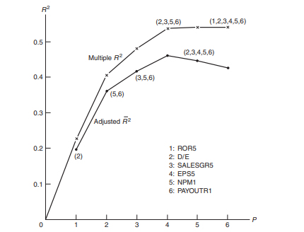
Summarizing the results in the form of Table $9.6$ is advisable. Then plotting the best combination of one, two, three, four, five, or six variables helps the investigator decide how many variables to use. For example, Figure $9.1$ shows a plot of the multiple $R^{2}$ and the adjusted $\bar{R}^{2}$ versus the number of variables included in the best combination in the data set. Note that $R^{2}$ is a nondecreasing function. However, it levels off after four variables. The adjusted $\bar{R}^{2}$ reaches its maximum with four variables (D/E, NPM1, PAYOUTR1, and SALESGR5) and decreases with five and six variables.
Figure $9.2$ shows $C_{p}$ versus $P$ (the number of variables) for the best combinations for the chemical companies’ data. The same combination of four variables selected by the $R^{2}$ criterion minimizes $C_{p}$. A similar graph in Figure $9.3$ shows that AIC is also minimized by the same choice of four variables.
假设检验代写
统计代写|多元统计分析作业代写Multivariate Statistical Analysis代考|Criteria for variable selection
残差平方和
正如第 8 章所讨论的,最小二乘估计方法最小化回归平面的残差平方和[R小号小号=Σ(和−和^)2)]. 因此,一个隐含的标准是 RSS 的值。在决定变量的替代子集时,如果该标准以机械方式使用,则调查人员将选择产生较小 RSS 的变量。但是请注意,
R小号小号=∑(和−和¯)2(1−R2)
150第 9 章 回归中的
变量选择
R是多重相关系数。因此,最小化 RSS 等效于最大化多重相关系数。如果只是最大化的标准R被使用时,研究者总是会选择所有的自变量,因为R永远不会因为包含额外的变量而减少。
调整后R2
由于平均而言,多重相关系数高估了总体相关系数,因此调查人员可能会被误导为包含太多变量。例如,如果总体多重相关系数实际上等于 0,则所有可能值的平均值R2从大小样本ñ来自多元正态人群是磷/(ñ−1), 在哪里磷是自变量的数量(Wishart 等人,1931)。减少偏差的估计多重相关系数是调整后的多重相关系数,表示为R¯. 它与R通过以下等式:
R¯2=R2−磷(1−R2)ñ−磷−1
统计代写|多元统计分析作业代写Multivariate Statistical Analysis代考|A generalF测试
假设我们确信变量X1,X2,…,Xp应在回归方程中使用。还假设测量问附加变量X磷+1,X磷+2,…,X磷+问可用。在决定是否应包括任何其他变量之前,我们可以检验以下假设:作为一个组,问变量不会改善回归方程。
如果总体中的回归方程具有以下形式
和=一种+b1X1+b2X2+⋯+b磷X磷+b磷+1X磷+1 +⋯+b磷+问X磷+问+和
我们检验假设H0:b磷+1=b磷+2=⋯=b磷+问=0. 为了进行测试,我们首先获得一个包含所有磷+问变量,我们得到残差平方和(R小号小号磷+问). 类似地,我们得到一个方程,它只包括第一个磷变量和相应的残差平方和(RSSp). 然后测试统计量计算为
F=(RSS磷−RSS磷+问)/问RSS磷+问/(ñ−磷−问−1)
分子通过使用附加值来衡量方程的改进问变量。这个数量永远不会是负数。如果计算出的假设被拒绝F超过了表F(1−一种)和问和ñ−磷−问−1自由程度。
这种非常普遍的检验有时被称为广义线性假设检验。本质上,第 1 节中使用了相同的测试8.9检验是否有必要按亚组报告回归分析。数量磷和问可以取任何大于或等于 1 的整数值。例如,假设有六个变量可用。如果我们采取磷等于 5 和问等于 1 ,那么我们正在测试H0:b6=0在等式中和=一种+b1X1+b2X2+b3X3+ b4X4+b5X5+b6X6+和. 该测试与第 1 节中讨论的测试相同8.6为单个回归系数的显着性。
作为另一个例子,在化工公司的数据中已经观察到 D/E 是磷/和比率。一个相关的假设是剩下的五个变量是否改善了仅由 D/E 获得的预测。运行了两个回归(一个包含所有六个变量,一个包含 D/E),结果如下:
R小号小号6=103.06 R小号小号1=176.08 磷=1,问=5
统计代写|多元统计分析作业代写Multivariate Statistical Analysis代考|Stepwise regression
两个变量的最佳组合是 NPM1 和 PAYOUTR1,具有倍数R2的0.408. 这种组合不包括 D/E,在逐步回归中就是这种情况(表 9.3)。在逐步回归中,选择的两个变量是 D/E 和 PAYOUTR1,具有倍数R2的0.290. 这里逐步回归并不接近选择两个变量的最佳组合。这里逐步回归导致了第四个最佳选择。两个变量的第三好的组合基本上与第二好的组合一样好。SAS REG 选择的两个变量 NPM1 和 PAYOUTR1 的最佳组合是有趣的,因为我们之前在第 9.3 节中对变量的解释。变量 NPM1 衡量将销售转化为收益的运营效率,而 PAYOUTR1 衡量将收益重新投入公司或将其分配给股东的意图。这些是当前公司行为的完全不同的方面。相比之下,债务权益比率 D/E 在很大程度上可能是过去运营的历史结转或管理风格的反映。
对于三个变量的最佳组合,倍数的值R2是0.482,仅比逐步选择略好。如果D/和比 SALESGR5 更容易获得,逐步选择可能是首选,因为在多重R2可以忽略不计。在这里,当给出不同子集的选项时,研究人员在理论上可能更喜欢第一个(NPM1、PAYOUTR1、SALESGR5),因为它是唯一明确包含增长度量(SALESGR5)的选项。(您还应该根据上述讨论检查四变量组合。)
以表格的形式总结结果9.6是可取的。然后绘制一个、两个、三个、四个、五个或六个变量的最佳组合有助于调查人员决定使用多少个变量。例如,图9.1显示多个图R2和调整后的R¯2与数据集中最佳组合中包含的变量数量相比。注意R2是一个非减函数。但是,它在四个变量之后趋于平稳。调整后的R¯2四个变量(D/E、NPM1、PAYOUTR1 和 SALESGR5)达到最大值,并随着五个和六个变量而减小。
数字9.2节目Cp相对磷(变量的数量)以获得化学公司数据的最佳组合。选择的四个变量的相同组合R2准则最小化Cp. 图中的类似图9.3表明 AIC 也通过四个变量的相同选择而最小化。

统计代写请认准statistics-lab™. statistics-lab™为您的留学生涯保驾护航。
随机过程代考
在概率论概念中,随机过程是随机变量的集合。 若一随机系统的样本点是随机函数,则称此函数为样本函数,这一随机系统全部样本函数的集合是一个随机过程。 实际应用中,样本函数的一般定义在时间域或者空间域。 随机过程的实例如股票和汇率的波动、语音信号、视频信号、体温的变化,随机运动如布朗运动、随机徘徊等等。
贝叶斯方法代考
贝叶斯统计概念及数据分析表示使用概率陈述回答有关未知参数的研究问题以及统计范式。后验分布包括关于参数的先验分布,和基于观测数据提供关于参数的信息似然模型。根据选择的先验分布和似然模型,后验分布可以解析或近似,例如,马尔科夫链蒙特卡罗 (MCMC) 方法之一。贝叶斯统计概念及数据分析使用后验分布来形成模型参数的各种摘要,包括点估计,如后验平均值、中位数、百分位数和称为可信区间的区间估计。此外,所有关于模型参数的统计检验都可以表示为基于估计后验分布的概率报表。
广义线性模型代考
广义线性模型(GLM)归属统计学领域,是一种应用灵活的线性回归模型。该模型允许因变量的偏差分布有除了正态分布之外的其它分布。
statistics-lab作为专业的留学生服务机构,多年来已为美国、英国、加拿大、澳洲等留学热门地的学生提供专业的学术服务,包括但不限于Essay代写,Assignment代写,Dissertation代写,Report代写,小组作业代写,Proposal代写,Paper代写,Presentation代写,计算机作业代写,论文修改和润色,网课代做,exam代考等等。写作范围涵盖高中,本科,研究生等海外留学全阶段,辐射金融,经济学,会计学,审计学,管理学等全球99%专业科目。写作团队既有专业英语母语作者,也有海外名校硕博留学生,每位写作老师都拥有过硬的语言能力,专业的学科背景和学术写作经验。我们承诺100%原创,100%专业,100%准时,100%满意。
机器学习代写
随着AI的大潮到来,Machine Learning逐渐成为一个新的学习热点。同时与传统CS相比,Machine Learning在其他领域也有着广泛的应用,因此这门学科成为不仅折磨CS专业同学的“小恶魔”,也是折磨生物、化学、统计等其他学科留学生的“大魔王”。学习Machine learning的一大绊脚石在于使用语言众多,跨学科范围广,所以学习起来尤其困难。但是不管你在学习Machine Learning时遇到任何难题,StudyGate专业导师团队都能为你轻松解决。
多元统计分析代考
基础数据: $N$ 个样本, $P$ 个变量数的单样本,组成的横列的数据表
变量定性: 分类和顺序;变量定量:数值
数学公式的角度分为: 因变量与自变量
时间序列分析代写
随机过程,是依赖于参数的一组随机变量的全体,参数通常是时间。 随机变量是随机现象的数量表现,其时间序列是一组按照时间发生先后顺序进行排列的数据点序列。通常一组时间序列的时间间隔为一恒定值(如1秒,5分钟,12小时,7天,1年),因此时间序列可以作为离散时间数据进行分析处理。研究时间序列数据的意义在于现实中,往往需要研究某个事物其随时间发展变化的规律。这就需要通过研究该事物过去发展的历史记录,以得到其自身发展的规律。
回归分析代写
多元回归分析渐进(Multiple Regression Analysis Asymptotics)属于计量经济学领域,主要是一种数学上的统计分析方法,可以分析复杂情况下各影响因素的数学关系,在自然科学、社会和经济学等多个领域内应用广泛。
MATLAB代写
MATLAB 是一种用于技术计算的高性能语言。它将计算、可视化和编程集成在一个易于使用的环境中,其中问题和解决方案以熟悉的数学符号表示。典型用途包括:数学和计算算法开发建模、仿真和原型制作数据分析、探索和可视化科学和工程图形应用程序开发,包括图形用户界面构建MATLAB 是一个交互式系统,其基本数据元素是一个不需要维度的数组。这使您可以解决许多技术计算问题,尤其是那些具有矩阵和向量公式的问题,而只需用 C 或 Fortran 等标量非交互式语言编写程序所需的时间的一小部分。MATLAB 名称代表矩阵实验室。MATLAB 最初的编写目的是提供对由 LINPACK 和 EISPACK 项目开发的矩阵软件的轻松访问,这两个项目共同代表了矩阵计算软件的最新技术。MATLAB 经过多年的发展,得到了许多用户的投入。在大学环境中,它是数学、工程和科学入门和高级课程的标准教学工具。在工业领域,MATLAB 是高效研究、开发和分析的首选工具。MATLAB 具有一系列称为工具箱的特定于应用程序的解决方案。对于大多数 MATLAB 用户来说非常重要,工具箱允许您学习和应用专业技术。工具箱是 MATLAB 函数(M 文件)的综合集合,可扩展 MATLAB 环境以解决特定类别的问题。可用工具箱的领域包括信号处理、控制系统、神经网络、模糊逻辑、小波、仿真等。