如果你也在 怎样代写应用随机过程Stochastic process这个学科遇到相关的难题,请随时右上角联系我们的24/7代写客服。
随机过程被定义为随机变量X={Xt:t∈T}的集合,定义在一个共同的概率空间上,时期内的控制和状态轨迹,以使性能指数最小化的过程。
statistics-lab™ 为您的留学生涯保驾护航 在代写应用随机过程Stochastic process方面已经树立了自己的口碑, 保证靠谱, 高质且原创的统计Statistics代写服务。我们的专家在代写应用随机过程Stochastic process代写方面经验极为丰富,各种代写应用随机过程Stochastic process相关的作业也就用不着说。
我们提供的应用随机过程Stochastic process及其相关学科的代写,服务范围广, 其中包括但不限于:
- Statistical Inference 统计推断
- Statistical Computing 统计计算
- Advanced Probability Theory 高等楖率论
- Advanced Mathematical Statistics 高等数理统计学
- (Generalized) Linear Models 广义线性模型
- Statistical Machine Learning 统计机器学习
- Longitudinal Data Analysis 纵向数据分析
- Foundations of Data Science 数据科学基础
统计代写|应用随机过程代写Stochastic process代考|Partially observed data
Assume now that the Markov chain is only observed at a number of finite time points. Suppose, for example, that $x_{0}$ is a known initial state and that we observe $\mathbf{x}{o}=\left(x{n_{1}}, \ldots, x_{n_{\mathrm{m}}}\right)$, where $n_{1}<\ldots<n_{m} \in N$. In this case, the likelihood function is
$$
I\left(\boldsymbol{P} \mid \mathbf{x}{o}\right)=\prod{i=1}^{m} p_{\left.n_{i-1} n_{i}-t_{i-1}\right)}^{\left(l_{i}\right)}
$$
where $p_{i j}^{(t)}$ represents the $(i, j)$ th element of the $t$ step transition matrix, defined in Section 1.3.1. In many cases, the computation of this likelihood will be complex. Therefore, it is often preferable to consider inference based on the reconstruction of missing observations. Let $\mathbf{x}{m}$ represent the unobserved states at times $1, \ldots$, $t{1}-1, t_{1}+1, \ldots, t_{n-1}-1, t_{n-1}+1, \ldots, t_{n}$ and let $\mathbf{x}$ represent the full data sequence. Then, given a matrix beta prior, we have that $\boldsymbol{P} \mid \mathbf{x}$ is also matrix beta. Furthermore, it is immediate that
$$
P\left(\mathbf{x}{m} \mid \mathbf{x}{o}, \boldsymbol{P}\right)=\frac{P(\mathbf{x} \mid \boldsymbol{P})}{P\left(\mathbf{x}{o} \mid \boldsymbol{P}\right)} \propto P(\mathbf{x} \mid \boldsymbol{P}), $$ which is easy to compute for given $\boldsymbol{P}, \mathbf{x}{m}$. One possibility would be to set up a Metropolis within Gibbs sampling algorithm to sample from the posterior distribution of $\boldsymbol{P}$.
Such an approach is reasonable if the amount of missing data is relatively small. However, if there is much missing data, it will be very difficult to define an appropriate algorithm to generate data from $P\left(\mathbf{x}{m} \mid \mathbf{x}{o}, \boldsymbol{P}\right)$ in (3.5). In such cases, one possibility is to generate the elements of $\mathbf{x}{m}$ one by one, using individual Gibbs steps. Thus, if $t$ is a time point amongst the times associated with the missing observations, then we can generate a state $x{t}$ using
$$
P\left(x_{t} \mid \mathbf{x}{-f}, \boldsymbol{P}\right) \propto p{x_{t-1} x_{t}} p_{x_{t} x_{t+1}}
$$
where $\mathbf{x}_{-t}$ represents the complete sequence of states except for the state at time $t$.
统计代写|应用随机过程代写Stochastic process代考|Reversible Markov chains
Assume that we have a reversible Markov chain with unknown transition matrix $\boldsymbol{P}$ and equilibrium distribution $\pi$ satisfying the conditions of Definition 3.1. Then, for the standard experiment of observing a sequence of observations, $x_{0}, \ldots, x_{n}$, from the chain, where the initial state $x_{0}$ is assumed known, a conjugate prior distribution can be derived as follows.
First, the chain is represented as a graph, $G$, with vertices $V$ and edges $E$, so that two vertices $i$ and $j$ are connected by an edge, $e={i, j}$, if and only if $p_{i j}>0$ and the edges $e \in E$ are weighted so that, for $e={i, j}, w_{e} \propto \pi(i) p_{i j}=\pi(j) p_{j i}$ and $\sum_{e \in E} w_{e}=1$. Note that if $p_{i i}>0$, then there is a corresponding edge, $e={i, i}$ called a loop. The set of loops shall be denoted by $E_{\text {loop. }}$.
A conjugate probability distribution of a reversible Markov chain can now be defined as a distribution over the weights, $w$ as follows. For an edge $e \in E$, let $\bar{e}$ represent the endpoints of $e$; for a vertex $v \in V$, set $w_{v}=\sum_{e: v \in \bar{e}} w_{c}$. Also, define $\mathcal{T}$ to be the set of spanning trees of $G$, that is, the set of maximal subgraphs that contains all loops in $G$, but no cycles. For a spanning tree, $T \in \mathcal{T}$, let $E(T)$ represent the edge set of $T$. Then, a conjugate prior distribution for $w$ is given by:
$$
f\left(\mathbf{w} \mid v_{0}, \mathbf{a}\right) \propto \frac{\prod_{e \in E \backslash E_{\text {losp }}} w_{e}^{a_{e}-1 / 2} \prod_{e \in E_{\text {lopp }}} w_{e}^{a_{e} / 2-1}}{w_{v_{0}}^{a_{v_{0}} / 2} \prod_{v \in V \backslash v_{0}} w_{v}^{\left(a_{v}+1\right) / 2}} \sqrt{\sum_{T \in T} \prod_{e \notin E(T)} \frac{1}{w_{c}}}
$$
where $v_{0}$ represents the node of the graph corresponding to the initial state, $x_{0}$, $\mathbf{a}=\left(a_{e}\right){e \in E}$ is a matrix of arbitrary, nonnegative constants and $a{v}=\sum_{e: v \in \bar{e}} a_{e}$.
The posterior distribution is $f(\mathbf{w} \mid \mathbf{x})=f\left(\mathbf{w} \mid v_{n}, \mathbf{a}^{\prime}\right)$, where $\mathbf{a}^{\prime}=\left(a_{e}+k_{e}(\mathbf{x})\right){e \in E}$ and $$ k{e}(\mathbf{x})=\left{\begin{aligned}
\left|\left{i \in{1, \ldots, n}:\left{x_{i-1}, x_{i}\right}=e\right}\right|, & \text { for } e \in E \backslash E_{\text {loop }} \
2\left|\left{i \in{1, \ldots, n}:\left{x_{i-1}, x_{i}\right}=e\right}\right|, & \text { for } e \in E_{\text {loop }}
\end{aligned}\right.
$$
where $|\cdot|$ represents the cardinality of a set. Therefore, for an edge $e$ which is not a loop, $k_{e}(\mathbf{x})$ represents the number of traversals of $e$ by the path $\mathbf{x}=\left(x_{0}, x_{1}, \ldots, x_{n}\right)$ and for a loop, $k_{e}(\mathbf{x})$ is twice the number of traversals of $e$.
The integrating constant and moments of the distribution are known and it is straightforward to simulate from the posterior distribution; for more details, see Diaconis and Rolles (2006).
统计代写|应用随机过程代写Stochastic process代考|Higher order chains and mixtures of Markov chains
Bayesian inference for the full $r$ th order Markov chain model can, in principle, be carried out in exactly the same way as inference for the first-order model, by expanding the number of states appropriately, as outlined in Section 3.2.2.
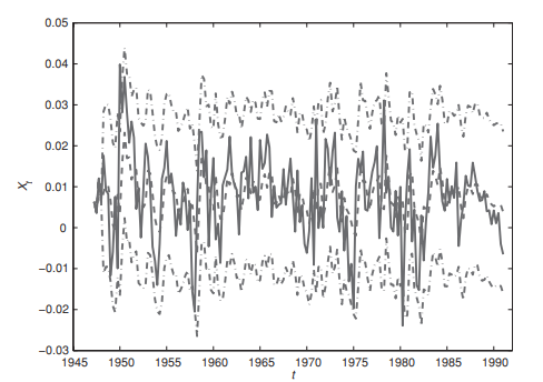
Example 3.11: In the Australian rainfall example, Markov chains of orders $r=2$ and 3 were considered. In each case, $\operatorname{Be}(1 / 2,1 / 2)$ priors were used for the first nonzero element of each row of the transition matrix and it was assumed that the initial $r$ states were generated from the equilibrium distribution. Then, the predictive equilibrium probabilities of the different states under each model are as follows
The log marginal likelihoods are $-30.7876$ for the second-order model and $-32.1915$ for the third-order model, respectively, which suggest that the simple Markov chain model should be preferred.
Bayesian inference for the MTD model of (3.1) is also straightforward. Assume first that the order $r$ of the Markov chain mixture is known. Then, defining an indicator variable $Z_{n}$ such that $P\left(Z_{n}=z \mid \mathbf{w}\right)=w_{z}$, observe that the mixture transition model can be represented as
$$
P\left(X_{n}=x_{n} \mid X_{n-1}=x_{n-1}, \ldots, X_{n-r}=x_{n-r}, Z_{n}=z, P\right)=p_{x_{n-z} x_{n}}
$$
Then, a posteriori,
$$
P\left(Z_{n}=z \mid X_{n}=x_{n}, \ldots, X_{n-r}=x_{n-r}, Z_{n}=z, \boldsymbol{P}\right)=\frac{w_{z} p_{x_{n-z} x_{n}}}{\sum_{j=1}^{r} w_{j} p_{x_{n-j} x_{n}}}
$$
Now, define the usual matrix beta prior for $\boldsymbol{P}$, a Dirichlet prior for $\mathbf{w}$, say $\mathbf{w} \sim \operatorname{Dir}\left(\beta_{1}, \ldots, \beta_{r}\right)$, and a probability model $P\left(x_{0}, \ldots, x_{r-1}\right)$ for the initial states of the chain. Then given a sequence of data, $\mathbf{x}=\left(x_{0}, \ldots, x_{n}\right)$, if the indicator variables are $\mathbf{z}=\left(z_{r}, \ldots, z_{n}\right)$ then
$$
\begin{aligned}
f(\boldsymbol{P} \mid \mathbf{x}, \mathbf{z}, \mathbf{w}) &=\prod_{t=r}^{n} p_{x_{t-z_{t}} x_{t}} f(\boldsymbol{P}) \
f(\mathbf{w} \mid \mathbf{z}) &=\prod_{t=r}^{n} w_{z_{t}} f(\mathbf{w}),
\end{aligned}
$$
which are matrix beta and Dirichlet distributions, respectively. Therefore, a simple Gibbs sampling algorithm can be set up to sample the posterior distribution of $\mathbf{w}, \boldsymbol{P}$ by successively sampling from (3.6), (3.7), and (3.7).
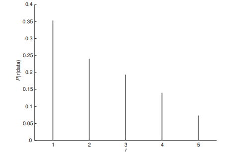
When the order of the chain is unknown, two approaches might be considered. First, models of different orders could be fitted and then Bayes factors could be used for model selection as in Section 3.3.5. Otherwise a prior distribution can be defined over the different orders and then a variable dimension MCMC algorithm such as reversible jump (Green, 1995, Richardson and Green 1997) could be used to evaluate the posterior distribution, as in the following example.
随机过程代写
统计代写|应用随机过程代写Stochastic process代考|Partially observed data
现在假设马尔可夫链仅在多个有限时间点被观察到。例如,假设X0是一个已知的初始状态,我们观察到X这=(Xn1,…,Xn米), 在哪里n1<…<n米∈ñ. 在这种情况下,似然函数是
一世(磷∣X这)=∏一世=1米pn一世−1n一世−吨一世−1)(l一世)
在哪里p一世j(吨)代表(一世,j)的第一个元素吨步骤转换矩阵,在第 1.3.1 节中定义。在许多情况下,这种可能性的计算会很复杂。因此,通常最好考虑基于缺失观测值的重构进行推理。让X米有时代表未观察到的状态1,…, 吨1−1,吨1+1,…,吨n−1−1,吨n−1+1,…,吨n然后让X表示完整的数据序列。然后,给定一个矩阵 beta,我们有磷∣X也是矩阵 beta。此外,立即
磷(X米∣X这,磷)=磷(X∣磷)磷(X这∣磷)∝磷(X∣磷),对于给定的,这很容易计算磷,X米. 一种可能性是在 Gibbs 采样算法中建立一个 Metropolis,以从磷.
如果丢失的数据量相对较小,这种方法是合理的。但是,如果有很多缺失的数据,则很难定义一个合适的算法来生成数据磷(X米∣X这,磷)在(3.5)中。在这种情况下,一种可能性是生成X米一个接一个,使用单独的 Gibbs 步骤。因此,如果吨是与缺失观察相关的时间中的一个时间点,那么我们可以生成一个状态X吨使用
磷(X吨∣X−F,磷)∝pX吨−1X吨pX吨X吨+1
在哪里X−吨表示除时间状态外的完整状态序列吨.
统计代写|应用随机过程代写Stochastic process代考|Reversible Markov chains
假设我们有一个具有未知转移矩阵的可逆马尔可夫链磷和均衡分布圆周率满足定义 3.1 的条件。然后,对于观察一系列观察的标准实验,X0,…,Xn,从链上,其中初始状态X0假设已知,共轭先验分布可以如下推导。
首先,链表示为图,G, 有顶点在和边缘和, 使得两个顶点一世和j由一条边连接,和=一世,j, 当且仅当p一世j>0和边缘和∈和被加权,因此,对于和=一世,j,在和∝圆周率(一世)p一世j=圆周率(j)pj一世和∑和∈和在和=1. 请注意,如果p一世一世>0,则有对应的边,和=一世,一世称为循环。循环集应表示为和环形。 .
可逆马尔可夫链的共轭概率分布现在可以定义为权重分布,在如下。对于一个边缘和∈和, 让和¯代表端点和; 对于一个顶点在∈在, 放在在=∑和:在∈和¯在C. 另外,定义吨是生成树的集合G,即包含所有循环的最大子图集G,但没有循环。对于生成树,吨∈吨, 让和(吨)表示边集吨. 然后,共轭先验分布为在是(谁)给的:
F(在∣在0,一种)∝∏和∈和∖和丢失 在和一种和−1/2∏和∈和种族 在和一种和/2−1在在0一种在0/2∏在∈在∖在0在在(一种在+1)/2∑吨∈吨∏和∉和(吨)1在C
在哪里在0表示对应于初始状态的图的节点,X0, 一种=(一种和)和∈和是任意非负常数的矩阵,并且一种在=∑和:在∈和¯一种和.
后验分布是F(在∣X)=F(在∣在n,一种′), 在哪里一种′=(一种和+ķ和(X))和∈和和 $$ k{e}(\mathbf{x})=\left{\begin{对齐} \left|\left{i \in{1, \ldots, n}:\left{x_{i-1}, x_{i}\right}=e\right}\right|, & \text { for } e \in E \反斜杠 E_{\text {loop }} \ 2\left|\left{i \in{1, \ldots, n}:\left{x_{i-1}, x_ {i}\right}=e\right}\right|, & \text { for } e \in E_{\text {loop }} \end{aligned}\begin{对齐} \left|\left{i \in{1, \ldots, n}:\left{x_{i-1}, x_{i}\right}=e\right}\right|, & \text { for } e \in E \反斜杠 E_{\text {loop }} \ 2\left|\left{i \in{1, \ldots, n}:\left{x_{i-1}, x_ {i}\right}=e\right}\right|, & \text { for } e \in E_{\text {loop }} \end{aligned}\对。
$$
在哪里|⋅|表示集合的基数。因此,对于一个边和这不是一个循环,ķ和(X)表示遍历的次数和由路径X=(X0,X1,…,Xn)对于一个循环,ķ和(X)是遍历次数的两倍和.
分布的积分常数和矩是已知的,可以直接从后验分布进行模拟;有关详细信息,请参阅 Diaconis 和 Rolles (2006)。
统计代写|应用随机过程代写Stochastic process代考|Higher order chains and mixtures of Markov chains
完整的贝叶斯推理r原则上,三阶马尔可夫链模型可以与一阶模型的推理完全相同,通过适当地扩展状态数量,如第 3.2.2 节所述。
示例 3.11:在澳大利亚降雨示例中,马尔可夫订单链r=2并考虑了3个。在每种情况下,是(1/2,1/2)先验用于转换矩阵每一行的第一个非零元素,并假设初始r状态是从平衡分布产生的。则各模型下不同状态的预测均衡概率如下
对数边际似然是−30.7876对于二阶模型和−32.1915对于三阶模型,这表明应该首选简单的马尔可夫链模型。
(3.1) 的 MTD 模型的贝叶斯推理也很简单。首先假设订单r马尔可夫链混合物是已知的。然后,定义一个指示变量从n这样磷(从n=和∣在)=在和,观察混合过渡模型可以表示为
磷(Xn=Xn∣Xn−1=Xn−1,…,Xn−r=Xn−r,从n=和,磷)=pXn−和Xn
然后,事后,
磷(从n=和∣Xn=Xn,…,Xn−r=Xn−r,从n=和,磷)=在和pXn−和Xn∑j=1r在jpXn−jXn
现在,定义通常的矩阵 beta 先验磷, Dirichlet 先验在, 说在∼目录(b1,…,br), 和一个概率模型磷(X0,…,Xr−1)对于链的初始状态。然后给定一个数据序列,X=(X0,…,Xn), 如果指标变量是和=(和r,…,和n)然后
F(磷∣X,和,在)=∏吨=rnpX吨−和吨X吨F(磷) F(在∣和)=∏吨=rn在和吨F(在),
分别是矩阵 beta 和 Dirichlet 分布。因此,可以建立一个简单的 Gibbs 采样算法来采样在,磷通过从 (3.6)、(3.7) 和 (3.7) 中连续采样。
当链的顺序未知时,可以考虑两种方法。首先,可以拟合不同阶数的模型,然后可以使用贝叶斯因子进行模型选择,如第 3.3.5 节所述。否则,可以在不同阶数上定义先验分布,然后可以使用可变维度 MCMC 算法,例如可逆跳跃(Green,1995,Richardson 和 Green 1997)来评估后验分布,如下例所示。

统计代写请认准statistics-lab™. statistics-lab™为您的留学生涯保驾护航。
金融工程代写
金融工程是使用数学技术来解决金融问题。金融工程使用计算机科学、统计学、经济学和应用数学领域的工具和知识来解决当前的金融问题,以及设计新的和创新的金融产品。
非参数统计代写
非参数统计指的是一种统计方法,其中不假设数据来自于由少数参数决定的规定模型;这种模型的例子包括正态分布模型和线性回归模型。
广义线性模型代考
广义线性模型(GLM)归属统计学领域,是一种应用灵活的线性回归模型。该模型允许因变量的偏差分布有除了正态分布之外的其它分布。
术语 广义线性模型(GLM)通常是指给定连续和/或分类预测因素的连续响应变量的常规线性回归模型。它包括多元线性回归,以及方差分析和方差分析(仅含固定效应)。
有限元方法代写
有限元方法(FEM)是一种流行的方法,用于数值解决工程和数学建模中出现的微分方程。典型的问题领域包括结构分析、传热、流体流动、质量运输和电磁势等传统领域。
有限元是一种通用的数值方法,用于解决两个或三个空间变量的偏微分方程(即一些边界值问题)。为了解决一个问题,有限元将一个大系统细分为更小、更简单的部分,称为有限元。这是通过在空间维度上的特定空间离散化来实现的,它是通过构建对象的网格来实现的:用于求解的数值域,它有有限数量的点。边界值问题的有限元方法表述最终导致一个代数方程组。该方法在域上对未知函数进行逼近。[1] 然后将模拟这些有限元的简单方程组合成一个更大的方程系统,以模拟整个问题。然后,有限元通过变化微积分使相关的误差函数最小化来逼近一个解决方案。
tatistics-lab作为专业的留学生服务机构,多年来已为美国、英国、加拿大、澳洲等留学热门地的学生提供专业的学术服务,包括但不限于Essay代写,Assignment代写,Dissertation代写,Report代写,小组作业代写,Proposal代写,Paper代写,Presentation代写,计算机作业代写,论文修改和润色,网课代做,exam代考等等。写作范围涵盖高中,本科,研究生等海外留学全阶段,辐射金融,经济学,会计学,审计学,管理学等全球99%专业科目。写作团队既有专业英语母语作者,也有海外名校硕博留学生,每位写作老师都拥有过硬的语言能力,专业的学科背景和学术写作经验。我们承诺100%原创,100%专业,100%准时,100%满意。
随机分析代写
随机微积分是数学的一个分支,对随机过程进行操作。它允许为随机过程的积分定义一个关于随机过程的一致的积分理论。这个领域是由日本数学家伊藤清在第二次世界大战期间创建并开始的。
时间序列分析代写
随机过程,是依赖于参数的一组随机变量的全体,参数通常是时间。 随机变量是随机现象的数量表现,其时间序列是一组按照时间发生先后顺序进行排列的数据点序列。通常一组时间序列的时间间隔为一恒定值(如1秒,5分钟,12小时,7天,1年),因此时间序列可以作为离散时间数据进行分析处理。研究时间序列数据的意义在于现实中,往往需要研究某个事物其随时间发展变化的规律。这就需要通过研究该事物过去发展的历史记录,以得到其自身发展的规律。
回归分析代写
多元回归分析渐进(Multiple Regression Analysis Asymptotics)属于计量经济学领域,主要是一种数学上的统计分析方法,可以分析复杂情况下各影响因素的数学关系,在自然科学、社会和经济学等多个领域内应用广泛。
MATLAB代写
MATLAB 是一种用于技术计算的高性能语言。它将计算、可视化和编程集成在一个易于使用的环境中,其中问题和解决方案以熟悉的数学符号表示。典型用途包括:数学和计算算法开发建模、仿真和原型制作数据分析、探索和可视化科学和工程图形应用程序开发,包括图形用户界面构建MATLAB 是一个交互式系统,其基本数据元素是一个不需要维度的数组。这使您可以解决许多技术计算问题,尤其是那些具有矩阵和向量公式的问题,而只需用 C 或 Fortran 等标量非交互式语言编写程序所需的时间的一小部分。MATLAB 名称代表矩阵实验室。MATLAB 最初的编写目的是提供对由 LINPACK 和 EISPACK 项目开发的矩阵软件的轻松访问,这两个项目共同代表了矩阵计算软件的最新技术。MATLAB 经过多年的发展,得到了许多用户的投入。在大学环境中,它是数学、工程和科学入门和高级课程的标准教学工具。在工业领域,MATLAB 是高效研究、开发和分析的首选工具。MATLAB 具有一系列称为工具箱的特定于应用程序的解决方案。对于大多数 MATLAB 用户来说非常重要,工具箱允许您学习和应用专业技术。工具箱是 MATLAB 函数(M 文件)的综合集合,可扩展 MATLAB 环境以解决特定类别的问题。可用工具箱的领域包括信号处理、控制系统、神经网络、模糊逻辑、小波、仿真等。