如果你也在 怎样代写数据可视化Data visualization这个学科遇到相关的难题,请随时右上角联系我们的24/7代写客服。
数据可视化是将信息转化为视觉背景的做法,如地图或图表,使数据更容易被人脑理解并从中获得洞察力。数据可视化的主要目标是使其更容易在大型数据集中识别模式、趋势和异常值。
statistics-lab™ 为您的留学生涯保驾护航 在代写数据可视化Data visualization方面已经树立了自己的口碑, 保证靠谱, 高质且原创的统计Statistics代写服务。我们的专家在代写数据可视化Data visualization代写方面经验极为丰富,各种代写数据可视化Data visualization相关的作业也就用不着说。
我们提供的数据可视化Data visualization及其相关学科的代写,服务范围广, 其中包括但不限于:
- Statistical Inference 统计推断
- Statistical Computing 统计计算
- Advanced Probability Theory 高等概率论
- Advanced Mathematical Statistics 高等数理统计学
- (Generalized) Linear Models 广义线性模型
- Statistical Machine Learning 统计机器学习
- Longitudinal Data Analysis 纵向数据分析
- Foundations of Data Science 数据科学基础
统计代写|数据可视化代写Data visualization代考|Figures should be Aesthetically Appropriate
It’s surprisingly common to see figures that are pixelated, whose labels are too small (or too large) relative to the text, or whose font family is inconsistent with the text. Another common issue (especially in presentations) is the choice of colors: if you have a dark background in your figure, the choice of colors must take that into account, otherwise it will be much harder for the audience to read your slides-especially considering that projectors often don’t have great contrast and resolution.
Your figures should look crisp even when you zoom in, and they should not distract the reader from what really matters (again: less is more). You should have clear labels along the axes (when needed) and an informative caption, and your use of color should serve a purpose-remember that using colors can actually be a problem in some journals. In reality, it’s usually possible to remove the colors from a figure and use some other dimension to convey the same information-we will exercise that throughout the book.
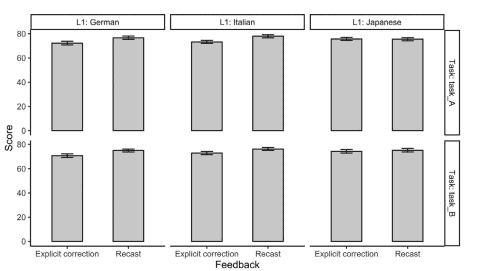
Fig. 2.4, like the figure we discussed earlier in this chapter (Fig. 2.3), shows a bar plot. Here, however, we have three dimensions: the $y$-axis shows the change in score (e.g., pre- and post-test) of the hypothetical study mentioned earlier; the $x$-axis shows the different native languages of the participants in said study; and the fill of the bars discriminates the two methods under examination. Note that the font sizes are appropriate (not too small, not too large). In addition, the key is positioned at the top of the figure, not at the side. This allows us to better use the space (i.e., increase the horizontal size of the figure itself). No colors are needed here, since the fill of the bars represents a factor with only two levels (“In-person” and “Online”). Finally, the bars represent the mean improvement, but the plot also shows standard errors from the mean. If the plot only showed means, it would be considerably less informative, as we would know nothing about how certain we are about the means in question (i.e., we would not incorporate information about the variance in the data).
统计代写|数据可视化代写Data visualization代考|Basic Statistics in R
So far in this chapter we have covered a lot. We installed $\mathrm{R}$ and RStudio, discussed RStudio’s interface, and explored some $R$ basics with a number of code blocks, which led us to ggplot2 and figures in the previous section. Once we have a figure, the natural next step is to statistically analyze the patterns shown in said figure. Thus, in this section of the chapter, we will turn to some basic statistical concepts-this will be a good opportunity to review some concepts that will be used throughout the book. We’ll first start with one of the most basic concepts, namely, sampling.
Assume we want to collect data on proficiency scores from 20 learners. To simulate an entire population of learners containing, say, 1 million data points, we can use the function rnorm(), which randomly generates numbers following a normal (Gaussian) distribution ${ }^{25}$ (there’s no reason to assume that proficiency scores are not normally distributed here). Create a variable called pop and assign to it $\operatorname{rnorm}(\mathrm{n}=1000000$, mean $=85, \mathrm{sd}=8)$-you can even do this in the console, without creating a new script, since it will be a simple exercise. This will generate one million scores normally distributed around a mean $(\mu)$ of 85 points with a standard deviation $(\sigma)$ of 8 points. In reality, we never know what the mean and standard deviations are for our population, but here we do since we are the ones simulating the data. You can check that both $\mu$ and $\sigma$ are roughly 85 and 8 , respectively, by running mean(pop) and sd(pop) you won’t get exact numbers, but they should be very close to the parameter values we set using rnorm().
Next, let’s sample 20 values from pop-this is equivalent to collecting data from 20 learners from a population of one million learners. To do that, create a new variable, sam, and assign to it sample $(x=$ pop, size $=20)$. Now, run mean( ) and sd() on sam, and you should get a sample mean $(\bar{x})$ and a sample standard deviation $(s)$ that should be very similar to the true population parameters $(\mu, \sigma)$ we defined earlier. This is a quick and easy way to see sampling at work: we define the population ourselves, so it’s straightforward to check how representative our sample is.
统计代写|数据可视化代写Data visualization代考|What’s Your Research Question
If you already have actual data, that means you have long passed the stages of formulating a research question and working on your study design. Having a relevant research question is as important as it is difficult-see Mackey and Gass (2016, ch. 1). Great studies are in part the result of great research questions. Your question will dictate how you will design your study, which in turn will dictate how you will analyze your data. Understanding all three components is essential. After all, you may have an interesting question but fail to have an adequate study design, or you may have both a relevant question and an appropriate study design but realize that you don’t know how to analyze the data.
The hypothetical dataset in question (long) consists of two groups of participants (control and target) as well as three sets of test scores-we will examine more complex and realistic datasets later on, but for now our tibble long will be sufficient. Suppose that our study examines the effects of a particular pedagogical approach on students’ scores, as briefly mentioned earlier. For illustrative purposes, let’s assume that we want to compare a student-centered approach (e.g., workshop-based), our targets (treatment group), to a teacher-centered approach (e.g., lecture-based), our controls, so we are comparing two clearly defined approaches (two groups). Next, we must be able to measure scores. To do that, we have decided to administer three tests (e.g., a pre-test (testA), a post-test (testB), and a delayed post-test (testC), as alluded to earlier). With that in mind, we can ask specific questions: is the improvement from test $A$ to testB statistically different between controls and targets? How about from testA to testC? These questions must speak directly to your overarching research question. Finally, in addition to a research question, you may have a directional hypothesis, for example, that a lecture-based approach will lead to lower scores overall, or a non-directional hypothesis, for example, that there will be some difference in learning between the two approaches, but which one will be better is unknown. Let’s now go over some basic stats assuming the hypothetical context in question.
数据可视化代考
统计代写|数据可视化代写Data visualization代考|Figures should be Aesthetically Appropriate
看到像素化的图形,其标签相对于文本太小(或太大),或者其字体系列与文本不一致的情况令人惊讶地常见。另一个常见的问题(尤其是在演示文稿中)是颜色的选择:如果你的图形中有深色背景,颜色的选择必须考虑到这一点,否则观众阅读你的幻灯片会更加困难——尤其是考虑到投影仪通常没有很好的对比度和分辨率。
即使放大,您的数字也应该看起来很清晰,并且它们不应该分散读者对真正重要的事情的注意力(再次:少即是多)。您应该在轴上(需要时)有清晰的标签和信息性标题,并且您对颜色的使用应该有目的 – 请记住,在某些期刊中使用颜色实际上可能是一个问题。实际上,通常可以从图形中去除颜色并使用其他维度来传达相同的信息——我们将在整本书中练习。
图 2.4 与我们在本章前面讨论的图(图 2.3)一样,显示了一个条形图。然而,在这里,我们有三个维度:是-轴显示前面提到的假设研究的分数变化(例如,测试前和测试后);这X-轴显示所述研究参与者的不同母语;并且条形的填充区分了正在检查的两种方法。注意字体大小合适(不要太小,不要太大)。此外,钥匙位于图的顶部,而不是侧面。这使我们可以更好地利用空间(即增加图形本身的水平尺寸)。这里不需要颜色,因为条形的填充表示一个只有两个级别(“面对面”和“在线”)的因素。最后,条形代表平均改进,但该图还显示了均值的标准误差。如果该图仅显示均值,则信息量将大大减少,因为我们对所讨论的均值的确定程度一无所知(即,我们不会在数据中包含有关方差的信息)。
统计代写|数据可视化代写Data visualization代考|Basic Statistics in R
到目前为止,我们已经在本章中介绍了很多内容。我们安装了R和 RStudio,讨论了 RStudio 的界面,并探索了一些R带有许多代码块的基础知识,这使我们了解了上一节中的 ggplot2 和图形。一旦我们有了一个图形,下一步自然是对所述图形中显示的模式进行统计分析。因此,在本章的这一部分,我们将转向一些基本的统计概念——这将是一个很好的机会来回顾将在整本书中使用的一些概念。我们首先从最基本的概念之一开始,即采样。
假设我们要收集 20 名学习者的熟练度分数数据。为了模拟包含 100 万个数据点的整个学习者群体,我们可以使用函数 rnorm(),它随机生成服从正态(高斯)分布的数字25(没有理由假设熟练度分数在这里不是正态分布的)。创建一个名为 pop 的变量并分配给它规范(n=1000000, 意思是=85,sd=8)-您甚至可以在控制台中执行此操作,而无需创建新脚本,因为这将是一个简单的练习。这将产生一百万个正态分布在平均值附近的分数(μ)85分,标准差(σ)8 分。实际上,我们永远不知道我们的人口的均值和标准差是多少,但在这里我们知道,因为我们是模拟数据的人。您可以检查两者μ和σ分别大约是 85 和 8 ,通过运行 mean(pop) 和 sd(pop) 你不会得到确切的数字,但它们应该非常接近我们使用 rnorm() 设置的参数值。
接下来,让我们从 pop 中抽取 20 个值——这相当于从 100 万学习者的人口中收集了 20 个学习者的数据。为此,创建一个新变量 sam,并将其分配给 sample(X=流行,大小=20). 现在,在 sam 上运行 mean() 和 sd(),你应该得到一个样本均值(X¯)和样本标准差(s)这应该与真实的人口参数非常相似(μ,σ)我们之前定义的。这是查看工作中抽样的一种快速简便的方法:我们自己定义总体,因此可以直接检查我们的样本的代表性。
统计代写|数据可视化代写Data visualization代考|What’s Your Research Question
如果您已经拥有实际数据,这意味着您早已通过了制定研究问题和研究设计的阶段。有一个相关的研究问题与它一样重要 – 见 Mackey 和 Gass (2016, ch. 1)。伟大的研究部分是伟大研究问题的结果。您的问题将决定您将如何设计您的研究,而这反过来又将决定您将如何分析您的数据。了解所有三个组成部分是必不可少的。毕竟,您可能有一个有趣的问题但没有足够的研究设计,或者您可能既有相关的问题又有适当的研究设计,但意识到您不知道如何分析数据。
有问题的假设数据集(长)由两组参与者(控制组和目标组)以及三组测试分数组成——我们稍后会检查更复杂和现实的数据集,但现在我们的 tibble long 就足够了。假设我们的研究检查了特定教学方法对学生成绩的影响,如前所述。为了说明的目的,假设我们想要比较以学生为中心的方法(例如,基于研讨会),我们的目标(治疗组),以教师为中心的方法(例如,基于讲座),我们的控制,所以我们正在比较两种明确定义的方法(两组)。接下来,我们必须能够衡量分数。为此,我们决定管理三个测试(例如,前测 (testA)、后测 (testB) 和延迟后测 (testC),如前所述)。考虑到这一点,我们可以提出具体的问题:测试的改进一个testB 控制和目标之间的统计差异?从 testA 到 testC 怎么样?这些问题必须直接针对您的总体研究问题。最后,除了一个研究问题,你可能有一个方向性假设,例如,基于讲座的方法会导致整体得分较低,或者一个非方向性假设,例如,学习会有一些差异在这两种方法之间,但哪种方法更好还不得而知。现在让我们在假设的假设背景下回顾一些基本统计数据。

统计代写请认准statistics-lab™. statistics-lab™为您的留学生涯保驾护航。
金融工程代写
金融工程是使用数学技术来解决金融问题。金融工程使用计算机科学、统计学、经济学和应用数学领域的工具和知识来解决当前的金融问题,以及设计新的和创新的金融产品。
非参数统计代写
非参数统计指的是一种统计方法,其中不假设数据来自于由少数参数决定的规定模型;这种模型的例子包括正态分布模型和线性回归模型。
广义线性模型代考
广义线性模型(GLM)归属统计学领域,是一种应用灵活的线性回归模型。该模型允许因变量的偏差分布有除了正态分布之外的其它分布。
术语 广义线性模型(GLM)通常是指给定连续和/或分类预测因素的连续响应变量的常规线性回归模型。它包括多元线性回归,以及方差分析和方差分析(仅含固定效应)。
有限元方法代写
有限元方法(FEM)是一种流行的方法,用于数值解决工程和数学建模中出现的微分方程。典型的问题领域包括结构分析、传热、流体流动、质量运输和电磁势等传统领域。
有限元是一种通用的数值方法,用于解决两个或三个空间变量的偏微分方程(即一些边界值问题)。为了解决一个问题,有限元将一个大系统细分为更小、更简单的部分,称为有限元。这是通过在空间维度上的特定空间离散化来实现的,它是通过构建对象的网格来实现的:用于求解的数值域,它有有限数量的点。边界值问题的有限元方法表述最终导致一个代数方程组。该方法在域上对未知函数进行逼近。[1] 然后将模拟这些有限元的简单方程组合成一个更大的方程系统,以模拟整个问题。然后,有限元通过变化微积分使相关的误差函数最小化来逼近一个解决方案。
tatistics-lab作为专业的留学生服务机构,多年来已为美国、英国、加拿大、澳洲等留学热门地的学生提供专业的学术服务,包括但不限于Essay代写,Assignment代写,Dissertation代写,Report代写,小组作业代写,Proposal代写,Paper代写,Presentation代写,计算机作业代写,论文修改和润色,网课代做,exam代考等等。写作范围涵盖高中,本科,研究生等海外留学全阶段,辐射金融,经济学,会计学,审计学,管理学等全球99%专业科目。写作团队既有专业英语母语作者,也有海外名校硕博留学生,每位写作老师都拥有过硬的语言能力,专业的学科背景和学术写作经验。我们承诺100%原创,100%专业,100%准时,100%满意。
随机分析代写
随机微积分是数学的一个分支,对随机过程进行操作。它允许为随机过程的积分定义一个关于随机过程的一致的积分理论。这个领域是由日本数学家伊藤清在第二次世界大战期间创建并开始的。
时间序列分析代写
随机过程,是依赖于参数的一组随机变量的全体,参数通常是时间。 随机变量是随机现象的数量表现,其时间序列是一组按照时间发生先后顺序进行排列的数据点序列。通常一组时间序列的时间间隔为一恒定值(如1秒,5分钟,12小时,7天,1年),因此时间序列可以作为离散时间数据进行分析处理。研究时间序列数据的意义在于现实中,往往需要研究某个事物其随时间发展变化的规律。这就需要通过研究该事物过去发展的历史记录,以得到其自身发展的规律。
回归分析代写
多元回归分析渐进(Multiple Regression Analysis Asymptotics)属于计量经济学领域,主要是一种数学上的统计分析方法,可以分析复杂情况下各影响因素的数学关系,在自然科学、社会和经济学等多个领域内应用广泛。
MATLAB代写
MATLAB 是一种用于技术计算的高性能语言。它将计算、可视化和编程集成在一个易于使用的环境中,其中问题和解决方案以熟悉的数学符号表示。典型用途包括:数学和计算算法开发建模、仿真和原型制作数据分析、探索和可视化科学和工程图形应用程序开发,包括图形用户界面构建MATLAB 是一个交互式系统,其基本数据元素是一个不需要维度的数组。这使您可以解决许多技术计算问题,尤其是那些具有矩阵和向量公式的问题,而只需用 C 或 Fortran 等标量非交互式语言编写程序所需的时间的一小部分。MATLAB 名称代表矩阵实验室。MATLAB 最初的编写目的是提供对由 LINPACK 和 EISPACK 项目开发的矩阵软件的轻松访问,这两个项目共同代表了矩阵计算软件的最新技术。MATLAB 经过多年的发展,得到了许多用户的投入。在大学环境中,它是数学、工程和科学入门和高级课程的标准教学工具。在工业领域,MATLAB 是高效研究、开发和分析的首选工具。MATLAB 具有一系列称为工具箱的特定于应用程序的解决方案。对于大多数 MATLAB 用户来说非常重要,工具箱允许您学习和应用专业技术。工具箱是 MATLAB 函数(M 文件)的综合集合,可扩展 MATLAB 环境以解决特定类别的问题。可用工具箱的领域包括信号处理、控制系统、神经网络、模糊逻辑、小波、仿真等。