如果你也在 怎样代写时间序列分析Time-Series Analysis这个学科遇到相关的难题,请随时右上角联系我们的24/7代写客服。
时间序列分析是分析在一个时间间隔内收集的一系列数据点的具体方式。在时间序列分析中,分析人员在设定的时间段内以一致的时间间隔记录数据点,而不仅仅是间歇性或随机地记录数据点。
statistics-lab™ 为您的留学生涯保驾护航 在代写时间序列分析Time-Series Analysis方面已经树立了自己的口碑, 保证靠谱, 高质且原创的统计Statistics代写服务。我们的专家在代写时间序列分析Time-Series Analysis代写方面经验极为丰富,各种代写时间序列分析Time-Series Analysis相关的作业也就用不着说。
我们提供的时间序列分析Time-Series Analysis及其相关学科的代写,服务范围广, 其中包括但不限于:
- Statistical Inference 统计推断
- Statistical Computing 统计计算
- Advanced Probability Theory 高等概率论
- Advanced Mathematical Statistics 高等数理统计学
- (Generalized) Linear Models 广义线性模型
- Statistical Machine Learning 统计机器学习
- Longitudinal Data Analysis 纵向数据分析
- Foundations of Data Science 数据科学基础
统计代写|时间序列分析代写Time-Series Analysis代考|Basic Statistical Characteristics
The notation used in this book for time series is $x_{t}, t=\Delta t, \ldots, N \Delta t$, where $N$ is the number of terms in the time series and $\Delta t$ is the time interval between consecutive terms. The sampling rate is the number of samples per unit time and, as a rule, the sampling rate here is one sample per year or one sample per month, that is, $\Delta t=1$ year or $\Delta t=1$ month. The notation for the time series can also be given as $x_{t}, t=1, \ldots, N$ having in mind that $\Delta t=1$. In what follows, the time series is considered as long if its length exceeds the largest time scale of interest by orders of magnitude. Otherwise, the time series has to be treated as short.
A major characteristic of a time series is its probability density function $p(x)$, which defines the probability of encountering different numerical values of $x_{t}$. The common abbreviation for $p(x)$ is PDF. The PDF of a scalar time series is characterized with its statistical moments, or statistics, such as mean value and variance (central moments), covariance function and spectral density (mixed moments), and with higher central moments such as skewness and kurtosis.
There are many different types of PDFs, but the function which is most important for practical time series analysis (if its application can be justified for a given time series) is the Gaussian or normal, probability density function
$$
p\left(x_{t}\right)=\frac{1}{\sigma_{x} \sqrt{2 \pi}} \exp \left[-\left(x_{t}-\bar{x}\right)^{2} / 2 \sigma_{x}^{2}\right]
$$
where the mean value
$$
\bar{x}=\lim {N \rightarrow \infty} \frac{1}{N} \sum{t=1}^{N} x_{t}
$$
and
$$
\sigma_{x}^{2}=\lim {N \rightarrow \infty} \frac{1}{N} \sum{t=1}^{N}\left(x_{t}-\bar{x}\right)^{2}
$$
is the variance of the time series. The positive square root $\sigma_{x}$ of the variance is called the root mean square (RMS) value or standard deviation. The variance (and RMS) describes the variability of the process: a larger variance means a larger dynamic range of numerical values of the process. These definitions are true for random functions of time and for sequences of time-invariant random variables. The Gaussian PDF of random variables is completely described with the mean value $\bar{x}$ and the variance $\sigma_{x}^{2}$. By default, it is generally assumed here that time series are generated by Gaussian (normally distributed) random processes. This assumption does not limit or degrades the properties and abilities of the methods used in this book for time series analysis because the Gaussian probability distribution means the best possible results in all cases when the method is linear. The analysis of non-Gaussian time series requires estimation of the same statistical characteristics as in the Gaussian case and then some higher statistical moments. The methods applied here are linear, and they cover all traditional tasks of time series analysis, including spectral estimation and statistical (probabilistic) forecasting. The normal hypothesis should always be tested for the actual time series that is being analyzed.
The skewness and kurtosis can be helpful for analyzing geophysical and solar time series as measures of PDF’s asymmetry and tail properties, respectively. They are mostly used for determining whether the PDF is close enough to a Gaussian (normal) distribution. Specifically, if the absolute values of standardized skewness and standardized kurtosis do not exceed 2 , the time series can be generally regarded as Gaussian. (Standardized skewness and kurtosis are found by dividing respective estimate by $\sqrt{6 / N}$ and by $\sqrt{24 / N}$ ).
The PDFs and their central statistical moments completely describe properties of sets of random variables, which do not depend upon the time argument. In contrast to random vectors, time series present samples of random processes and their description is not possible without mixed statistical moments such as covariance and correlation functions in the time domain and the spectral density in the frequency domain. These functions are defined in Sect. 2.4.
统计代写|时间序列分析代写Time-Series Analysis代考|Deterministic Process
In contrast to time series consisting of random variables, one can imagine a time-dependent process that follows a specific mathematical law, which excludes any randomness. Respective data present a deterministic process. Deterministic phenomena or processes can be predicted at any lead time without an error.
At climatic time scales (longer than one year), the only geophysical processes that can be regarded as deterministic are those that are caused by astronomical factors. With one exception (a barely detectible tidal harmonic with period of 18.61 years), the time scales of such processes extend to millennia and longer (e.g., Monin 1986) and their effects upon climate at the practically important time scales of year-toyear variability, decades and centuries are negligibly small. At smaller time scales, the only deterministic process in the Earth system is tides, which can be predicted practically precisely in the open ocean and along most shorelines. With the exception of solar and lunar tides, all other geophysical and relevant solar processes are random. Moreover, in some coastal areas (e.g., Newlyn, UK), the sea level variations can be better predicted in a different manner, “without astronomical prejudice and fully allowing for the presence of noise” (Munk and Cartwright 1966). An earlier method of tidal prediction without tidal harmonics had been developed by A. Duvanin $(1960)$.
统计代写|时间序列分析代写Time-Series Analysis代考|Random Process
A random (stochastic, probabilistic) process is any process running in time and controlled by probabilistic laws (Doob 1953). A random process consists of an infinite set of all possible sample records (time series, random functions of time) generated supposedly as the results of repeated experiments or observations. The random processes discussed here are always discreet, that is, the time argument takes only discrete values.
There are two major types of random processes: stationary and nonstationary. A stationary process is the process whose statistical properties determined by averaging at different time origins over the infinite set of sample records of the process do not depend upon the time origin. A nonstationary process does not possess this property.
The time series studied in this book belong to the class of stationary random processes.
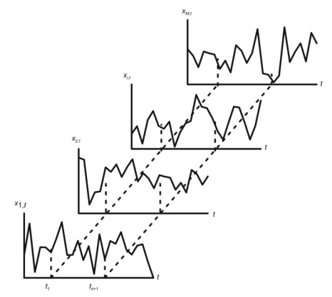
Consider this concept using the mean value and variance as examples. Let $x_{i, t}, i=$ $1, \ldots, M ; t=1, \ldots, N$ be an ensemble of sample records of a random process as shown in Fig. 2.1.
The mean value (or mathematical expectation) $\hat{x}(t)$ at time $t$ is defined as the limit of the sum of $M$ values of $x_{i, t}$ at time $t$ divided by the number of sample records $M$ as $M$ tends to infinity:
$$
\hat{x}(t)=\lim {M \rightarrow \infty} \frac{1}{M} \sum{i=1}^{M} x_{i, t} .
$$
A random process is stationary with respect to the mean value if the mean values $\hat{x}(t)$ are statistically the same for all $t$.
If it is also true that the variance
$$
\hat{\sigma}{x}^{2}(t)=\lim {M \rightarrow \infty} \frac{1}{M} \sum_{i=1}^{M}\left[x_{i, t}-\hat{x}(t)\right]^{2}
$$
of the process possesses the same property, that is, it takes statistically the same value for all $t$, then we have a second order stationary random process.
According to the above definition, one sample record (time series) is not sufficient for studying a random process. This statement is true even if the sample record is known on the entire time axis from $-\infty$ to $+\infty$. Therefore, studying a random process requires a set of sample records (theoretically, an infinite set), so that all characteristics of the process (i.e., its PDF and its statistical moments) are determined by averaging over the ensemble of sample records. This cannot happen in geophysics in general, in climatology, or in solar physics where many if not all time series are unique. Therefore, by studying a single sample record of a stationary random process and extending the results of analysis to the entire process, one assumes by default that the results obtained by analyzing its properties through averaging over time coincide with the results of averaging over an ensemble of such records at different time origins. A random process that possesses this property is called ergodic. An ergodic process is always stationary.
时间序列分析代考
统计代写|时间序列分析代写Time-Series Analysis代考|Basic Statistical Characteristics
本书中用于时间序列的符号是X吨,吨=Δ吨,…,ñΔ吨, 在哪里ñ是时间序列中的项数,并且Δ吨是连续词之间的时间间隔。抽样率是单位时间内的样本数,这里的抽样率通常是每年一个样本或每月一个样本,即Δ吨=1年或Δ吨=1月。时间序列的符号也可以表示为X吨,吨=1,…,ñ考虑到Δ吨=1. 在下文中,如果时间序列的长度超过感兴趣的最大时间尺度几个数量级,则时间序列被认为是长的。否则,时间序列必须被视为短。
时间序列的一个主要特征是它的概率密度函数p(X),它定义了遇到不同数值的概率X吨. 常见的缩写p(X)是PDF。标量时间序列的 PDF 的特征在于其统计矩或统计量,例如平均值和方差(中心矩)、协方差函数和谱密度(混合矩),以及更高的中心矩,例如偏度和峰度。
有许多不同类型的 PDF,但对于实际时间序列分析(如果它的应用对于给定的时间序列是合理的)最重要的函数是高斯或正态概率密度函数
p(X吨)=1σX2圆周率经验[−(X吨−X¯)2/2σX2]
其中平均值
X¯=林ñ→∞1ñ∑吨=1ñX吨
和
σX2=林ñ→∞1ñ∑吨=1ñ(X吨−X¯)2
是时间序列的方差。正平方根σX方差的值称为均方根 (RMS) 值或标准差。方差(和 RMS)描述了过程的可变性:方差越大意味着过程数值的动态范围越大。这些定义对于时间的随机函数和时间不变的随机变量序列都是正确的。随机变量的高斯 PDF 完全用均值描述X¯和方差σX2. 默认情况下,这里一般假设时间序列是由高斯(正态分布)随机过程生成的。这个假设不会限制或降低本书中用于时间序列分析的方法的特性和能力,因为高斯概率分布意味着当方法是线性的时,在所有情况下都可能得到最好的结果。非高斯时间序列的分析需要估计与高斯情况相同的统计特征,然后是一些更高的统计矩。这里应用的方法是线性的,它们涵盖了时间序列分析的所有传统任务,包括谱估计和统计(概率)预测。应始终针对正在分析的实际时间序列检验正态假设。
偏度和峰度有助于分析地球物理和太阳时间序列,分别作为 PDF 不对称性和尾部特性的度量。它们主要用于确定 PDF 是否足够接近高斯(正态)分布。具体来说,如果标准化偏度和标准化峰度的绝对值不超过 2 ,则时间序列一般可以认为是高斯的。(标准化偏度和峰度通过将各自的估计除以6/ñ并通过24/ñ ).
PDF 及其中心统计矩完全描述了不依赖于时间参数的随机变量集的属性。与随机向量相比,时间序列呈现随机过程的样本,如果没有混合统计矩(例如时域中的协方差和相关函数以及频域中的谱密度),则无法对其进行描述。这些功能在 Sect 中定义。2.4.
统计代写|时间序列分析代写Time-Series Analysis代考|Deterministic Process
与由随机变量组成的时间序列相比,人们可以想象一个与时间相关的过程,它遵循特定的数学定律,它排除了任何随机性。各个数据呈现确定性过程。可以在任何前置时间预测确定性现象或过程而不会出现错误。
在气候时间尺度上(超过一年),唯一可以被视为确定性的地球物理过程是由天文因素引起的。除了一个例外(几乎无法检测到的潮汐谐波,周期为 18.61 年),这些过程的时间尺度延伸到数千年甚至更长(例如,Monin 1986)及其对气候的影响,它们在逐年变化的实际重要时间尺度上,几十年和几个世纪是微不足道的。在较小的时间尺度上,地球系统中唯一的确定性过程是潮汐,实际上可以在开阔的海洋和大多数海岸线上精确地预测潮汐。除了太阳和月潮之外,所有其他地球物理和相关的太阳过程都是随机的。此外,在一些沿海地区(例如,英国纽林),海平面变化可以用不同的方式更好地预测,“没有天文偏见,完全考虑到噪音的存在”(Munk and Cartwright 1966)。A. Duvanin 开发了一种较早的没有潮汐谐波的潮汐预测方法(1960).
统计代写|时间序列分析代写Time-Series Analysis代考|Random Process
随机(随机、概率)过程是任何在时间上运行并受概率规律控制的过程(Doob 1953)。随机过程由所有可能的样本记录(时间序列、时间的随机函数)的无限集合组成,这些样本记录被认为是重复实验或观察的结果。这里讨论的随机过程总是离散的,也就是说,时间参数只取离散值。
有两种主要类型的随机过程:平稳和非平稳。平稳过程是这样的过程,其统计特性通过在过程的无限组样本记录上的不同时间源处平均确定,不依赖于时间源。非平稳过程不具备此性质。
本书研究的时间序列属于平稳随机过程类。
以平均值和方差为例来考虑这个概念。让X一世,吨,一世= 1,…,米;吨=1,…,ñ是一个随机过程的样本记录的集合,如图 2.1 所示。
平均值(或数学期望)X^(吨)有时吨被定义为总和的极限米的值X一世,吨有时吨除以样本记录数米作为米趋于无穷:
X^(吨)=林米→∞1米∑一世=1米X一世,吨.
一个随机过程相对于平均值是平稳的,如果平均值X^(吨)在统计上对所有人都是相同的吨.
如果方差也是真的
σ^X2(吨)=林米→∞1米∑一世=1米[X一世,吨−X^(吨)]2
的过程具有相同的性质,也就是说,它在统计上对所有吨,那么我们有一个二阶平稳随机过程。
根据上述定义,一个样本记录(时间序列)不足以研究随机过程。即使样本记录在整个时间轴上已知−∞至+∞. 因此,研究一个随机过程需要一组样本记录(理论上是一个无限集),因此过程的所有特征(即它的 PDF 和它的统计矩)都是通过对样本记录的集合进行平均来确定的。这在一般的地球物理学、气候学或太阳物理学中不可能发生,在这些领域中,许多(如果不是全部)时间序列都是独一无二的。因此,通过研究一个平稳随机过程的单个样本记录并将分析结果扩展到整个过程,默认情况下,通过对时间的平均分析其性质所获得的结果与对一个集合的平均结果一致。这样的记录在不同的时间起源。具有此属性的随机过程称为遍历。遍历过程总是静止的。

统计代写请认准statistics-lab™. statistics-lab™为您的留学生涯保驾护航。
金融工程代写
金融工程是使用数学技术来解决金融问题。金融工程使用计算机科学、统计学、经济学和应用数学领域的工具和知识来解决当前的金融问题,以及设计新的和创新的金融产品。
非参数统计代写
非参数统计指的是一种统计方法,其中不假设数据来自于由少数参数决定的规定模型;这种模型的例子包括正态分布模型和线性回归模型。
广义线性模型代考
广义线性模型(GLM)归属统计学领域,是一种应用灵活的线性回归模型。该模型允许因变量的偏差分布有除了正态分布之外的其它分布。
术语 广义线性模型(GLM)通常是指给定连续和/或分类预测因素的连续响应变量的常规线性回归模型。它包括多元线性回归,以及方差分析和方差分析(仅含固定效应)。
有限元方法代写
有限元方法(FEM)是一种流行的方法,用于数值解决工程和数学建模中出现的微分方程。典型的问题领域包括结构分析、传热、流体流动、质量运输和电磁势等传统领域。
有限元是一种通用的数值方法,用于解决两个或三个空间变量的偏微分方程(即一些边界值问题)。为了解决一个问题,有限元将一个大系统细分为更小、更简单的部分,称为有限元。这是通过在空间维度上的特定空间离散化来实现的,它是通过构建对象的网格来实现的:用于求解的数值域,它有有限数量的点。边界值问题的有限元方法表述最终导致一个代数方程组。该方法在域上对未知函数进行逼近。[1] 然后将模拟这些有限元的简单方程组合成一个更大的方程系统,以模拟整个问题。然后,有限元通过变化微积分使相关的误差函数最小化来逼近一个解决方案。
tatistics-lab作为专业的留学生服务机构,多年来已为美国、英国、加拿大、澳洲等留学热门地的学生提供专业的学术服务,包括但不限于Essay代写,Assignment代写,Dissertation代写,Report代写,小组作业代写,Proposal代写,Paper代写,Presentation代写,计算机作业代写,论文修改和润色,网课代做,exam代考等等。写作范围涵盖高中,本科,研究生等海外留学全阶段,辐射金融,经济学,会计学,审计学,管理学等全球99%专业科目。写作团队既有专业英语母语作者,也有海外名校硕博留学生,每位写作老师都拥有过硬的语言能力,专业的学科背景和学术写作经验。我们承诺100%原创,100%专业,100%准时,100%满意。
随机分析代写
随机微积分是数学的一个分支,对随机过程进行操作。它允许为随机过程的积分定义一个关于随机过程的一致的积分理论。这个领域是由日本数学家伊藤清在第二次世界大战期间创建并开始的。
时间序列分析代写
随机过程,是依赖于参数的一组随机变量的全体,参数通常是时间。 随机变量是随机现象的数量表现,其时间序列是一组按照时间发生先后顺序进行排列的数据点序列。通常一组时间序列的时间间隔为一恒定值(如1秒,5分钟,12小时,7天,1年),因此时间序列可以作为离散时间数据进行分析处理。研究时间序列数据的意义在于现实中,往往需要研究某个事物其随时间发展变化的规律。这就需要通过研究该事物过去发展的历史记录,以得到其自身发展的规律。
回归分析代写
多元回归分析渐进(Multiple Regression Analysis Asymptotics)属于计量经济学领域,主要是一种数学上的统计分析方法,可以分析复杂情况下各影响因素的数学关系,在自然科学、社会和经济学等多个领域内应用广泛。
MATLAB代写
MATLAB 是一种用于技术计算的高性能语言。它将计算、可视化和编程集成在一个易于使用的环境中,其中问题和解决方案以熟悉的数学符号表示。典型用途包括:数学和计算算法开发建模、仿真和原型制作数据分析、探索和可视化科学和工程图形应用程序开发,包括图形用户界面构建MATLAB 是一个交互式系统,其基本数据元素是一个不需要维度的数组。这使您可以解决许多技术计算问题,尤其是那些具有矩阵和向量公式的问题,而只需用 C 或 Fortran 等标量非交互式语言编写程序所需的时间的一小部分。MATLAB 名称代表矩阵实验室。MATLAB 最初的编写目的是提供对由 LINPACK 和 EISPACK 项目开发的矩阵软件的轻松访问,这两个项目共同代表了矩阵计算软件的最新技术。MATLAB 经过多年的发展,得到了许多用户的投入。在大学环境中,它是数学、工程和科学入门和高级课程的标准教学工具。在工业领域,MATLAB 是高效研究、开发和分析的首选工具。MATLAB 具有一系列称为工具箱的特定于应用程序的解决方案。对于大多数 MATLAB 用户来说非常重要,工具箱允许您学习和应用专业技术。工具箱是 MATLAB 函数(M 文件)的综合集合,可扩展 MATLAB 环境以解决特定类别的问题。可用工具箱的领域包括信号处理、控制系统、神经网络、模糊逻辑、小波、仿真等。