如果你也在 怎样代写时间序列分析Time-Series Analysis这个学科遇到相关的难题,请随时右上角联系我们的24/7代写客服。
时间序列分析是分析在一个时间间隔内收集的一系列数据点的具体方式。在时间序列分析中,分析人员在设定的时间段内以一致的时间间隔记录数据点,而不仅仅是间歇性或随机地记录数据点。
statistics-lab™ 为您的留学生涯保驾护航 在代写时间序列分析Time-Series Analysis方面已经树立了自己的口碑, 保证靠谱, 高质且原创的统计Statistics代写服务。我们的专家在代写时间序列分析Time-Series Analysis代写方面经验极为丰富,各种代写时间序列分析Time-Series Analysis相关的作业也就用不着说。
我们提供的时间序列分析Time-Series Analysis及其相关学科的代写,服务范围广, 其中包括但不限于:
- Statistical Inference 统计推断
- Statistical Computing 统计计算
- Advanced Probability Theory 高等概率论
- Advanced Mathematical Statistics 高等数理统计学
- (Generalized) Linear Models 广义线性模型
- Statistical Machine Learning 统计机器学习
- Longitudinal Data Analysis 纵向数据分析
- Foundations of Data Science 数据科学基础
统计代写|时间序列分析代写Time-Series Analysis代考|Covariance and Correlation Functions
In contrast to random variables, the random functions (time series) are timedependent and, therefore, their properties in the time domain need to be described with statistical moments that reflect the dependence of the time series upon time. Such a mixed statistical moment obtained by averaging products of time series values
separated from each other by $k$ time intervals is the covariance function $R(k)$ :
$$
R(k)=\lim {N \rightarrow \infty} \frac{1}{(N-k)} \sum{t=1}^{N-k}\left(x_{t}-\bar{x}\right)\left(x_{t+k}-\bar{x}\right), k=1,2, \ldots, K
$$
Divided by the time series variance $\sigma_{x}^{2}$, it produces the correlation function $r(k)$ that presents a sequence of correlation coefficients between values of the time series $x_{t}$ and $x_{t+k}$ separated by $k$ time intervals:
$$
r(k)=R(k) / \sigma_{x}^{2} .
$$
The covariance and correlation functions are even functions of argument $k$ so that $R(k)=R(-k)$ and $r(k)=r(-k)$. The covariance function’s dimension is the square of the time series’ dimension; if the time series is measured in Kelvin (K), the covariance function’s dimension is $\mathrm{K}^{2}$. The correlation function is dimensionless.
In what follows, it will be assumed that the mean values of all time series in this book are equal to zero $(\bar{x}=0)$. The exceptions to this rule include Eqs. (4.1) and (4.2), the test for stationarity in Chap. 4 , and examples of extrapolation in Chap. $6 .$
统计代写|时间序列分析代写Time-Series Analysis代考|Spectral Density
The most essential statistical characteristic of a scalar time series is its spectral density $s(f)$; it defines how the energy of time series variations changes over the frequency $f$ (the number of cycles per unit time), that is, how it varies in the frequency domain. There are different ways to define the spectral density (also called the spectrum), and one of them is to present the spectral density of a stationary random process as a Fourier transform of the covariance function:
$$
s(f)=\sum_{k=-\infty}^{\infty} R(k) \mathrm{e}^{-i 2 \pi k f \Delta t}
$$
where $i=\sqrt{-1}$ and $f$ is the cyclic frequency defined from $f=0$ through the Nyquist frequency $f_{N}=1 / 2 \Delta t$. If $\Delta t=1$ year, the frequency is measured in cycles per year (cpy) or year ${ }^{-1}$.
The covariance function can be presented as the inverse Fourier transform of the spectral density:
$$
R(k)=\int_{-f_{N}}^{f_{N}} s(f) \mathrm{e}^{i 2 \pi k f \Delta t} \mathrm{~d} f
$$
According to Eq. $(2.11)$, the spectral density dimension is the square of the time series dimension divided by frequency. Thus, if $x_{t}$ is measured in millimeters and frequency in cycles per year, the dimension of the spectral density is $\mathrm{mm}^{2} / \mathrm{cpy}$, or $\mathrm{mm}^{2} \times$ year. Equations $(2.10)$ and $(2.11)$ constitute the Wiener-Khinchin theorem for discrete random processes. The argument $k=0, \pm 1, \ldots$ of the covariance function is discrete, while the spectral density is a continuous function of frequency $f$. The covariance and correlation functions as well as the spectral density do not exist for sets of random variables (random vectors) because random variables do not depend upon time and, consequently, upon frequency.
An important special case of random processes is the white noise: a sequence $a_{t}$ of identically distributed and mutually independent random variables. The white noise concept allows one to introduce the class of linearly regular, or regular, random process, which is defined as the process at the output of a linear system (linear filter) with a white noise at the input (the Wold decomposition):
$$
x_{t}=\sum_{j=0}^{\infty} \psi_{j} a_{t-j}
$$
where $\psi_{j}$ are filter’s coefficients. Normally, it is assumed that $\psi_{0}=1$. Thus, a regular random process presents a linear transformation of a white noise. The upper limit in the sum in Eq. (2.12) can be finite while the lower limit is zero because if it is less than zero the process will be unrealizable physically. If the coefficients $\psi_{j}$ do not change with time and if $\sum_{j=0}^{\infty}\left|\psi_{j}^{2}\right|<\infty$, the output $x_{t}$ of the filter belongs to a stationary random process. The quantity $a_{t}$ is also called the innovation sequence. The mean value $\bar{a}$ of the white noise in Eq. $(2.12$ ) is always zero, so that the mean value of the process $x_{t}$ is zero as well. All time series in this book, with the exception of tides, belong to regular stationary processes.
The spectrum $s(f)$ of a regular random process is an absolutely continuous function of frequency $f$, which means, in particular, that a regular random process cannot be presented as a finite or countable infinite set of periodic functions. In other words, a regular random process does not contain any harmonics. If one assumes the presence of harmonic oscillations in the process, the process loses the property of linear regularity, which may have negative consequences for its analysis and forecasting. However, the process stays regular if its spectrum contains sharp peaks that take an arbitrarily narrow but finite interval of frequencies. An example will be given in Chap. $4 .$
统计代写|时间序列分析代写Time-Series Analysis代考|Examples of Geophysical Time Series and Their Statistics
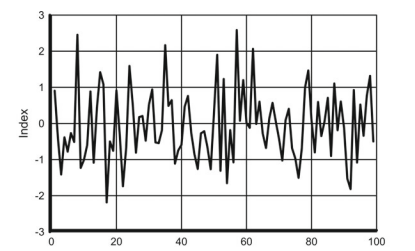
Consider several characteristic examples of climatic or other geophysical processes represented here with short ( $N=100)$ simulated dimensionless time series.
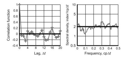
The random processes of a white noise type (Fig. 2.3) are quite common and may include atmospheric pressure, precipitation, and climate indices, for example, the North Atlantic Oscillation. As seen from the figure, the estimates obtained from sample records of white noise do not coincide with the true values of the correlation function and spectral density. This happens due to the sampling variability phenomenon, which occurs whenever the length of the time series that is being analyzed is finite, that is, always. The confidence intervals for the estimated functions in this and other figures in this chapter are not shown intentionally to illustrate the phenomenon of sampling variability.
Another process often encountered in climate and geophysical data in general is the Markov chain, that is, a discrete random process whose future state is independent of its past under the condition that the state of the process at the current time is known. The correlation function of a Gaussian Markov process is defined by its first value $r_{1} \equiv r(1):$
$$
r(k)=r_{1}^{|k|}
$$
The correlation function and spectrum of a Markov process with a positive coefficient $r_{1}$ decrease monotonically as shown in Fig. 2.4. This Markov model is common for many climatic time series. Typical examples are the annual river streamflow and sea level variations. In $1976, \mathrm{~K}$. Hasselmann suggested that the behavior of the climate system can be described with a Markov process (also see Dobrovolski 2000).
A Markov model is often used in climatology to determine statistical reliability of peaks in spectral estimates calculated from time series of geophysical observations. This approach is erroneous because it can only show whether the time series can be regarded as belonging to a Markov process.
Theoretically, the value of $r_{\mathrm{I}}$ can be negative; then, the correlation function will be changing its sign at each lag and the spectrum will be growing with frequency. However, such processes (example b in Fig. 2.2) do not seem to exist in geophysical phenomena.
时间序列分析代考
统计代写|时间序列分析代写Time-Series Analysis代考|Covariance and Correlation Functions
与随机变量相比,随机函数(时间序列)是时间相关的,因此,它们在时域中的属性需要用反映时间序列对时间依赖性的统计矩来描述。通过对时间序列值的乘积进行平均得到的这种混合统计矩
彼此隔开ķ时间间隔是协方差函数R(ķ) :
R(ķ)=林ñ→∞1(ñ−ķ)∑吨=1ñ−ķ(X吨−X¯)(X吨+ķ−X¯),ķ=1,2,…,ķ
除以时间序列方差σX2,它产生相关函数r(ķ)表示时间序列值之间的一系列相关系数X吨和X吨+ķ由ķ时间间隔:
r(ķ)=R(ķ)/σX2.
协方差和相关函数是参数的偶函数ķ以便R(ķ)=R(−ķ)和r(ķ)=r(−ķ). 协方差函数的维度是时间序列维度的平方;如果时间序列以开尔文 (K) 为单位测量,则协方差函数的维度为ķ2. 相关函数是无量纲的。
在下文中,将假设本书中所有时间序列的平均值为零(X¯=0). 此规则的例外情况包括方程式。(4.1) 和 (4.2) 中的平稳性检验。4 ,以及第 1 章中的外推示例。6.
统计代写|时间序列分析代写Time-Series Analysis代考|Spectral Density
标量时间序列最基本的统计特征是它的谱密度s(F); 它定义了时间序列变化的能量如何随频率变化F(每单位时间的周期数),即它在频域中的变化方式。定义谱密度(也称为谱)有多种方法,其中一种是将平稳随机过程的谱密度表示为协方差函数的傅里叶变换:
s(F)=∑ķ=−∞∞R(ķ)和−一世2圆周率ķFΔ吨
在哪里一世=−1和F是从定义的循环频率F=0通过奈奎斯特频率Fñ=1/2Δ吨. 如果Δ吨=1年,频率以每年的周期数 (cpy) 或年为单位测量−1.
协方差函数可以表示为谱密度的傅里叶逆变换:
R(ķ)=∫−FñFñs(F)和一世2圆周率ķFΔ吨 dF
根据方程式。(2.11),谱密度维度是时间序列维度的平方除以频率。因此,如果X吨以毫米为单位测量,频率以每年的周期为单位测量,频谱密度的维度为米米2/Cp是, 或者米米2×年。方程(2.10)和(2.11)构成离散随机过程的 Wiener-Khinchin 定理。论据ķ=0,±1,…协方差函数是离散的,而谱密度是频率的连续函数F. 随机变量(随机向量)的集合不存在协方差和相关函数以及谱密度,因为随机变量不依赖于时间,因此不依赖于频率。
随机过程的一个重要特例是白噪声:一个序列一个吨同分布且相互独立的随机变量。白噪声概念允许引入一类线性规则或规则随机过程,其定义为线性系统(线性滤波器)输出端的过程,输入端有白噪声(Wold 分解):
X吨=∑j=0∞ψj一个吨−j
在哪里ψj是滤波器的系数。通常情况下,假设ψ0=1. 因此,常规随机过程呈现白噪声的线性变换。方程式中总和的上限。(2.12) 可以是有限的,而下限为零,因为如果它小于零,则该过程将在物理上无法实现。如果系数ψj不随时间而改变,如果∑j=0∞|ψj2|<∞, 输出X吨滤波器属于平稳随机过程。数量一个吨也称为创新序列。平均值一个¯方程式中的白噪声。(2.12) 始终为零,因此过程的平均值X吨也是零。本书中的所有时间序列,除潮汐外,都属于有规律的平稳过程。
光谱s(F)正则随机过程是频率的绝对连续函数F,这尤其意味着,规则的随机过程不能表示为有限或可数的无限周期函数集。换句话说,一个规则的随机过程不包含任何谐波。如果假设过程中存在谐波振荡,则过程失去线性规律性,这可能对其分析和预测产生负面影响。但是,如果其频谱包含具有任意窄但有限的频率间隔的尖峰,则该过程保持规则。第 1 章将给出一个例子。4.
统计代写|时间序列分析代写Time-Series Analysis代考|Examples of Geophysical Time Series and Their Statistics
考虑这里用短 (ñ=100)模拟无量纲时间序列。
白噪声类型的随机过程(图 2.3)非常普遍,可能包括大气压力、降水和气候指数,例如北大西洋涛动。从图中可以看出,从白噪声样本记录中得到的估计值与相关函数和谱密度的真实值并不吻合。这是由于采样可变性现象而发生的,只要正在分析的时间序列的长度是有限的,即总是发生,就会发生这种情况。本章中的此图和其他图中的估计函数的置信区间不是为了说明抽样变异现象而有意显示的。
另一个在一般气候和地球物理数据中经常遇到的过程是马尔可夫链,即在当前时间的过程状态已知的条件下,其未来状态与其过去无关的离散随机过程。高斯马尔可夫过程的相关函数由其第一个值定义r1≡r(1):
r(ķ)=r1|ķ|
具有正系数的马尔可夫过程的相关函数和谱r1如图 2.4 所示单调递减。这种马尔可夫模型在许多气候时间序列中很常见。典型的例子是每年的河流流量和海平面变化。在1976, ķ. Hasselmann 建议气候系统的行为可以用马尔可夫过程来描述(另见 Dobrovolski 2000)。
马尔可夫模型通常用于气候学,以确定从地球物理观测的时间序列计算的光谱估计中峰值的统计可靠性。这种方法是错误的,因为它只能表明时间序列是否可以被认为属于马尔可夫过程。
理论上,价值r我可以是负数;然后,相关函数将在每个滞后处改变其符号,并且频谱将随频率增长。然而,这样的过程(图 2.2 中的示例 b)似乎不存在于地球物理现象中。

统计代写请认准statistics-lab™. statistics-lab™为您的留学生涯保驾护航。
金融工程代写
金融工程是使用数学技术来解决金融问题。金融工程使用计算机科学、统计学、经济学和应用数学领域的工具和知识来解决当前的金融问题,以及设计新的和创新的金融产品。
非参数统计代写
非参数统计指的是一种统计方法,其中不假设数据来自于由少数参数决定的规定模型;这种模型的例子包括正态分布模型和线性回归模型。
广义线性模型代考
广义线性模型(GLM)归属统计学领域,是一种应用灵活的线性回归模型。该模型允许因变量的偏差分布有除了正态分布之外的其它分布。
术语 广义线性模型(GLM)通常是指给定连续和/或分类预测因素的连续响应变量的常规线性回归模型。它包括多元线性回归,以及方差分析和方差分析(仅含固定效应)。
有限元方法代写
有限元方法(FEM)是一种流行的方法,用于数值解决工程和数学建模中出现的微分方程。典型的问题领域包括结构分析、传热、流体流动、质量运输和电磁势等传统领域。
有限元是一种通用的数值方法,用于解决两个或三个空间变量的偏微分方程(即一些边界值问题)。为了解决一个问题,有限元将一个大系统细分为更小、更简单的部分,称为有限元。这是通过在空间维度上的特定空间离散化来实现的,它是通过构建对象的网格来实现的:用于求解的数值域,它有有限数量的点。边界值问题的有限元方法表述最终导致一个代数方程组。该方法在域上对未知函数进行逼近。[1] 然后将模拟这些有限元的简单方程组合成一个更大的方程系统,以模拟整个问题。然后,有限元通过变化微积分使相关的误差函数最小化来逼近一个解决方案。
tatistics-lab作为专业的留学生服务机构,多年来已为美国、英国、加拿大、澳洲等留学热门地的学生提供专业的学术服务,包括但不限于Essay代写,Assignment代写,Dissertation代写,Report代写,小组作业代写,Proposal代写,Paper代写,Presentation代写,计算机作业代写,论文修改和润色,网课代做,exam代考等等。写作范围涵盖高中,本科,研究生等海外留学全阶段,辐射金融,经济学,会计学,审计学,管理学等全球99%专业科目。写作团队既有专业英语母语作者,也有海外名校硕博留学生,每位写作老师都拥有过硬的语言能力,专业的学科背景和学术写作经验。我们承诺100%原创,100%专业,100%准时,100%满意。
随机分析代写
随机微积分是数学的一个分支,对随机过程进行操作。它允许为随机过程的积分定义一个关于随机过程的一致的积分理论。这个领域是由日本数学家伊藤清在第二次世界大战期间创建并开始的。
时间序列分析代写
随机过程,是依赖于参数的一组随机变量的全体,参数通常是时间。 随机变量是随机现象的数量表现,其时间序列是一组按照时间发生先后顺序进行排列的数据点序列。通常一组时间序列的时间间隔为一恒定值(如1秒,5分钟,12小时,7天,1年),因此时间序列可以作为离散时间数据进行分析处理。研究时间序列数据的意义在于现实中,往往需要研究某个事物其随时间发展变化的规律。这就需要通过研究该事物过去发展的历史记录,以得到其自身发展的规律。
回归分析代写
多元回归分析渐进(Multiple Regression Analysis Asymptotics)属于计量经济学领域,主要是一种数学上的统计分析方法,可以分析复杂情况下各影响因素的数学关系,在自然科学、社会和经济学等多个领域内应用广泛。
MATLAB代写
MATLAB 是一种用于技术计算的高性能语言。它将计算、可视化和编程集成在一个易于使用的环境中,其中问题和解决方案以熟悉的数学符号表示。典型用途包括:数学和计算算法开发建模、仿真和原型制作数据分析、探索和可视化科学和工程图形应用程序开发,包括图形用户界面构建MATLAB 是一个交互式系统,其基本数据元素是一个不需要维度的数组。这使您可以解决许多技术计算问题,尤其是那些具有矩阵和向量公式的问题,而只需用 C 或 Fortran 等标量非交互式语言编写程序所需的时间的一小部分。MATLAB 名称代表矩阵实验室。MATLAB 最初的编写目的是提供对由 LINPACK 和 EISPACK 项目开发的矩阵软件的轻松访问,这两个项目共同代表了矩阵计算软件的最新技术。MATLAB 经过多年的发展,得到了许多用户的投入。在大学环境中,它是数学、工程和科学入门和高级课程的标准教学工具。在工业领域,MATLAB 是高效研究、开发和分析的首选工具。MATLAB 具有一系列称为工具箱的特定于应用程序的解决方案。对于大多数 MATLAB 用户来说非常重要,工具箱允许您学习和应用专业技术。工具箱是 MATLAB 函数(M 文件)的综合集合,可扩展 MATLAB 环境以解决特定类别的问题。可用工具箱的领域包括信号处理、控制系统、神经网络、模糊逻辑、小波、仿真等。