如果你也在 怎样代写生物统计学Biostatistics这个学科遇到相关的难题,请随时右上角联系我们的24/7代写客服。
生物统计学是将统计技术应用于健康相关领域的科学研究,包括医学、生物学和公共卫生,并开发新的工具来研究这些领域。
statistics-lab™ 为您的留学生涯保驾护航 在代写生物统计学Biostatistics方面已经树立了自己的口碑, 保证靠谱, 高质且原创的统计Statistics代写服务。我们的专家在代写生物统计学Biostatistics方面经验极为丰富,各种代写生物统计学Biostatistics相关的作业也就用不着说。
我们提供的生物统计学Biostatistics及其相关学科的代写,服务范围广, 其中包括但不限于:
- Statistical Inference 统计推断
- Statistical Computing 统计计算
- Advanced Probability Theory 高等楖率论
- Advanced Mathematical Statistics 高等数理统计学
- (Generalized) Linear Models 广义线性模型
- Statistical Machine Learning 统计机器学习
- Longitudinal Data Analysis 纵向数据分析
- Foundations of Data Science 数据科学基础
统计代写|生物统计学作业代写Biostatistics代考|Other Measures of Location
Another useful measure of location is the median. If the observations in the data set are arranged in increasing or decreasing order, the median is the middle observation, which divides the set into equal halves. If the number of observations $n$ is odd, there will be a unique median, the $\frac{1}{2}(n+1)$ th number from either end in the ordered sequence. If $n$ is even, there is strictly no middle observation, but the median is defined by convention as the average of the two middle observations, the $\left(\frac{1}{2} n\right)$ th and $\frac{1}{2}(n+1)$ th from either end. In Section $2.1$ we showed a quicker way to get an approximate value for the median using the cumulative frequency graph (see Figure 2.6).
The two data sets ${8,5,4,12,15,7,28}$ and ${8,5,4,12,15,7,49}$, for example, have different means but the same median, 8 . Therefore, the advantage of the median as a measure of location is that it is less affected by extreme observations. However, the median has some disadvantages in comparison with the mean:
- It takes no account of the precise magnitude of most of the observations and is therefore less efficient than the mean because it wastes information.
- If two groups of observations are pooled, the median of the combined group cannot be expressed in terms of the medians of the two component
NUMERICAL METHODS 77
groups. However, the mean can be so expressed. If component groups are of sizes $n_{1}$ and $n_{2}$ and have means $\bar{x}{1}$ and $\bar{x}{2}$ respectively, the mean of the combined group is
$$
\bar{x}=\frac{n_{1} \bar{x}{1}+n{2} \bar{x}{2}}{n{1}+n_{2}}
$$ - In large data sets, the median requires more work to calculate than the mean and is not much use in the elaborate statistical techniques (it is still useful as a descriptive measure for skewed distributions).
A third measure of location, the mode, was introduced briefly in Section 2.1.3. It is the value at which the frequency polygon reaches a peak. The mode is not used widely in analytical statistics, other than as a descriptive measure, mainly because of the ambiguity in its definition, as the fluctuations of small frequencies are apt to produce spurious modes. For these reasons, in the remainder of the book we focus on a single measure of location, the mean.
统计代写|生物统计学作业代写Biostatistics代考|Measures of Dispersion
When the mean $\bar{x}$ of a set of measurements has been obtained, it is usually a matter of considerable interest to measure the degree of variation or dispersion around this mean. Are the $x$ ‘s all rather close to $\bar{x}$, or are some of them dispersed widely in each direction? This question is important for purely descriptive reasons, but it is also important because the measurement of dispersion or variation plays a central part in the methods of statistical inference described in subsequent chapters.
An obvious candidate for the measurement of dispersion is the range $R$, defined as the difference between the largest value and the smallest value, which was introduced in Section 2.1.3. However, there are a few difficulties about use of the range. The first is that the value of the range is determined by only two of the original observations. Second, the interpretation of the range depends in a complicated way on the number of observations, which is an undesirable feature.
An alternative approach is to make use of deviations from the mean, $x-\bar{x}$; it is obvious that the greater the variation in the data set, the larger the magnitude of these deviations will tend to be. From these deviations, the variance $s^{2}$ is computed by squaring each deviation, adding them, and dividing their sum by one less than $n$ :
$$
s^{2}=\frac{\sum(x-\bar{x})^{2}}{n-1}
$$
The use of the divisor $(n-1)$ instead of $n$ is clearly not very important when $n$ is large. It is more important for small values of $n$, and its justification will be explained briefly later in this section. The following should be noted:
- It would be no use to take the mean of deviations because
$$
\sum(x-\bar{x})=0
$$ - Taking the mean of the absolute values, for example
$$
\frac{\sum|x-\bar{x}|}{n}
$$
is a possibility. However, this measure has the drawback of being difficult to handle mathematically, and we do not consider it further in this book.
The variance $s^{2}$ (s squared) is measured in the square of the units in which the $x^{\prime} s$ are measured. For example, if $x$ is the time in seconds, the variance is measured in seconds squared $\left(\sec ^{2}\right)$. It is convenient, therefore, to have a measure of variation expressed in the same units as the $x$ ‘s, and this can be done easily by taking the square root of the variance. This quantity is the standard deviation, and its formula is
$$
s=\sqrt{\frac{\sum(x-\bar{x})^{2}}{n-1}}
$$
Consider again the data set
$$
{8,5,4,12,15,5,7}
$$
Calculation of the variance $s^{2}$ and standard deviation $s$ is illustrated in Table $2.9$.
统计代写|生物统计学作业代写Biostatistics代考|Box Plots
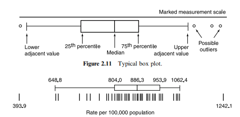
The box plot is a graphical representation of a data set that gives a visual impression of location, spread, and the degree and direction of skewness. It also allows for the identification of outliers. Box plots are similar to one-way scatter plots in that they require a single horizontal axis; however, instead of plotting every observation, they display a summary of the data. A box plot consists of the following:
- A central box extends from the 25 th to the 75 th percentiles. This box is divided into two compartments at the median value of the data set. The relative sizes of the two halves of the box provide an indication of the
Figure 2.12 Crude death rates for the United States, 1988: a combination of one-way scatter and box plots.
distribution symmetry. If they are approximately equal, the data set is roughly symmetric; otherwise, we are able to see the degree and direction of skewness (Figure 2.11).
- The line segments projecting out from the box extend in both directions to the adjacent values. The adjacent values are the points that are $1.5$ times the length of the box beyond either quartile. All other data points outside this range are represented individually by little circles; these are considered to be outliers or extreme observations that are not typical of the rest of the data.
Of course, it is possible to combine a one-way scatter plot and a box plot so as to convey an even greater amount of information (Figure 2.12). There are other ways of constructing box plots; for example, one may make it vertically or divide it into different levels of outliers.
生物统计代写
统计代写|生物统计学作业代写Biostatistics代考|Other Measures of Location
另一个有用的位置度量是中位数。如果数据集中的观测值按升序或降序排列,则中位数是中间观测值,它将集合分成相等的两半。如果观察次数n是奇数,会有一个唯一的中位数,12(n+1)有序序列中任意一端的第 th 个数字。如果n是偶数,严格来说没有中间观测值,但中值按照惯例定义为两个中间观测值的平均值,即(12n)和12(n+1)th 从任一端。在部分2.1我们展示了一种使用累积频率图更快地获得中位数近似值的方法(参见图 2.6)。
两个数据集8,5,4,12,15,7,28和8,5,4,12,15,7,49,例如,具有不同的均值但中位数相同 8 。因此,中位数作为位置度量的优点是受极端观测影响较小。但是,与平均值相比,中位数有一些缺点:
- 它没有考虑大多数观测值的精确幅度,因此效率低于平均值,因为它浪费了信息。
- 如果合并两组观察值,则组合组的中位数不能用两个分量
NUMERICAL METHODS 77
组的中位数来表示。但是,平均值可以这样表达。如果组件组的大小n1和n2并且有意味着 $\bar{x} {1}一种nd\bar{x} {2}r和sp和C吨一世在和l是,吨H和米和一种n这F吨H和C这米b一世n和dGr这在p一世sX¯=n1X¯1+n2X¯2n1+n2$ - 在大型数据集中,中位数需要比平均值更多的工作来计算,并且在复杂的统计技术中用处不大(它仍然可以用作偏态分布的描述性度量)。
第 2.1.3 节简要介绍了第三种位置测量方法,即模式。它是频率多边形达到峰值的值。该模式在分析统计中没有广泛使用,除了作为一种描述性测量,主要是因为它的定义不明确,因为小频率的波动容易产生杂散模式。出于这些原因,在本书的其余部分中,我们将重点放在位置的单一度量上,即均值。
统计代写|生物统计学作业代写Biostatistics代考|Measures of Dispersion
当平均值X¯如果已经获得了一组测量值,那么测量围绕该平均值的变化或离散程度通常是一个相当有趣的问题。是X都相当接近X¯,或者它们中的一些是否广泛分散在各个方向?由于纯粹的描述性原因,这个问题很重要,但也很重要,因为离散度或变异的测量在后续章节中描述的统计推断方法中起着核心作用。
测量色散的一个明显候选者是范围R,定义为最大值与最小值之差,在 2.1.3 节中介绍过。但是,使用该范围存在一些困难。第一个是范围的值仅由两个原始观测值决定。其次,范围的解释以复杂的方式依赖于观察的数量,这是一个不受欢迎的特征。
另一种方法是利用与平均值的偏差,X−X¯; 很明显,数据集的变化越大,这些偏差的幅度就会越大。从这些偏差中,方差s2通过对每个偏差进行平方,将它们相加,然后将它们的总和除以 1 来计算n:
s2=∑(X−X¯)2n−1
除数的使用(n−1)代替n显然不是很重要的时候n很大。对于较小的值更重要n,其理由将在本节后面简要说明。应注意以下几点:
- 取偏差的平均值是没有用的,因为
∑(X−X¯)=0 - 取绝对值的平均值,例如
∑|X−X¯|n
是一种可能。然而,这个度量的缺点是难以用数学方法处理,我们不会在本书中进一步考虑它。
方差s2(s 平方) 以单位的平方来衡量X′s被测量。例如,如果X是以秒为单位的时间,方差以秒的平方为单位测量(秒2). 因此,用与X,这可以通过取方差的平方根来轻松完成。这个量就是标准差,它的公式是
s=∑(X−X¯)2n−1
再次考虑数据集
8,5,4,12,15,5,7
计算方差s2和标准差s如表所示2.9.
统计代写|生物统计学作业代写Biostatistics代考|Box Plots
箱线图是数据集的图形表示,它给出了位置、分布以及偏度的程度和方向的视觉印象。它还允许识别异常值。箱线图类似于单向散点图,因为它们需要一个水平轴;但是,它们不是绘制每个观察值,而是显示数据摘要。箱线图由以下部分组成:
- 一个中心框从第 25 个百分位数延伸到第 75 个百分位数。该框在数据集的中值处分为两个隔间。盒子两半的相对大小提供了一个指示
图 2.12 1988 年美国的粗死亡率:单向散点图和箱线图的组合。
分布对称。如果它们大致相等,则数据集大致对称;否则,我们可以看到偏度的程度和方向(图 2.11)。
- 从框伸出的线段在两个方向上延伸到相邻的值。相邻的值是点1.5超出任一四分位数的盒子长度的倍数。此范围之外的所有其他数据点均由小圆圈单独表示;这些被认为是异常值或极端观察值,它们在其余数据中并不典型。
当然,也可以将单向散点图和箱线图结合起来,以传达更多的信息(图 2.12)。还有其他构建箱线图的方法;例如,可以将其垂直制作或将其划分为不同级别的异常值。

统计代写请认准statistics-lab™. statistics-lab™为您的留学生涯保驾护航。统计代写|python代写代考
随机过程代考
在概率论概念中,随机过程是随机变量的集合。 若一随机系统的样本点是随机函数,则称此函数为样本函数,这一随机系统全部样本函数的集合是一个随机过程。 实际应用中,样本函数的一般定义在时间域或者空间域。 随机过程的实例如股票和汇率的波动、语音信号、视频信号、体温的变化,随机运动如布朗运动、随机徘徊等等。
贝叶斯方法代考
贝叶斯统计概念及数据分析表示使用概率陈述回答有关未知参数的研究问题以及统计范式。后验分布包括关于参数的先验分布,和基于观测数据提供关于参数的信息似然模型。根据选择的先验分布和似然模型,后验分布可以解析或近似,例如,马尔科夫链蒙特卡罗 (MCMC) 方法之一。贝叶斯统计概念及数据分析使用后验分布来形成模型参数的各种摘要,包括点估计,如后验平均值、中位数、百分位数和称为可信区间的区间估计。此外,所有关于模型参数的统计检验都可以表示为基于估计后验分布的概率报表。
广义线性模型代考
广义线性模型(GLM)归属统计学领域,是一种应用灵活的线性回归模型。该模型允许因变量的偏差分布有除了正态分布之外的其它分布。
statistics-lab作为专业的留学生服务机构,多年来已为美国、英国、加拿大、澳洲等留学热门地的学生提供专业的学术服务,包括但不限于Essay代写,Assignment代写,Dissertation代写,Report代写,小组作业代写,Proposal代写,Paper代写,Presentation代写,计算机作业代写,论文修改和润色,网课代做,exam代考等等。写作范围涵盖高中,本科,研究生等海外留学全阶段,辐射金融,经济学,会计学,审计学,管理学等全球99%专业科目。写作团队既有专业英语母语作者,也有海外名校硕博留学生,每位写作老师都拥有过硬的语言能力,专业的学科背景和学术写作经验。我们承诺100%原创,100%专业,100%准时,100%满意。
机器学习代写
随着AI的大潮到来,Machine Learning逐渐成为一个新的学习热点。同时与传统CS相比,Machine Learning在其他领域也有着广泛的应用,因此这门学科成为不仅折磨CS专业同学的“小恶魔”,也是折磨生物、化学、统计等其他学科留学生的“大魔王”。学习Machine learning的一大绊脚石在于使用语言众多,跨学科范围广,所以学习起来尤其困难。但是不管你在学习Machine Learning时遇到任何难题,StudyGate专业导师团队都能为你轻松解决。
多元统计分析代考
基础数据: $N$ 个样本, $P$ 个变量数的单样本,组成的横列的数据表
变量定性: 分类和顺序;变量定量:数值
数学公式的角度分为: 因变量与自变量
时间序列分析代写
随机过程,是依赖于参数的一组随机变量的全体,参数通常是时间。 随机变量是随机现象的数量表现,其时间序列是一组按照时间发生先后顺序进行排列的数据点序列。通常一组时间序列的时间间隔为一恒定值(如1秒,5分钟,12小时,7天,1年),因此时间序列可以作为离散时间数据进行分析处理。研究时间序列数据的意义在于现实中,往往需要研究某个事物其随时间发展变化的规律。这就需要通过研究该事物过去发展的历史记录,以得到其自身发展的规律。
回归分析代写
多元回归分析渐进(Multiple Regression Analysis Asymptotics)属于计量经济学领域,主要是一种数学上的统计分析方法,可以分析复杂情况下各影响因素的数学关系,在自然科学、社会和经济学等多个领域内应用广泛。
MATLAB代写
MATLAB 是一种用于技术计算的高性能语言。它将计算、可视化和编程集成在一个易于使用的环境中,其中问题和解决方案以熟悉的数学符号表示。典型用途包括:数学和计算算法开发建模、仿真和原型制作数据分析、探索和可视化科学和工程图形应用程序开发,包括图形用户界面构建MATLAB 是一个交互式系统,其基本数据元素是一个不需要维度的数组。这使您可以解决许多技术计算问题,尤其是那些具有矩阵和向量公式的问题,而只需用 C 或 Fortran 等标量非交互式语言编写程序所需的时间的一小部分。MATLAB 名称代表矩阵实验室。MATLAB 最初的编写目的是提供对由 LINPACK 和 EISPACK 项目开发的矩阵软件的轻松访问,这两个项目共同代表了矩阵计算软件的最新技术。MATLAB 经过多年的发展,得到了许多用户的投入。在大学环境中,它是数学、工程和科学入门和高级课程的标准教学工具。在工业领域,MATLAB 是高效研究、开发和分析的首选工具。MATLAB 具有一系列称为工具箱的特定于应用程序的解决方案。对于大多数 MATLAB 用户来说非常重要,工具箱允许您学习和应用专业技术。工具箱是 MATLAB 函数(M 文件)的综合集合,可扩展 MATLAB 环境以解决特定类别的问题。可用工具箱的领域包括信号处理、控制系统、神经网络、模糊逻辑、小波、仿真等。