如果你也在 怎样代写金融统计financial statistics这个学科遇到相关的难题,请随时右上角联系我们的24/7代写客服。
金融统计,是将经济物理学应用于金融市场。它没有采用金融学的规范性根基,而是采用实证主义框架。
statistics-lab™ 为您的留学生涯保驾护航 在代写金融统计financial statistics方面已经树立了自己的口碑, 保证靠谱, 高质且原创的统计Statistics代写服务。我们的专家在代写金融统计financial statistics代写方面经验极为丰富,各种代写金融统计financial statistics相关的作业也就用不着说。
我们提供的金融统计financial statistics及其相关学科的代写,服务范围广, 其中包括但不限于:
- Statistical Inference 统计推断
- Statistical Computing 统计计算
- Advanced Probability Theory 高等概率论
- Advanced Mathematical Statistics 高等数理统计学
- (Generalized) Linear Models 广义线性模型
- Statistical Machine Learning 统计机器学习
- Longitudinal Data Analysis 纵向数据分析
- Foundations of Data Science 数据科学基础
统计代写|金融统计代写financial statistics代考|Data description
The empirical experiments are conducted with six stocks and two ETFs. The six individual stocks, which include the Boeing Company (BA), Exxon Mobile Corporation (XOM), Johnson \& Johnson (JNJ), JPMorgan Chase \& Co. (JPM), Microsoft Corporation (MSFT), and Walmart Inc.(WMT), have the highest weight in their corresponding SPDR market sector ETFs such as XLI (industrial sector), XLE (energy sector), XLV (healthcare sector), XLF (finance sector), XLK (technology sector), and XLP (consumer staples sector). The two SPDR sector ETFs chosen are the energy and technology sector ETFs and XLE $\&$ XLK. The dataset is obtained from the Trade and Quote Database (TAQ) of Wharton Research Data Service (WRDS) and it covers the period from January 1, 2006 to December 31, 2013 for a total of 2013 days. We select trade data ranging from 9:30 am to $4 \mathrm{pm}$ on regular trading days. Overnight transactions are excluded from our dataset. We mainly use a 5 -min sampling frequency to eradicate the effect of market microstructure noise in the data which yields 78 total observations per day. We also use a 1-min sampling frequency in specific cases which yields 390 observations per day. It should be noted that all empirical experiments are carried out on the logarithmic values of the stock and ETF prices.
统计代写|金融统计代写financial statistics代考|Methodology
Our empirical experiment consists of three sections: (i) integrated volatility measures, (ii) jump tests, and (iii) co-jump tests. For each of the different parts, we conduct analysis involving the most widely used measures and tests, respectively. A detailed description of the different measures and tests used and the empirical methodologies thereof is given as follows.
First, we use six different measures to estimate Integrated Volatility for all the stocks and ETFs: (1) RV (Section 3.1), (2) BPV (Section 3.2), (3) TPV (Section 3.3), (4) TRV (Section 3.7), (5) MedRV, and (6) MinRV (Section 3.11). Second, to test for price jumps in the data three different jump tests are used: (1) ASJ jump test (Section 4.4), (2) BNS jump test (Section 4.1), and (3) LM jump test (Section 4.2). Lastly, co-jump tests are carried out using (1) JT co-jump test (Section 5.2), (2) BLT co-jump test (Section 5.1), and (3) GST co-exceedance rule (Section 5.4).
Estimation of integrated volatility, BNS and LM jump tests as well as all the co-jump tests are carried out using 5 -min data where $\Delta$ is set to $\frac{1}{78}$. However, for the ASJ jump test, both $1-\left(\Delta=\frac{1}{390}\right)$ and 5 -min frequencies are used as a basis for comparative study.
When conducting analysis using jump tests, we calculate the percentage of days identified as having jumps. For both the BNS and ASJ tests, it can be given as:
Percentage of jump days $=\frac{100 \sum_{i=1}^{T} I\left(Z_{i}>c_{\alpha}\right)}{T} \%$
where $I(\cdot)$ is the jump indicator function, $c_{\alpha}$ is the critical value at $\alpha$ significance level and $Z_{i}$ is the BNS or ASJ jump test statistics. For the LM jump test on the other hand it can be derived as:
$$
\text { Percentage of jump days }=\frac{100 \sum_{i=0}^{T} I\left(\exists t \in i,\left|L_{t}\right|>c_{\alpha}\right)}{T} \%
$$
where $L_{t}$ is the LM jump test statistic at the intra-day level within a particular day, $t$ refers to the 78 intra-day intervals and $c_{\alpha}$ is the critical value at $\alpha$ significance level.
Once jumps are detected, we follow Andersen et al. (2007) and Duong and Swanson (2011) to construct risk measures by separating out the variation due to daily jump component and the continuous components. This is done by using volatility measures $R V$ and $T P V$. It can be given as:
Variation due to jump component $=J V_{t}=\max \left[R V_{t}-T P V_{t}, 0\right] * I_{j u m p, t}$
Consequently the ratio of jump to total variation for all three jump tests can be calculated as:
Ratio of jump variation to total variation $=\frac{J V_{t}}{R V_{t}}$
For BLT co-jump test, the percentage of days identified as having co-jumps is calculated using:
Percentage of co – jump days $=\frac{100 \sum_{i=0}^{T} I\left(\exists j, z_{m c p, i, j}c_{m c p, \alpha, r}\right)}{T} \%$
where $c_{m c p, \alpha, l}$ and $c_{m c p, \alpha, r}$ are left and right tail critical values derived from bootstrapping the null distribution. $\alpha$ is the significance level. For the JT co-jump test, the percentage of days identified as having co-jumps is calculated as:
$$
\text { Percentage of co }-\text { jump days }=\frac{100 \sum_{i-0}^{T} I\left(\Phi_{n}^{(d)} \geq c_{n}^{(d)}\right)}{T} \%
$$
In the co-exceedance rule proposed by Gilder et al. (2014), we use the BNS jump test and the LM jump test to identify co-jumps. The percentage of days identified as having co-jumps can be given as:
Percentage of co -jump days $=\frac{100 \sum_{i=0}^{T} I\left(\left|Z_{i}\right| \geq \Phi_{\alpha}\right) * I\left(\exists t \in i,\left|L_{t}\right|>c_{\alpha}\right)}{T} \%$
where $Z_{i}$ is the BNS jump test statistic and $L_{t}$ is the LM jump test statistic.
In addition to reporting the findings of our empirical experiment on the entire sample, we also conduct analysis after splitting the data set into two periods. The first sample consists of the period from January 2006 to June 2009 and the second sample consists of the period from July 2009 to December 2012. This is done to inspect whether the jump activity in the stocks and the ETFs changes considerably over time. The break date of our sample (June 2009) roughly corresponds to the end of the business cycle contraction after the financial crisis as given by NBER.
统计代写|金融统计代写financial statistics代考|Findings
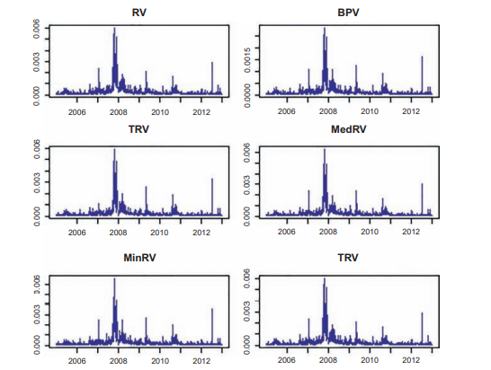
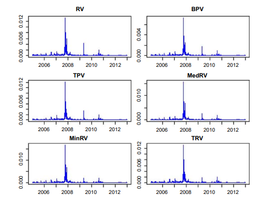
Table 1 gives the summary statistics for integrated volatility which is estimated using six volatility measures $R V, B P V, T P V$, MedRV, MinRV, and $T R V$. The sample period considered for the six stocks and the two ETFs is January 2006-December 2013 . The mean, standard deviation, minimum, and maximum values are all in terms of $10^{-4}$. Among all the stocks and ETFs, JPMorgan seems to have undergone maximum price fluctuations across the sample period as it displays the highest mean and max values across all the volatility measures. On the other hand Johnson \& Johnson and XLK appear to be tied in terms of having undergone least amount of price fluctuations as they display the lowest mean and max volatility estimates. Among all the volatility measures, $B P V$ reports the lowest mean volatility estimate while $R V$ reports the highest mean volatility estimate for any given stock or ETF. This can be explained by the fact that in the presence of frequent jumps, $R V$ overestimates integrated volatility. To get a clearer idea of how volatility differs across the stocks and ETFs, we turn to Figs. 1 and 2 which display the estimated volatility for the stocks Boeing and Exxon with respect to the six aforementioned volatility measures. Similar figures for four other stocks and two ETFs have not been given for the purpose of brevity and can be provided upon request. In general stocks and ETFs achieve their highest volatility in the
fourth quarter of 2008 during the financial crisis with a few exceptions. For XLE, in case of all four volatility measures apart from $T P V$ and $T R V$, volatility reaches its peak in the second quarter of 2009. For XLK on the other hand, only in case $R V$ the volatility peak is reached in the first quarter of 2008 while for the other measures it is the fourth quarter of 2008 .
We now look at Tables $2-5$ which display the descriptive statistics of the three jump tests. For the ASJ jump test we consider both 5- and 1-min frequencies while for the BNS and the LM jump tests we only consider 5 -min frequency. Panel A in the tables refers to the prefinancial crisis sample period, January 2006-June 2009 and panel B refers to the postcrisis period July 2009December 2012. In case of the ASJ jump tests, we find noticeable differences between 5- (Table 2) and 1-min (Table 3) frequencies. Overall the mean value of the statistics is higher for the 1-min data compared to the $5-\mathrm{min}$ frequency suggesting that more jumps would be identified in the 1-min case. The skewness values are all negative irrespective of the sample period, type of stock and frequency of sampling suggesting that the ASJ test statistics are leftskewed. Panel A for both frequencies appear to have overall higher mean and max values again suggesting more jump activity in the financial crises period.
金融统计代写
统计代写|金融统计代写financial statistics代考|Data description
实证实验是用六只股票和两只 ETF 进行的。这六只个股包括波音公司(BA)、埃克森移动公司(XOM)、强生公司(JNJ)、摩根大通公司(JPM)、微软公司(MSFT)和沃尔玛公司( WMT),在其相应的 SPDR 市场板块 ETF 中权重最高,例如 XLI(工业板块)、XLE(能源板块)、XLV(医疗保健板块)、XLF(金融板块)、XLK(科技板块)和 XLP(消费板块)主食部门)。选择的两个 SPDR 行业 ETF 是能源和技术行业 ETF 和 XLE&XLK。该数据集来自沃顿研究数据服务公司(WRDS)的贸易和报价数据库(TAQ),涵盖了从 2006 年 1 月 1 日到 2013 年 12 月 31 日的时间段,共计 2013 天。我们选择从上午 9:30 到4p米在正常交易日。隔夜交易不包括在我们的数据集中。我们主要使用 5 分钟的采样频率来消除数据中市场微观结构噪声的影响,每天总共产生 78 次观察。我们还在特定情况下使用 1 分钟的采样频率,每天产生 390 次观察。需要注意的是,所有的实证实验都是在股票和 ETF 价格的对数值上进行的。
统计代写|金融统计代写financial statistics代考|Methodology
我们的实证实验包括三个部分:(i)综合波动率测量,(ii)跳跃测试,和(iii)共同跳跃测试。对于每个不同的部分,我们分别进行了涉及最广泛使用的测量和测试的分析。下面给出了对所使用的不同测量和测试及其经验方法的详细描述。
首先,我们使用六种不同的方法来估计所有股票和 ETF 的综合波动率:(1) RV(第 3.1 节),(2)BPV(第 3.2 节),(3)TPV(第 3.3 节),(4)TRV(第 3.7 节)、(5) MedRV 和 (6) MinRV(第 3.11 节)。其次,为了测试数据中的价格跳跃,使用了三种不同的跳跃测试:(1)ASJ 跳跃测试(第 4.4 节),(2)BNS 跳跃测试(第 4.1 节)和(3)LM 跳跃测试(第 4.2 节) . 最后,使用 (1) JT 同跳测试(第 5.2 节)、(2) BLT 同跳测试(第 5.1 节)和 (3) GST 共超越规则(第 5.4 节)进行同跳测试。
使用 5 分钟数据进行综合波动率、BNS 和 LM 跳跃测试以及所有共跳测试的估计,其中Δ设定为178. 然而,对于 ASJ 跳跃测试,两者1−(Δ=1390)和 5 分钟频率用作比较研究的基础。
在使用跳跃测试进行分析时,我们会计算被确定为跳跃的天数的百分比。对于 BNS 和 ASJ 测试,它可以给出为:
跳跃天数百分比=100∑一世=1吨一世(从一世>C一种)吨%
在哪里一世(⋅)是跳跃指标函数,C一种是临界值一种显着性水平和从一世是 BNS 或 ASJ 跳跃测试统计。另一方面,对于 LM 跳跃测试,它可以推导出为:
跳跃天数百分比 =100∑一世=0吨一世(∃吨∈一世,|大号吨|>C一种)吨%
在哪里大号吨是特定日期内日内水平的 LM 跳跃测试统计量,吨指 78 个日内间隔和C一种是临界值一种显着性水平。
一旦检测到跳跃,我们就会跟随 Andersen 等人。(2007 年)和 Duong 和 Swanson(2011 年)通过分离每日跳跃分量和连续分量引起的变化来构建风险度量。这是通过使用波动率措施来完成的R在和吨磷在. 可以这样给出:
跳跃成分引起的变化=Ĵ在吨=最大限度[R在吨−吨磷在吨,0]∗一世j在米p,吨
因此,所有三个跳跃测试的跳跃与总变化的比率可以计算为:
跳跃变化与总变化的比率=Ĵ在吨R在吨
对于 BLT 同跳测试,被确定为同跳的天数百分比使用以下公式计算:
共跳天数百分比=100∑一世=0吨一世(∃j,和米Cp,一世,jC米Cp,一种,r)吨%
在哪里C米Cp,一种,l和C米Cp,一种,r是从引导零分布导出的左右尾临界值。一种是显着性水平。对于 JT 同跳测试,被确定为同跳的天数百分比计算如下:
百分比 − 跳天 =100∑一世−0吨一世(披n(d)≥Cn(d))吨%
在 Gilder 等人提出的共同超越规则中。(2014),我们使用 BNS 跳跃测试和 LM 跳跃测试来识别共同跳跃。被确定为有共同跳跃的天数百分比可以表示为:
同跳天数百分比=100∑一世=0吨一世(|从一世|≥披一种)∗一世(∃吨∈一世,|大号吨|>C一种)吨%
在哪里从一世是 BNS 跳跃测试统计量和大号吨是 LM 跳跃检验统计量。
除了报告我们对整个样本的实证实验结果外,我们还将数据集分成两个时期后进行分析。第一个样本包含 2006 年 1 月至 2009 年 6 月期间,第二个样本包含 2009 年 7 月至 2012 年 12 月期间。这样做是为了检查股票和 ETF 的跳跃活动是否随时间发生显着变化。我们样本的中断日期(2009 年 6 月)大致对应于 NBER 给出的金融危机后商业周期收缩的结束。
统计代写|金融统计代写financial statistics代考|Findings
表 1 给出了综合波动率的汇总统计数据,该统计数据使用六种波动率指标进行估计R在,乙磷在,吨磷在、MedRV、MinRV 和吨R在. 六只股票和两只 ETF 的样本期为 2006 年 1 月至 2013 年 12 月。均值、标准差、最小值和最大值均以10−4. 在所有股票和 ETF 中,摩根大通似乎在整个样本期间经历了最大的价格波动,因为它在所有波动性指标中显示出最高的平均值和最大值。另一方面,Johnson \& Johnson 和 XLK 似乎在经历了最少的价格波动方面并列,因为它们显示出最低的平均和最大波动率估计。在所有波动性指标中,乙磷在报告最低的平均波动率估计,而R在报告任何给定股票或 ETF 的最高平均波动率估计。这可以通过以下事实来解释:在频繁跳跃的情况下,R在高估综合波动率。为了更清楚地了解股票和 ETF 之间的波动性有何不同,我们转向图 1。图 1 和 2 显示了波音和埃克森美孚股票相对于上述六种波动率指标的估计波动率。为简洁起见,未提供其他四只股票和两只 ETF 的类似数据,可应要求提供。一般而言,股票和 ETF 在
2008 年第四季度在金融危机期间,除了少数例外。对于 XLE,在所有四种波动性措施的情况下,除了吨磷在和吨R在,波动性在 2009 年第二季度达到顶峰。另一方面,对于 XLK,只有以防万一R在波动性峰值在 2008 年第一季度达到,而其他指标则是在 2008 年第四季度。
我们现在看一下表格2−5它显示了三个跳跃测试的描述性统计数据。对于 ASJ 跳跃测试,我们考虑 5 分钟和 1 分钟频率,而对于 BNS 和 LM 跳跃测试,我们只考虑 5 分钟频率。表中的面板 A 指的是金融危机前的样本期,即 2006 年 1 月至 2009 年 6 月,面板 B 指的是 2009 年 7 月至 2012 年 12 月的危机后时期。在 ASJ 跳跃测试的情况下,我们发现 5-(表 2)和1 分钟(表 3)频率。总体而言,与 1 分钟数据相比,统计数据的平均值更高5−米一世n频率表明在 1 分钟的情况下会发现更多的跳跃。无论样本周期、股票类型和抽样频率如何,偏度值都是负数,这表明 ASJ 测试统计数据是左偏的。两个频率的面板 A 似乎总体上具有更高的平均值和最大值,这再次表明金融危机期间有更多的跳跃活动。

统计代写请认准statistics-lab™. statistics-lab™为您的留学生涯保驾护航。
金融工程代写
金融工程是使用数学技术来解决金融问题。金融工程使用计算机科学、统计学、经济学和应用数学领域的工具和知识来解决当前的金融问题,以及设计新的和创新的金融产品。
非参数统计代写
非参数统计指的是一种统计方法,其中不假设数据来自于由少数参数决定的规定模型;这种模型的例子包括正态分布模型和线性回归模型。
广义线性模型代考
广义线性模型(GLM)归属统计学领域,是一种应用灵活的线性回归模型。该模型允许因变量的偏差分布有除了正态分布之外的其它分布。
术语 广义线性模型(GLM)通常是指给定连续和/或分类预测因素的连续响应变量的常规线性回归模型。它包括多元线性回归,以及方差分析和方差分析(仅含固定效应)。
有限元方法代写
有限元方法(FEM)是一种流行的方法,用于数值解决工程和数学建模中出现的微分方程。典型的问题领域包括结构分析、传热、流体流动、质量运输和电磁势等传统领域。
有限元是一种通用的数值方法,用于解决两个或三个空间变量的偏微分方程(即一些边界值问题)。为了解决一个问题,有限元将一个大系统细分为更小、更简单的部分,称为有限元。这是通过在空间维度上的特定空间离散化来实现的,它是通过构建对象的网格来实现的:用于求解的数值域,它有有限数量的点。边界值问题的有限元方法表述最终导致一个代数方程组。该方法在域上对未知函数进行逼近。[1] 然后将模拟这些有限元的简单方程组合成一个更大的方程系统,以模拟整个问题。然后,有限元通过变化微积分使相关的误差函数最小化来逼近一个解决方案。
tatistics-lab作为专业的留学生服务机构,多年来已为美国、英国、加拿大、澳洲等留学热门地的学生提供专业的学术服务,包括但不限于Essay代写,Assignment代写,Dissertation代写,Report代写,小组作业代写,Proposal代写,Paper代写,Presentation代写,计算机作业代写,论文修改和润色,网课代做,exam代考等等。写作范围涵盖高中,本科,研究生等海外留学全阶段,辐射金融,经济学,会计学,审计学,管理学等全球99%专业科目。写作团队既有专业英语母语作者,也有海外名校硕博留学生,每位写作老师都拥有过硬的语言能力,专业的学科背景和学术写作经验。我们承诺100%原创,100%专业,100%准时,100%满意。
随机分析代写
随机微积分是数学的一个分支,对随机过程进行操作。它允许为随机过程的积分定义一个关于随机过程的一致的积分理论。这个领域是由日本数学家伊藤清在第二次世界大战期间创建并开始的。
时间序列分析代写
随机过程,是依赖于参数的一组随机变量的全体,参数通常是时间。 随机变量是随机现象的数量表现,其时间序列是一组按照时间发生先后顺序进行排列的数据点序列。通常一组时间序列的时间间隔为一恒定值(如1秒,5分钟,12小时,7天,1年),因此时间序列可以作为离散时间数据进行分析处理。研究时间序列数据的意义在于现实中,往往需要研究某个事物其随时间发展变化的规律。这就需要通过研究该事物过去发展的历史记录,以得到其自身发展的规律。
回归分析代写
多元回归分析渐进(Multiple Regression Analysis Asymptotics)属于计量经济学领域,主要是一种数学上的统计分析方法,可以分析复杂情况下各影响因素的数学关系,在自然科学、社会和经济学等多个领域内应用广泛。
MATLAB代写
MATLAB 是一种用于技术计算的高性能语言。它将计算、可视化和编程集成在一个易于使用的环境中,其中问题和解决方案以熟悉的数学符号表示。典型用途包括:数学和计算算法开发建模、仿真和原型制作数据分析、探索和可视化科学和工程图形应用程序开发,包括图形用户界面构建MATLAB 是一个交互式系统,其基本数据元素是一个不需要维度的数组。这使您可以解决许多技术计算问题,尤其是那些具有矩阵和向量公式的问题,而只需用 C 或 Fortran 等标量非交互式语言编写程序所需的时间的一小部分。MATLAB 名称代表矩阵实验室。MATLAB 最初的编写目的是提供对由 LINPACK 和 EISPACK 项目开发的矩阵软件的轻松访问,这两个项目共同代表了矩阵计算软件的最新技术。MATLAB 经过多年的发展,得到了许多用户的投入。在大学环境中,它是数学、工程和科学入门和高级课程的标准教学工具。在工业领域,MATLAB 是高效研究、开发和分析的首选工具。MATLAB 具有一系列称为工具箱的特定于应用程序的解决方案。对于大多数 MATLAB 用户来说非常重要,工具箱允许您学习和应用专业技术。工具箱是 MATLAB 函数(M 文件)的综合集合,可扩展 MATLAB 环境以解决特定类别的问题。可用工具箱的领域包括信号处理、控制系统、神经网络、模糊逻辑、小波、仿真等。