如果你也在 怎样代写金融统计financial statistics这个学科遇到相关的难题，请随时右上角联系我们的24/7代写客服。

金融统计，是将经济物理学应用于金融市场。它没有采用金融学的规范性根基，而是采用实证主义框架。

statistics-lab™ 为您的留学生涯保驾护航 在代写金融统计financial statistics方面已经树立了自己的口碑, 保证靠谱, 高质且原创的统计Statistics代写服务。我们的专家在代写金融统计financial statistics代写方面经验极为丰富，各种代写金融统计financial statistics相关的作业也就用不着说。

我们提供的金融统计financial statistics及其相关学科的代写，服务范围广, 其中包括但不限于:

• Statistical Inference 统计推断
• Statistical Computing 统计计算
• Advanced Probability Theory 高等概率论
• Advanced Mathematical Statistics 高等数理统计学
• (Generalized) Linear Models 广义线性模型
• Statistical Machine Learning 统计机器学习
• Longitudinal Data Analysis 纵向数据分析
• Foundations of Data Science 数据科学基础

统计代写|金融统计代写financial statistics代考|The Augmented Dickey–Fuller test

It is well known in the unit root literature that the limit distribution of the ADF statistic depends on both the null hypothesis and the precise regression model specification. ${ }^{c}$ Appropriate choices of both therefore have a material impact in practical implementation.

The null hypothesis $\left(H_{0}\right)$ of the PSY test captures normal market behaviors and states that asset prices follow a martingale process with a mild drift function such that (Phillips et al., 2014)
$$
y_{t}=g_{T}+y_{t-1}+u_{t},
$$
where $g_{T}=k T^{-\gamma}$ (with constant $k, \gamma>1 / 2$, and sample size $T$ ) captures any mild drift that may be present in prices but which is of smaller order than the martingale component and is therefore asymptotically negligible.
The regression model chosen for the PSY procedure is
$$
\Delta y_{t}=\mu+\rho y_{t-1}+\sum_{j=1}^{p} \phi_{j} \Delta y_{t-j}+v_{t},
$$

where for implementation purposes the regression error $v_{t}$ is assumed to satisfy $v_{t}^{i . i . d} \sim\left(0, \sigma^{2}\right)$. The $p$ lag terms of $\Delta y_{t}$ are included to take care of potential serial correlation. The lag order $p$ is often selected by information criteria. The regression model includes an intercept but no time trend and nests the null hypothesis as a special case with $\mu=g_{T}$ and $\rho=0$. The ADF statistic is simply the $t$-ratio of the least squares estimate of the coefficient $\rho$.

The i.i.d error condition may be replaced with a martingale difference sequence (mds) condition in (2). More general specifications on the error $u_{t}$ in the generating mechanism (1), such as those in Assumption 1 below, may be employed and are accommodated by allowing the regression lag order $p \rightarrow \infty$ as $T \rightarrow \infty$ in (2). Nonparametric adjustments for serial correlation may also be used, such as those developed in Phillips (1987) and Phillips and Perron (1988).

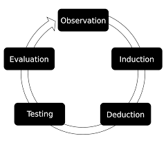
统计代写|金融统计代写financial statistics代考|The Recursive Evolving Algorithm

The recursive evolving algorithm of PSY enables real-time identification of bubbles and crises while allowing for the presence of multiple structural breaks within the sample period. Phillips et al. (2015a,b) show that this algorithm is superior to the forward expanding and rolling window algorithms in bubble identification, especially when the sample period contains multiple bubbles.

For the convenience of exposition, we use the standard “fraction of the total sample” notation for observations. Thus if $t=\lfloor T r\rfloor$ is the integer part of $T r$, then observation $t$ is represented fractionally as observation $r$ and then the total sample runs over values of $r$ from 0 to 1 . Suppose the observation of interest is $r^{\dagger}$. The PSY procedure calculates the ADF statistic recursively from a backward expanding sample sequence. Let $r_{1}$ and $r_{2}$ be the start and end points of the regression sample. The ADF statistic calculated from this sample is denoted by $A D F_{r_{1}}^{r_{2}}$. We fix the end point of all samples on the observation of interest such that $r_{2}=r^{\dagger}$ and allow the start point $r_{1}$ to vary within its feasible range, i.e., $\left[0, r^{\dagger}-r_{0}\right]$, where $r_{0}$ is the minimum window required to initiate the regression. The recommended setting of $r_{0}$ for practical implementation is $r_{0}=0.01$ $+1.8 / \sqrt{T}$. The PSY statistic is the supremum taken over the values of all the ADF statistics in the entire recursion, which is represented mathematically as
$$
P S Y_{r^{\dagger}}\left(r_{0}\right)=\sup {r{1} \in\left[0, r^{\dagger}-r_{0}\right], r_{2}=r^{\dagger}}\left{A D F_{r_{1}}^{r_{2}}\right} .
$$
The supremum enables the selection of the “optimal” starting point of the regression in the sense of providing the largest ADF statistic.

The PSY test can be conducted for each individual observation of interest ranging from $r_{0}$ to 1 , i.e., for $r^{\dagger} \in\left[r_{0}, 1\right]$. The recursive calculation evolves as the observation of interest moves forward and therefore the procedure is called a recursive evolving algorithm. See Fig. 1 for a graphical illustration of the algorithm. The corresponding PSY statistic sequence is $\left{P S Y_{r^{+}}(r 0)\right}_{r^{*} \in[r 0,1]}$.

统计代写|金融统计代写financial statistics代考|The Rationale

To illustrate the idea of bubble identification, consider the present value asset price formula
$$
P_{t}=\sum_{i=0}^{\infty}\left(\frac{1}{1+r_{f}}\right)^{i} \mathbb{E}{t}\left(D{t+i}\right)+B_{t},
$$
where $P_{t}$ is the price of the asset, $D_{t}$ is the payoff received from the asset, $r_{f}$ is the risk-free interest rate, $\mathbb{E}{t}(\cdot)$ is the conditional expectation operator given information to time $t$, and $B{t}$ is the bubble component. The bubble component satisfies the submartingale property (Diba and Grossman, 1988)
$$
\mathbb{E}{t}\left(B{t+1}\right)=\left(1+r_{f}\right) B_{t} .
$$
In the absence of a bubble, the degree of nonstationarity of the asset price is controlled entirely by the dividend series and hence is believed from empirical evidence to be at most $I(1)$. On the other hand, asset prices will be explosive in the presence of a bubble component in formula (7) whenever the initialization $B_{0}>0$ in (8).

Asset price dynamics over the expansionary phase of a bubble period may be modeled in terms of a mildly explosive process (Phillips et al., 2011; Phillips and Magdalinos, 2007; Phillips and Yu, 2009) of the form
$$
\log P_{t}=\delta_{T} \log P_{t-1}+u_{t},
$$
where the autoregressive coefficient $\delta_{T}=1+c T^{-\eta}$ mildly exceeds unity (with $c>0$ and $\eta \in(0,1))$ and yet still lies in its general vicinity. Detection of a bubble process in the data is therefore equivalent to distinguishing a martingale process of asset prices from a mildly explosive process. This can be achieved by the PSY procedure with null and alternative hypotheses specified as
$$
\begin{aligned}
&H_{0}: \mu=g_{T} \text { and } \rho=0, \
&H_{A}: \mu=0 \text { and } \rho>0 .
\end{aligned}
$$

金融统计代写

统计代写|金融统计代写financial statistics代考|The Augmented Dickey–Fuller test

在单位根文献中众所周知，ADF 统计量的极限分布取决于原假设和精确的回归模型规范。CAppropriate choices of both therefore have a material impact in practical implementation.

零假设(H0)的 PSY 测试捕捉正常的市场行为，并指出资产价格遵循具有温和漂移函数的鞅过程，这样 (Phillips et al., 2014)
是吨=G吨+是吨−1+在吨,
在哪里G吨=ķ吨−C（与常数ķ,C>1/2, 和样本量吨) 捕捉价格中可能存在的任何轻微漂移，但其阶次小于鞅分量，因此渐近可忽略不计。
为 PSY 程序选择的回归模型是
Δ是吨=μ+ρ是吨−1+∑j=1pφjΔ是吨−j+在吨,

出于实施目的，回归误差在哪里在吨假设满足在吨一世.一世.d∼(0,σ2). 这p滞后项Δ是吨包括在内以处理潜在的序列相关性。滞后顺序p通常是由信息标准选择的。回归模型包括截距但没有时间趋势，并将原假设嵌套为特殊情况μ=G吨和ρ=0. ADF 统计量就是吨- 系数的最小二乘估计的比率ρ.

iid 错误条件可以替换为 (2) 中的鞅差序列 (mds) 条件。有关错误的更一般规范在吨在生成机制 (1) 中，例如下面的假设 1 中的那些，可以通过允许回归滞后顺序来使用和适应p→∞作为吨→∞在 (2) 中。也可以使用序列相关的非参数调整，例如 Phillips (1987) 和 Phillips and Perron (1988) 开发的那些。

统计代写|金融统计代写financial statistics代考|The Recursive Evolving Algorithm

PSY 的递归演化算法能够实时识别泡沫和危机，同时允许在样本期间存在多个结构中断。菲利普斯等人。（2015a，b）表明该算法在气泡识别方面优于前向扩展和滚动窗口算法，尤其是在样本周期包含多个气泡时。

为方便说明，我们使用标准的“总样本分数”表示法进行观察。因此，如果吨=⌊吨r⌋是整数部分吨r, 然后观察吨分数表示为观察r然后总样本超过r从 0 到 1 。假设感兴趣的观察是r†. PSY 过程从向后扩展的样本序列递归地计算 ADF 统计量。让r1和r2是回归样本的起点和终点。从该样本计算的 ADF 统计量表示为一种DFr1r2. 我们将所有样本的终点固定在感兴趣的观察上，使得r2=r†并允许起点r1在其可行范围内变化，即[0,r†−r0]， 在哪里r0是启动回归所需的最小窗口。推荐的设置r0实际实施是r0=0.01 +1.8/吨. PSY统计量是整个递归过程中所有ADF统计量取值的上确界，数学上表示为
P S Y_{r^{\dagger}}\left(r_{0}\right)=\sup {r{1} \in\left[0, r^{\dagger}-r_{0}\right], r_{2}=r^{\dagger}}\left{A D F_{r_{1}}^{r_{2}}\right} 。P S Y_{r^{\dagger}}\left(r_{0}\right)=\sup {r{1} \in\left[0, r^{\dagger}-r_{0}\right], r_{2}=r^{\dagger}}\left{A D F_{r_{1}}^{r_{2}}\right} 。
在提供最大 ADF 统计量的意义上，上确界能够选择回归的“最佳”起点。

PSY 测试可以针对每个感兴趣的观察进行，范围从r0为 1 ，即，对于r†∈[r0,1]. 递归计算随着感兴趣的观察向前移动而进化，因此该过程称为递归进化算法。有关该算法的图解说明，请参见图 1。对应的 PSY 统计序列为\left{P S Y_{r^{+}}(r 0)\right}_{r^{*} \in[r 0,1]}\left{P S Y_{r^{+}}(r 0)\right}_{r^{*} \in[r 0,1]}.

统计代写|金融统计代写financial statistics代考|The Rationale

为了说明泡沫识别的概念，考虑现值资产价格公式
磷吨=∑一世=0∞(11+rF)一世和吨(D吨+一世)+乙吨,
在哪里磷吨是资产的价格，D吨是从资产中获得的收益，rF是无风险利率，和吨(⋅)是给定时间信息的条件期望算子吨， 和乙吨是气泡成分。气泡成分满足亚鞅性质（Diba 和 Grossman，1988）
和吨(乙吨+1)=(1+rF)乙吨.
在没有泡沫的情况下，资产价格的非平稳程度完全由股利序列控制，因此根据经验证据认为最多为一世(1). 另一方面，每当初始化时，在公式（7）中存在泡沫成分的情况下，资产价格将是爆炸性的乙0>0在 (8) 中。

泡沫时期扩张阶段的资产价格动态可以用以下形式的温和爆炸过程来建模（Phillips 等，2011；Phillips 和 Magdalinos，2007；Phillips 和 Yu，2009）
日志⁡磷吨=d吨日志⁡磷吨−1+在吨,
其中自回归系数d吨=1+C吨−这稍微超过统一（与C>0和这∈(0,1))但仍位于其大体附近。因此，检测数据中的泡沫过程等同于区分资产价格的鞅过程和轻度爆炸过程。这可以通过 PSY 过程来实现，其中零假设和替代假设指定为
H0:μ=G吨 和 ρ=0, H一种:μ=0 和 ρ>0.

统计代写请认准statistics-lab™. statistics-lab™为您的留学生涯保驾护航。

金融工程代写

金融工程是使用数学技术来解决金融问题。金融工程使用计算机科学、统计学、经济学和应用数学领域的工具和知识来解决当前的金融问题，以及设计新的和创新的金融产品。

非参数统计代写

非参数统计指的是一种统计方法，其中不假设数据来自于由少数参数决定的规定模型；这种模型的例子包括正态分布模型和线性回归模型。

广义线性模型代考

广义线性模型（GLM）归属统计学领域，是一种应用灵活的线性回归模型。该模型允许因变量的偏差分布有除了正态分布之外的其它分布。

术语 广义线性模型（GLM）通常是指给定连续和/或分类预测因素的连续响应变量的常规线性回归模型。它包括多元线性回归，以及方差分析和方差分析（仅含固定效应）。

有限元方法代写

有限元方法（FEM）是一种流行的方法，用于数值解决工程和数学建模中出现的微分方程。典型的问题领域包括结构分析、传热、流体流动、质量运输和电磁势等传统领域。

有限元是一种通用的数值方法，用于解决两个或三个空间变量的偏微分方程（即一些边界值问题）。为了解决一个问题，有限元将一个大系统细分为更小、更简单的部分，称为有限元。这是通过在空间维度上的特定空间离散化来实现的，它是通过构建对象的网格来实现的：用于求解的数值域，它有有限数量的点。边界值问题的有限元方法表述最终导致一个代数方程组。该方法在域上对未知函数进行逼近。[1] 然后将模拟这些有限元的简单方程组合成一个更大的方程系统，以模拟整个问题。然后，有限元通过变化微积分使相关的误差函数最小化来逼近一个解决方案。

tatistics-lab作为专业的留学生服务机构，多年来已为美国、英国、加拿大、澳洲等留学热门地的学生提供专业的学术服务，包括但不限于Essay代写，Assignment代写，Dissertation代写，Report代写，小组作业代写，Proposal代写，Paper代写，Presentation代写，计算机作业代写，论文修改和润色，网课代做，exam代考等等。写作范围涵盖高中，本科，研究生等海外留学全阶段，辐射金融，经济学，会计学，审计学，管理学等全球99%专业科目。写作团队既有专业英语母语作者，也有海外名校硕博留学生，每位写作老师都拥有过硬的语言能力，专业的学科背景和学术写作经验。我们承诺100%原创，100%专业，100%准时，100%满意。

随机分析代写

随机微积分是数学的一个分支，对随机过程进行操作。它允许为随机过程的积分定义一个关于随机过程的一致的积分理论。这个领域是由日本数学家伊藤清在第二次世界大战期间创建并开始的。

时间序列分析代写

随机过程，是依赖于参数的一组随机变量的全体，参数通常是时间。 随机变量是随机现象的数量表现，其时间序列是一组按照时间发生先后顺序进行排列的数据点序列。通常一组时间序列的时间间隔为一恒定值（如1秒，5分钟，12小时，7天，1年），因此时间序列可以作为离散时间数据进行分析处理。研究时间序列数据的意义在于现实中，往往需要研究某个事物其随时间发展变化的规律。这就需要通过研究该事物过去发展的历史记录，以得到其自身发展的规律。

回归分析代写

多元回归分析渐进（Multiple Regression Analysis Asymptotics）属于计量经济学领域，主要是一种数学上的统计分析方法，可以分析复杂情况下各影响因素的数学关系，在自然科学、社会和经济学等多个领域内应用广泛。

MATLAB代写

MATLAB 是一种用于技术计算的高性能语言。它将计算、可视化和编程集成在一个易于使用的环境中，其中问题和解决方案以熟悉的数学符号表示。典型用途包括：数学和计算算法开发建模、仿真和原型制作数据分析、探索和可视化科学和工程图形应用程序开发，包括图形用户界面构建MATLAB 是一个交互式系统，其基本数据元素是一个不需要维度的数组。这使您可以解决许多技术计算问题，尤其是那些具有矩阵和向量公式的问题，而只需用 C 或 Fortran 等标量非交互式语言编写程序所需的时间的一小部分。MATLAB 名称代表矩阵实验室。MATLAB 最初的编写目的是提供对由 LINPACK 和 EISPACK 项目开发的矩阵软件的轻松访问，这两个项目共同代表了矩阵计算软件的最新技术。MATLAB 经过多年的发展，得到了许多用户的投入。在大学环境中，它是数学、工程和科学入门和高级课程的标准教学工具。在工业领域，MATLAB 是高效研究、开发和分析的首选工具。MATLAB 具有一系列称为工具箱的特定于应用程序的解决方案。对于大多数 MATLAB 用户来说非常重要，工具箱允许您学习和应用专业技术。工具箱是 MATLAB 函数（M 文件）的综合集合，可扩展 MATLAB 环境以解决特定类别的问题。可用工具箱的领域包括信号处理、控制系统、神经网络、模糊逻辑、小波、仿真等。

R语言代写	问卷设计与分析代写
PYTHON代写	回归分析与线性模型代写
MATLAB代写	方差分析与试验设计代写
STATA代写	机器学习/统计学习代写
SPSS代写	计量经济学代写
EVIEWS代写	时间序列分析代写
EXCEL代写	深度学习代写
SQL代写	各种数据建模与可视化代写

如果你也在 怎样代写金融统计financial statistics这个学科遇到相关的难题，请随时右上角联系我们的24/7代写客服。

金融统计，是将经济物理学应用于金融市场。它没有采用金融学的规范性根基，而是采用实证主义框架。

statistics-lab™ 为您的留学生涯保驾护航 在代写金融统计financial statistics方面已经树立了自己的口碑, 保证靠谱, 高质且原创的统计Statistics代写服务。我们的专家在代写金融统计financial statistics代写方面经验极为丰富，各种代写金融统计financial statistics相关的作业也就用不着说。

我们提供的金融统计financial statistics及其相关学科的代写，服务范围广, 其中包括但不限于:

• Statistical Inference 统计推断
• Statistical Computing 统计计算
• Advanced Probability Theory 高等概率论
• Advanced Mathematical Statistics 高等数理统计学
• (Generalized) Linear Models 广义线性模型
• Statistical Machine Learning 统计机器学习
• Longitudinal Data Analysis 纵向数据分析
• Foundations of Data Science 数据科学基础

统计代写|金融统计代写financial statistics代考|Data description

The empirical experiments are conducted with six stocks and two ETFs. The six individual stocks, which include the Boeing Company (BA), Exxon Mobile Corporation (XOM), Johnson \& Johnson (JNJ), JPMorgan Chase \& Co. (JPM), Microsoft Corporation (MSFT), and Walmart Inc.(WMT), have the highest weight in their corresponding SPDR market sector ETFs such as XLI (industrial sector), XLE (energy sector), XLV (healthcare sector), XLF (finance sector), XLK (technology sector), and XLP (consumer staples sector). The two SPDR sector ETFs chosen are the energy and technology sector ETFs and XLE $\&$ XLK. The dataset is obtained from the Trade and Quote Database (TAQ) of Wharton Research Data Service (WRDS) and it covers the period from January 1, 2006 to December 31, 2013 for a total of 2013 days. We select trade data ranging from 9:30 am to $4 \mathrm{pm}$ on regular trading days. Overnight transactions are excluded from our dataset. We mainly use a 5 -min sampling frequency to eradicate the effect of market microstructure noise in the data which yields 78 total observations per day. We also use a 1-min sampling frequency in specific cases which yields 390 observations per day. It should be noted that all empirical experiments are carried out on the logarithmic values of the stock and ETF prices.

统计代写|金融统计代写financial statistics代考|Methodology

Our empirical experiment consists of three sections: (i) integrated volatility measures, (ii) jump tests, and (iii) co-jump tests. For each of the different parts, we conduct analysis involving the most widely used measures and tests, respectively. A detailed description of the different measures and tests used and the empirical methodologies thereof is given as follows.

First, we use six different measures to estimate Integrated Volatility for all the stocks and ETFs: (1) RV (Section 3.1), (2) BPV (Section 3.2), (3) TPV (Section 3.3), (4) TRV (Section 3.7), (5) MedRV, and (6) MinRV (Section 3.11). Second, to test for price jumps in the data three different jump tests are used: (1) ASJ jump test (Section 4.4), (2) BNS jump test (Section 4.1), and (3) LM jump test (Section 4.2). Lastly, co-jump tests are carried out using (1) JT co-jump test (Section 5.2), (2) BLT co-jump test (Section 5.1), and (3) GST co-exceedance rule (Section 5.4).

Estimation of integrated volatility, BNS and LM jump tests as well as all the co-jump tests are carried out using 5 -min data where $\Delta$ is set to $\frac{1}{78}$. However, for the ASJ jump test, both $1-\left(\Delta=\frac{1}{390}\right)$ and 5 -min frequencies are used as a basis for comparative study.

When conducting analysis using jump tests, we calculate the percentage of days identified as having jumps. For both the BNS and ASJ tests, it can be given as:
Percentage of jump days $=\frac{100 \sum_{i=1}^{T} I\left(Z_{i}>c_{\alpha}\right)}{T} \%$
where $I(\cdot)$ is the jump indicator function, $c_{\alpha}$ is the critical value at $\alpha$ significance level and $Z_{i}$ is the BNS or ASJ jump test statistics. For the LM jump test on the other hand it can be derived as:
$$
\text { Percentage of jump days }=\frac{100 \sum_{i=0}^{T} I\left(\exists t \in i,\left|L_{t}\right|>c_{\alpha}\right)}{T} \%
$$
where $L_{t}$ is the LM jump test statistic at the intra-day level within a particular day, $t$ refers to the 78 intra-day intervals and $c_{\alpha}$ is the critical value at $\alpha$ significance level.

Once jumps are detected, we follow Andersen et al. (2007) and Duong and Swanson (2011) to construct risk measures by separating out the variation due to daily jump component and the continuous components. This is done by using volatility measures $R V$ and $T P V$. It can be given as:

Variation due to jump component $=J V_{t}=\max \left[R V_{t}-T P V_{t}, 0\right] * I_{j u m p, t}$
Consequently the ratio of jump to total variation for all three jump tests can be calculated as:
Ratio of jump variation to total variation $=\frac{J V_{t}}{R V_{t}}$
For BLT co-jump test, the percentage of days identified as having co-jumps is calculated using:

Percentage of co – jump days $=\frac{100 \sum_{i=0}^{T} I\left(\exists j, z_{m c p, i, j}c_{m c p, \alpha, r}\right)}{T} \%$
where $c_{m c p, \alpha, l}$ and $c_{m c p, \alpha, r}$ are left and right tail critical values derived from bootstrapping the null distribution. $\alpha$ is the significance level. For the JT co-jump test, the percentage of days identified as having co-jumps is calculated as:
$$
\text { Percentage of co }-\text { jump days }=\frac{100 \sum_{i-0}^{T} I\left(\Phi_{n}^{(d)} \geq c_{n}^{(d)}\right)}{T} \%
$$
In the co-exceedance rule proposed by Gilder et al. (2014), we use the BNS jump test and the LM jump test to identify co-jumps. The percentage of days identified as having co-jumps can be given as:

Percentage of co -jump days $=\frac{100 \sum_{i=0}^{T} I\left(\left|Z_{i}\right| \geq \Phi_{\alpha}\right) * I\left(\exists t \in i,\left|L_{t}\right|>c_{\alpha}\right)}{T} \%$
where $Z_{i}$ is the BNS jump test statistic and $L_{t}$ is the LM jump test statistic.
In addition to reporting the findings of our empirical experiment on the entire sample, we also conduct analysis after splitting the data set into two periods. The first sample consists of the period from January 2006 to June 2009 and the second sample consists of the period from July 2009 to December 2012. This is done to inspect whether the jump activity in the stocks and the ETFs changes considerably over time. The break date of our sample (June 2009) roughly corresponds to the end of the business cycle contraction after the financial crisis as given by NBER.

统计代写|金融统计代写financial statistics代考|Findings

Table 1 gives the summary statistics for integrated volatility which is estimated using six volatility measures $R V, B P V, T P V$, MedRV, MinRV, and $T R V$. The sample period considered for the six stocks and the two ETFs is January 2006-December 2013 . The mean, standard deviation, minimum, and maximum values are all in terms of $10^{-4}$. Among all the stocks and ETFs, JPMorgan seems to have undergone maximum price fluctuations across the sample period as it displays the highest mean and max values across all the volatility measures. On the other hand Johnson \& Johnson and XLK appear to be tied in terms of having undergone least amount of price fluctuations as they display the lowest mean and max volatility estimates. Among all the volatility measures, $B P V$ reports the lowest mean volatility estimate while $R V$ reports the highest mean volatility estimate for any given stock or ETF. This can be explained by the fact that in the presence of frequent jumps, $R V$ overestimates integrated volatility. To get a clearer idea of how volatility differs across the stocks and ETFs, we turn to Figs. 1 and 2 which display the estimated volatility for the stocks Boeing and Exxon with respect to the six aforementioned volatility measures. Similar figures for four other stocks and two ETFs have not been given for the purpose of brevity and can be provided upon request. In general stocks and ETFs achieve their highest volatility in the

fourth quarter of 2008 during the financial crisis with a few exceptions. For XLE, in case of all four volatility measures apart from $T P V$ and $T R V$, volatility reaches its peak in the second quarter of 2009. For XLK on the other hand, only in case $R V$ the volatility peak is reached in the first quarter of 2008 while for the other measures it is the fourth quarter of 2008 .

We now look at Tables $2-5$ which display the descriptive statistics of the three jump tests. For the ASJ jump test we consider both 5- and 1-min frequencies while for the BNS and the LM jump tests we only consider 5 -min frequency. Panel A in the tables refers to the prefinancial crisis sample period, January 2006-June 2009 and panel B refers to the postcrisis period July 2009December 2012. In case of the ASJ jump tests, we find noticeable differences between 5- (Table 2) and 1-min (Table 3) frequencies. Overall the mean value of the statistics is higher for the 1-min data compared to the $5-\mathrm{min}$ frequency suggesting that more jumps would be identified in the 1-min case. The skewness values are all negative irrespective of the sample period, type of stock and frequency of sampling suggesting that the ASJ test statistics are leftskewed. Panel A for both frequencies appear to have overall higher mean and max values again suggesting more jump activity in the financial crises period.

金融统计代写

统计代写|金融统计代写financial statistics代考|Data description

实证实验是用六只股票和两只 ETF 进行的。这六只个股包括波音公司（BA）、埃克森移动公司（XOM）、强生公司（JNJ）、摩根大通公司（JPM）、微软公司（MSFT）和沃尔玛公司（ WMT)，在其相应的 SPDR 市场板块 ETF 中权重最高，例如 XLI（工业板块）、XLE（能源板块）、XLV（医疗保健板块）、XLF（金融板块）、XLK（科技板块）和 XLP（消费板块）主食部门）。选择的两个 SPDR 行业 ETF 是能源和技术行业 ETF 和 XLE&XLK。该数据集来自沃顿研究数据服务公司（WRDS）的贸易和报价数据库（TAQ），涵盖了从 2006 年 1 月 1 日到 2013 年 12 月 31 日的时间段，共计 2013 天。我们选择从上午 9:30 到4p米在正常交易日。隔夜交易不包括在我们的数据集中。我们主要使用 5 分钟的采样频率来消除数据中市场微观结构噪声的影响，每天总共产生 78 次观察。我们还在特定情况下使用 1 分钟的采样频率，每天产生 390 次观察。需要注意的是，所有的实证实验都是在股票和 ETF 价格的对数值上进行的。

统计代写|金融统计代写financial statistics代考|Methodology

我们的实证实验包括三个部分：（i）综合波动率测量，（ii）跳跃测试，和（iii）共同跳跃测试。对于每个不同的部分，我们分别进行了涉及最广泛使用的测量和测试的分析。下面给出了对所使用的不同测量和测试及其经验方法的详细描述。

首先，我们使用六种不同的方法来估计所有股票和 ETF 的综合波动率：(1) RV（第 3.1 节），（2）BPV（第 3.2 节），（3）TPV（第 3.3 节），（4）TRV（第 3.7 节）、(5) MedRV 和 (6) MinRV（第 3.11 节）。其次，为了测试数据中的价格跳跃，使用了三种不同的跳跃测试：（1）ASJ 跳跃测试（第 4.4 节），（2）BNS 跳跃测试（第 4.1 节）和（3）LM 跳跃测试（第 4.2 节） . 最后，使用 (1) JT 同跳测试（第 5.2 节）、(2) BLT 同跳测试（第 5.1 节）和 (3) GST 共超越规则（第 5.4 节）进行同跳测试。

使用 5 分钟数据进行综合波动率、BNS 和 LM 跳跃测试以及所有共跳测试的估计，其中Δ设定为178. 然而，对于 ASJ 跳跃测试，两者1−(Δ=1390)和 5 分钟频率用作比较研究的基础。

在使用跳跃测试进行分析时，我们会计算被确定为跳跃的天数的百分比。对于 BNS 和 ASJ 测试，它可以给出为：
跳跃天数百分比=100∑一世=1吨一世(从一世>C一种)吨%
在哪里一世(⋅)是跳跃指标函数，C一种是临界值一种显着性水平和从一世是 BNS 或 ASJ 跳跃测试统计。另一方面，对于 LM 跳跃测试，它可以推导出为：
 跳跃天数百分比 =100∑一世=0吨一世(∃吨∈一世,|大号吨|>C一种)吨%
在哪里大号吨是特定日期内日内水平的 LM 跳跃测试统计量，吨指 78 个日内间隔和C一种是临界值一种显着性水平。

一旦检测到跳跃，我们就会跟随 Andersen 等人。（2007 年）和 Duong 和 Swanson（2011 年）通过分离每日跳跃分量和连续分量引起的变化来构建风险度量。这是通过使用波动率措施来完成的R在和吨磷在. 可以这样给出：

跳跃成分引起的变化=Ĵ在吨=最大限度[R在吨−吨磷在吨,0]∗一世j在米p,吨
因此，所有三个跳跃测试的跳跃与总变化的比率可以计算为：
跳跃变化与总变化的比率=Ĵ在吨R在吨
对于 BLT 同跳测试，被确定为同跳的天数百分比使用以下公式计算：

共跳天数百分比=100∑一世=0吨一世(∃j,和米Cp,一世,jC米Cp,一种,r)吨%
在哪里C米Cp,一种,l和C米Cp,一种,r是从引导零分布导出的左右尾临界值。一种是显着性水平。对于 JT 同跳测试，被确定为同跳的天数百分比计算如下：
 百分比 − 跳天 =100∑一世−0吨一世(披n(d)≥Cn(d))吨%
在 Gilder 等人提出的共同超越规则中。（2014），我们使用 BNS 跳跃测试和 LM 跳跃测试来识别共同跳跃。被确定为有共同跳跃的天数百分比可以表示为：

同跳天数百分比=100∑一世=0吨一世(|从一世|≥披一种)∗一世(∃吨∈一世,|大号吨|>C一种)吨%
在哪里从一世是 BNS 跳跃测试统计量和大号吨是 LM 跳跃检验统计量。
除了报告我们对整个样本的实证实验结果外，我们还将数据集分成两个时期后进行分析。第一个样本包含 2006 年 1 月至 2009 年 6 月期间，第二个样本包含 2009 年 7 月至 2012 年 12 月期间。这样做是为了检查股票和 ETF 的跳跃活动是否随时间发生显着变化。我们样本的中断日期（2009 年 6 月）大致对应于 NBER 给出的金融危机后商业周期收缩的结束。

统计代写|金融统计代写financial statistics代考|Findings

表 1 给出了综合波动率的汇总统计数据，该统计数据使用六种波动率指标进行估计R在,乙磷在,吨磷在、MedRV、MinRV 和吨R在. 六只股票和两只 ETF 的样本期为 2006 年 1 月至 2013 年 12 月。均值、标准差、最小值和最大值均以10−4. 在所有股票和 ETF 中，摩根大通似乎在整个样本期间经历了最大的价格波动，因为它在所有波动性指标中显示出最高的平均值和最大值。另一方面，Johnson \& Johnson 和 XLK 似乎在经历了最少的价格波动方面并列，因为它们显示出最低的平均和最大波动率估计。在所有波动性指标中，乙磷在报告最低的平均波动率估计，而R在报告任何给定股票或 ETF 的最高平均波动率估计。这可以通过以下事实来解释：在频繁跳跃的情况下，R在高估综合波动率。为了更清楚地了解股票和 ETF 之间的波动性有何不同，我们转向图 1。图 1 和 2 显示了波音和埃克森美孚股票相对于上述六种波动率指标的估计波动率。为简洁起见，未提供其他四只股票和两只 ETF 的类似数据，可应要求提供。一般而言，股票和 ETF 在

2008 年第四季度在金融危机期间，除了少数例外。对于 XLE，在所有四种波动性措施的情况下，除了吨磷在和吨R在，波动性在 2009 年第二季度达到顶峰。另一方面，对于 XLK，只有以防万一R在波动性峰值在 2008 年第一季度达到，而其他指标则是在 2008 年第四季度。

我们现在看一下表格2−5它显示了三个跳跃测试的描述性统计数据。对于 ASJ 跳跃测试，我们考虑 5 分钟和 1 分钟频率，而对于 BNS 和 LM 跳跃测试，我们只考虑 5 分钟频率。表中的面板 A 指的是金融危机前的样本期，即 2006 年 1 月至 2009 年 6 月，面板 B 指的是 2009 年 7 月至 2012 年 12 月的危机后时期。在 ASJ 跳跃测试的情况下，我们发现 5-（表 2）和1 分钟（表 3）频率。总体而言，与 1 分钟数据相比，统计数据的平均值更高5−米一世n频率表明在 1 分钟的情况下会发现更多的跳跃。无论样本周期、股票类型和抽样频率如何，偏度值都是负数，这表明 ASJ 测试统计数据是左偏的。两个频率的面板 A 似乎总体上具有更高的平均值和最大值，这再次表明金融危机期间有更多的跳跃活动。

统计代写请认准statistics-lab™. statistics-lab™为您的留学生涯保驾护航。

金融工程代写

金融工程是使用数学技术来解决金融问题。金融工程使用计算机科学、统计学、经济学和应用数学领域的工具和知识来解决当前的金融问题，以及设计新的和创新的金融产品。

非参数统计代写

非参数统计指的是一种统计方法，其中不假设数据来自于由少数参数决定的规定模型；这种模型的例子包括正态分布模型和线性回归模型。

广义线性模型代考

广义线性模型（GLM）归属统计学领域，是一种应用灵活的线性回归模型。该模型允许因变量的偏差分布有除了正态分布之外的其它分布。

术语 广义线性模型（GLM）通常是指给定连续和/或分类预测因素的连续响应变量的常规线性回归模型。它包括多元线性回归，以及方差分析和方差分析（仅含固定效应）。

有限元方法代写

有限元方法（FEM）是一种流行的方法，用于数值解决工程和数学建模中出现的微分方程。典型的问题领域包括结构分析、传热、流体流动、质量运输和电磁势等传统领域。

有限元是一种通用的数值方法，用于解决两个或三个空间变量的偏微分方程（即一些边界值问题）。为了解决一个问题，有限元将一个大系统细分为更小、更简单的部分，称为有限元。这是通过在空间维度上的特定空间离散化来实现的，它是通过构建对象的网格来实现的：用于求解的数值域，它有有限数量的点。边界值问题的有限元方法表述最终导致一个代数方程组。该方法在域上对未知函数进行逼近。[1] 然后将模拟这些有限元的简单方程组合成一个更大的方程系统，以模拟整个问题。然后，有限元通过变化微积分使相关的误差函数最小化来逼近一个解决方案。

tatistics-lab作为专业的留学生服务机构，多年来已为美国、英国、加拿大、澳洲等留学热门地的学生提供专业的学术服务，包括但不限于Essay代写，Assignment代写，Dissertation代写，Report代写，小组作业代写，Proposal代写，Paper代写，Presentation代写，计算机作业代写，论文修改和润色，网课代做，exam代考等等。写作范围涵盖高中，本科，研究生等海外留学全阶段，辐射金融，经济学，会计学，审计学，管理学等全球99%专业科目。写作团队既有专业英语母语作者，也有海外名校硕博留学生，每位写作老师都拥有过硬的语言能力，专业的学科背景和学术写作经验。我们承诺100%原创，100%专业，100%准时，100%满意。

随机分析代写

随机微积分是数学的一个分支，对随机过程进行操作。它允许为随机过程的积分定义一个关于随机过程的一致的积分理论。这个领域是由日本数学家伊藤清在第二次世界大战期间创建并开始的。

时间序列分析代写

随机过程，是依赖于参数的一组随机变量的全体，参数通常是时间。 随机变量是随机现象的数量表现，其时间序列是一组按照时间发生先后顺序进行排列的数据点序列。通常一组时间序列的时间间隔为一恒定值（如1秒，5分钟，12小时，7天，1年），因此时间序列可以作为离散时间数据进行分析处理。研究时间序列数据的意义在于现实中，往往需要研究某个事物其随时间发展变化的规律。这就需要通过研究该事物过去发展的历史记录，以得到其自身发展的规律。

回归分析代写

多元回归分析渐进（Multiple Regression Analysis Asymptotics）属于计量经济学领域，主要是一种数学上的统计分析方法，可以分析复杂情况下各影响因素的数学关系，在自然科学、社会和经济学等多个领域内应用广泛。

MATLAB代写

MATLAB 是一种用于技术计算的高性能语言。它将计算、可视化和编程集成在一个易于使用的环境中，其中问题和解决方案以熟悉的数学符号表示。典型用途包括：数学和计算算法开发建模、仿真和原型制作数据分析、探索和可视化科学和工程图形应用程序开发，包括图形用户界面构建MATLAB 是一个交互式系统，其基本数据元素是一个不需要维度的数组。这使您可以解决许多技术计算问题，尤其是那些具有矩阵和向量公式的问题，而只需用 C 或 Fortran 等标量非交互式语言编写程序所需的时间的一小部分。MATLAB 名称代表矩阵实验室。MATLAB 最初的编写目的是提供对由 LINPACK 和 EISPACK 项目开发的矩阵软件的轻松访问，这两个项目共同代表了矩阵计算软件的最新技术。MATLAB 经过多年的发展，得到了许多用户的投入。在大学环境中，它是数学、工程和科学入门和高级课程的标准教学工具。在工业领域，MATLAB 是高效研究、开发和分析的首选工具。MATLAB 具有一系列称为工具箱的特定于应用程序的解决方案。对于大多数 MATLAB 用户来说非常重要，工具箱允许您学习和应用专业技术。工具箱是 MATLAB 函数（M 文件）的综合集合，可扩展 MATLAB 环境以解决特定类别的问题。可用工具箱的领域包括信号处理、控制系统、神经网络、模糊逻辑、小波、仿真等。

R语言代写	问卷设计与分析代写
PYTHON代写	回归分析与线性模型代写
MATLAB代写	方差分析与试验设计代写
STATA代写	机器学习/统计学习代写
SPSS代写	计量经济学代写
EVIEWS代写	时间序列分析代写
EXCEL代写	深度学习代写
SQL代写	各种数据建模与可视化代写

如果你也在 怎样代写金融统计financial statistics这个学科遇到相关的难题，请随时右上角联系我们的24/7代写客服。

金融统计，是将经济物理学应用于金融市场。它没有采用金融学的规范性根基，而是采用实证主义框架。

statistics-lab™ 为您的留学生涯保驾护航 在代写金融统计financial statistics方面已经树立了自己的口碑, 保证靠谱, 高质且原创的统计Statistics代写服务。我们的专家在代写金融统计financial statistics代写方面经验极为丰富，各种代写金融统计financial statistics相关的作业也就用不着说。

我们提供的金融统计financial statistics及其相关学科的代写，服务范围广, 其中包括但不限于:

• Statistical Inference 统计推断
• Statistical Computing 统计计算
• Advanced Probability Theory 高等概率论
• Advanced Mathematical Statistics 高等数理统计学
• (Generalized) Linear Models 广义线性模型
• Statistical Machine Learning 统计机器学习
• Longitudinal Data Analysis 纵向数据分析
• Foundations of Data Science 数据科学基础

统计代写|金融统计代写financial statistics代考|Aı¨t-Sahalia and Jacod test

In Aitt-Sahalia et al. (2009), the authors develop a testing methodology for jumps in the (log) price process by comparing two higher order realized power variations with different sampling intervals, $k \Delta$ and $\Delta$, respectively. In this context $\Delta=\frac{1}{M}, M$ is the number of intra-daily observations and $k$ is a given integer. The $p$ th order realized power variation can be given as
$$
\hat{B}(p, \Delta)=\sum_{j=1}^{M-1}\left|X_{t+(j+1) / M}-X_{t+j / M}\right|^{p}
$$
The ratio of the two realized power variations with different sampling intervals takes the following form
$$
\hat{S}(p, k, \Delta)=\frac{\hat{B}(p, k \Delta)}{\hat{B}(p, \Delta)}
$$
The corresponding jump test statistic can then be defined as:
$$
A S J=\frac{k^{(p / 2)-1}-\hat{S}(p, k, \Delta)}{\sqrt{V_{t, M}}} \stackrel{d}{\rightarrow} N(0,1)
$$
where $V_{t, M}$ can be estimated using either a truncation technique as in
$$
\widehat{V}{t, M}=\Delta \frac{\hat{A}(2 p, \Delta) M(p, k)}{\hat{A}(p, \Delta)^{2}} $$ where $$ \hat{A}(2 p, \Delta)=\frac{\Delta^{1-p / 2}}{\mu{p}} \sum_{j=1}^{M-1}\left|X_{t+(j+1) / M}-X_{t+j / M}\right|^{p} 1_{\left{\left|X_{l+(j+1) / M}-X_{l+j / M}\right| \leq \alpha \Delta^{w}\right}}
$$

or using multipower variation as in
$$
\hat{V}{t, M}=\Delta \frac{M(p, k) \bar{A}(p /([p]+1), 2[p]+2, \Delta)}{\bar{A}(p /([p]+1),[p]+1, \Delta)^{2}} $$ where $$ \begin{gathered} \bar{A}(r, q, \Delta)=\frac{\Delta^{1-q r / 2} M-q+1 q-1}{\mu{r}^{q}} \sum_{j=q} \prod_{i=0}\left|X_{t+(j+i) / M}-X_{t+(j+i-1) / M}\right|^{r}, \
M(p, k)=\frac{1}{\mu_{p}^{2}}\left(k^{p-2}(1+k) \mu_{2 p}+k^{p-2}(k-1) \mu_{p}^{2}-2 k^{p / 2-1}-\mu_{k, p}\right)
\end{gathered}
$$
and $\mu_{r}=E\left(|U|^{r}\right)$ and $\mu_{k, p}=E\left(|U|^{p}\left|U+\sqrt{\left.(k-1) V\right|^{p}}\right|\right)$ for $U, V \sim N(0,1)$. The null hypothesis of no jumps is rejected when the test statistic ASJ is significantly positive.

统计代写|金融统计代写financial statistics代考|Podolskij and Ziggel (PZ) test

In Podolskij and Ziggel $(2010)$ the concept of truncated power variation is used to construct test statistics which diverge to infinity if jumps are present and have a normal distribution otherwise. The jump testing procedure in this chapter is valid (under weak assumptions) for all semimartingales with absolute continuous characteristics and general models for the noise processes. The methodology followed by the authors is a modification of that proposed in Mancini (2009). In particular they consider
$$
T(X, p)=M^{\frac{p-1}{2}} \sum_{j=1}^{M-1}\left|X_{t+(j+1) / M}-X_{t+j / M}\right|^{p}\left(1-\eta_{i} 1_{\left{\left|X_{t+(j+1) / M}-X_{t+j / M}\right| \leq \alpha \Delta^{w}\right}}\right)
$$
where $\left{\eta_{i}\right}_{i \in[1,1 / \Delta]}$ is a sequence of positive i.i.d random variables. The test statistic has the following form
$$
P Z=\frac{T(X, p)}{V a r^{*}(\eta) \hat{A}(2 p, \Delta)} \stackrel{d}{\rightarrow} N(0,1)
$$
where $\hat{A}(2 p, \Delta)$ is the same as in (53).

统计代写|金融统计代写financial statistics代考|Corradi, Silvapulle, and Swanson test

Building on previous work by Aït-Sahalia (2002) and Corradi et al. (2018) design “long time span” jump tests based on realized third moments or “tricity” for the null hypothesis that the probability of a jump is zero. This jump testing methodology is used to detect jumps by examining the “jump intensity” parameter in the data generating process rather than realized jumps over a “fixed time span.” This test is of immense value when one is interested

in using jump diffusion processes for valuation problems like options pricing and default modeling. Let,
$$
\begin{aligned}
\hat{\mu}{3, T, \Delta}=& \frac{1}{T} \sum{j=1}^{n-1}\left(X_{t+(j+1) / M}-X_{t+j / M}-\frac{X_{t+n / M}-X_{t+1 / M}}{n}\right)^{3} \
&-\frac{1}{T^{+}} \sum_{j=1}^{n^{+}-1}\left(X_{t+(j+1) / M}-X_{t+j / M}-\frac{X_{t+n^{+} / M}-X_{t+1 / M}}{n^{+}}\right)^{3} \
& 1\left{\left|X_{t+(j+1) / M}-X_{t+j / M}\right| \leq \tau(\Delta)\right}
\end{aligned}
$$
where we have $n^{+}$observations over an increasing time span of $T^{+}$, a shrinking discrete sampling interval $\Delta=\frac{1}{M}$, so that $n^{+}=\frac{T^{+}}{\Delta}, T^{+} \rightarrow \infty$ and $\Delta \rightarrow 0 . \tau(\Delta)$ is the truncation parameter and one example for the choice of such truncation can be given as follows. If $\sigma_{s}$ as in (1) is a square root process, so that all moments exist, we can set $\tau(\Delta)=c \Delta^{\eta}$ with $\frac{2}{7}<\eta<\frac{1}{2}$. The authors define $n=\frac{T}{\Delta}=n^{+}-\frac{T^{+}-T}{\Delta}$, with $T^{+}>T$ and $\frac{T^{+}}{T} \rightarrow \infty$. Then, the test statistic for the null hypothesis of no jumps can be given as
$$
C S S=\frac{T^{1 / 2}}{\Delta} \hat{\mu}{3, T, \Delta} \stackrel{d}{\rightarrow} N\left(0, \omega{0}\right)
$$
where $\omega_{0}$ is defined in Corradi et al. (2018). Since, under the alternative hypothesis of positive jump intensity, the variance of the statistic is of larger order, it is difficult to construct a variance estimator which is consistent under all hypotheses. The authors use a threshold variance estimator, which removes the contribution of the jump component thus developing an estimator for the variance of Corradi, Silvapulle, and Swanson test $(C S S)$ which is consistent under the null hypothesis of no jumps. Thus we have
$$
\begin{aligned}
\hat{\sigma}{C S S}^{2}=& \frac{1}{\Delta^{2}} \sum{j=0}^{n-1}\left(X_{t+(j+1) / M}-X_{t+j / M}-\frac{X_{t+n / M}-X_{t+1 / M}}{n}\right)^{3} \
& 1\left{\left|X_{t+(j+1) / M}-X_{t+j / M}\right| \leq \tau(\Delta)\right}
\end{aligned}
$$
Thus the $t$-statistic version of the jump test is
$$
t_{C S S}=\frac{C S S}{\hat{\sigma}_{C S S}}
$$

金融统计代写

统计代写|金融统计代写financial statistics代考|Aı¨t-Sahalia and Jacod test

在 Aitt-Sahalia 等人。（2009 年），作者通过比较具有不同采样间隔的两个高阶实现功率变化，开发了一种用于（对数）价格过程中跳跃的测试方法，ķΔ和Δ， 分别。在这种情况下Δ=1米,米是每日内观察的数量和ķ是一个给定的整数。这p三阶实现的功率变化可以给出为
乙^(p,Δ)=∑j=1米−1|X吨+(j+1)/米−X吨+j/米|p
不同采样间隔下两种实现功率变化的比值有如下形式
小号^(p,ķ,Δ)=乙^(p,ķΔ)乙^(p,Δ)
相应的跳跃测试统计量可以定义为：
一种小号Ĵ=ķ(p/2)−1−小号^(p,ķ,Δ)在吨,米→dñ(0,1)
在哪里在吨,米可以使用截断技术来估计，如
在^吨,米=Δ一种^(2p,Δ)米(p,ķ)一种^(p,Δ)2在哪里\hat{A}(2 p, \Delta)=\frac{\Delta^{1-p / 2}}{\mu{p}} \sum_{j=1}^{M-1}\left| X_{t+(j+1) / M}-X_{t+j / M}\right|^{p} 1_{\left{\left|X_{l+(j+1) / M}-X_{l +j / M}\右| \leq \alpha \Delta^{w}\right}}\hat{A}(2 p, \Delta)=\frac{\Delta^{1-p / 2}}{\mu{p}} \sum_{j=1}^{M-1}\left| X_{t+(j+1) / M}-X_{t+j / M}\right|^{p} 1_{\left{\left|X_{l+(j+1) / M}-X_{l +j / M}\右| \leq \alpha \Delta^{w}\right}}

或使用多功率变化，如
在^吨,米=Δ米(p,ķ)一种¯(p/([p]+1),2[p]+2,Δ)一种¯(p/([p]+1),[p]+1,Δ)2在哪里一种¯(r,q,Δ)=Δ1−qr/2米−q+1q−1μrq∑j=q∏一世=0|X吨+(j+一世)/米−X吨+(j+一世−1)/米|r, 米(p,ķ)=1μp2(ķp−2(1+ķ)μ2p+ķp−2(ķ−1)μp2−2ķp/2−1−μķ,p)
和μr=和(|在|r)和μķ,p=和(|在|p|在+(ķ−1)在|p|)为了在,在∼ñ(0,1). 当检验统计量 ASJ 显着为正时，拒绝没有跳跃的原假设。

统计代写|金融统计代写financial statistics代考|Podolskij and Ziggel (PZ) test

在波多尔斯基和齐格尔(2010)截断功率变化的概念用于构建测试统计量，如果存在跳跃则发散到无穷大，否则具有正态分布。本章中的跳跃测试程序对于所有具有绝对连续特征的半鞅和噪声过程的一般模型都是有效的（在弱假设下）。作者采用的方法是对 Mancini (2009) 中提出的方法的修改。他们特别认为
T(X, p)=M^{\frac{p-1}{2}} \sum_{j=1}^{M-1}\left|X_{t+(j+1) / M}-X_ {t+j / M}\right|^{p}\left(1-\eta_{i} 1_{\left{\left|X_{t+(j+1) / M}-X_{t+j / M}\right| \leq \alpha \Delta^{w}\right}}\right)T(X, p)=M^{\frac{p-1}{2}} \sum_{j=1}^{M-1}\left|X_{t+(j+1) / M}-X_ {t+j / M}\right|^{p}\left(1-\eta_{i} 1_{\left{\left|X_{t+(j+1) / M}-X_{t+j / M}\right| \leq \alpha \Delta^{w}\right}}\right)
在哪里\left{\eta_{i}\right}_{i \in[1,1 / \Delta]}\left{\eta_{i}\right}_{i \in[1,1 / \Delta]}是一个正独立同分布随机变量序列。检验统计量具有以下形式
磷从=吨(X,p)在一种r∗(这)一种^(2p,Δ)→dñ(0,1)
在哪里一种^(2p,Δ)与 (53) 相同。

统计代写|金融统计代写financial statistics代考|Corradi, Silvapulle, and Swanson test

基于 Aït-Sahalia (2002) 和 Corradi 等人的先前工作。（2018）基于实现的第三矩或“三度”设计“长时间跨度”跳跃测试，用于跳跃概率为零的零假设。这种跳跃测试方法用于通过检查数据生成过程中的“跳跃强度”参数来检测跳跃，而不是在“固定时间跨度”上实现跳跃。当一个人感兴趣时，这个测试具有巨大的价值

使用跳跃扩散过程解决期权定价和违约建模等估值问题。让，
\begin{aligned} \hat{\mu}{3, T, \Delta}=& \frac{1}{T} \sum{j=1}^{n-1}\left(X_{t+(j +1) / M}-X_{t+j / M}-\frac{X_{t+n / M}-X_{t+1 / M}}{n}\right)^{3} \ &- \frac{1}{T^{+}} \sum_{j=1}^{n^{+}-1}\left(X_{t+(j+1) / M}-X_{t+j / M}-\frac{X_{t+n^{+} / M}-X_{t+1 / M}}{n^{+}}\right)^{3} \ & 1\left{\left |X_{t+(j+1) / M}-X_{t+j / M}\right| \leq \tau(\Delta)\right} \end{对齐}\begin{aligned} \hat{\mu}{3, T, \Delta}=& \frac{1}{T} \sum{j=1}^{n-1}\left(X_{t+(j +1) / M}-X_{t+j / M}-\frac{X_{t+n / M}-X_{t+1 / M}}{n}\right)^{3} \ &- \frac{1}{T^{+}} \sum_{j=1}^{n^{+}-1}\left(X_{t+(j+1) / M}-X_{t+j / M}-\frac{X_{t+n^{+} / M}-X_{t+1 / M}}{n^{+}}\right)^{3} \ & 1\left{\left |X_{t+(j+1) / M}-X_{t+j / M}\right| \leq \tau(\Delta)\right} \end{对齐}
我们在哪里n+在越来越长的时间跨度上的观察吨+, 一个缩小的离散采样间隔Δ=1米， 以便n+=吨+Δ,吨+→∞和Δ→0.τ(Δ)是截断参数，选择这种截断的一个例子如下。如果σs如（1）中是一个平方根过程，所以所有矩都存在，我们可以设置τ(Δ)=CΔ这和27<这<12. 作者定义n=吨Δ=n+−吨+−吨Δ， 和吨+>吨和吨+吨→∞. 然后，没有跳跃的原假设的检验统计量可以给出为
C小号小号=吨1/2Δμ^3,吨,Δ→dñ(0,ω0)
在哪里ω0在 Corradi 等人中定义。（2018 年）。由于在正跳跃强度的备择假设下，统计量的方差具有较大的阶数，因此很难构建在所有假设下都一致的方差估计量。作者使用阈值方差估计器，它消除了跳跃分量的贡献，从而开发了一个用于 Corradi、Silvapulle 和 Swanson 检验的方差的估计器(C小号小号)这在没有跳跃的原假设下是一致的。因此我们有
\begin{对齐} \hat{\sigma}{C S S}^{2}=& \frac{1}{\Delta^{2}} \sum{j=0}^{n-1}\left(X_ {t+(j+1) / M}-X_{t+j / M}-\frac{X_{t+n / M}-X_{t+1 / M}}{n}\right)^{3 } \ & 1\left{\left|X_{t+(j+1) / M}-X_{t+j / M}\right| \leq \tau(\Delta)\right} \end{对齐}\begin{对齐} \hat{\sigma}{C S S}^{2}=& \frac{1}{\Delta^{2}} \sum{j=0}^{n-1}\left(X_ {t+(j+1) / M}-X_{t+j / M}-\frac{X_{t+n / M}-X_{t+1 / M}}{n}\right)^{3 } \ & 1\left{\left|X_{t+(j+1) / M}-X_{t+j / M}\right| \leq \tau(\Delta)\right} \end{对齐}
就这样吨-跳跃测试的统计版本是
吨C小号小号=C小号小号σ^C小号小号

统计代写请认准statistics-lab™. statistics-lab™为您的留学生涯保驾护航。

金融工程代写

金融工程是使用数学技术来解决金融问题。金融工程使用计算机科学、统计学、经济学和应用数学领域的工具和知识来解决当前的金融问题，以及设计新的和创新的金融产品。

非参数统计代写

非参数统计指的是一种统计方法，其中不假设数据来自于由少数参数决定的规定模型；这种模型的例子包括正态分布模型和线性回归模型。

广义线性模型代考

广义线性模型（GLM）归属统计学领域，是一种应用灵活的线性回归模型。该模型允许因变量的偏差分布有除了正态分布之外的其它分布。

术语 广义线性模型（GLM）通常是指给定连续和/或分类预测因素的连续响应变量的常规线性回归模型。它包括多元线性回归，以及方差分析和方差分析（仅含固定效应）。

有限元方法代写

有限元方法（FEM）是一种流行的方法，用于数值解决工程和数学建模中出现的微分方程。典型的问题领域包括结构分析、传热、流体流动、质量运输和电磁势等传统领域。

有限元是一种通用的数值方法，用于解决两个或三个空间变量的偏微分方程（即一些边界值问题）。为了解决一个问题，有限元将一个大系统细分为更小、更简单的部分，称为有限元。这是通过在空间维度上的特定空间离散化来实现的，它是通过构建对象的网格来实现的：用于求解的数值域，它有有限数量的点。边界值问题的有限元方法表述最终导致一个代数方程组。该方法在域上对未知函数进行逼近。[1] 然后将模拟这些有限元的简单方程组合成一个更大的方程系统，以模拟整个问题。然后，有限元通过变化微积分使相关的误差函数最小化来逼近一个解决方案。

tatistics-lab作为专业的留学生服务机构，多年来已为美国、英国、加拿大、澳洲等留学热门地的学生提供专业的学术服务，包括但不限于Essay代写，Assignment代写，Dissertation代写，Report代写，小组作业代写，Proposal代写，Paper代写，Presentation代写，计算机作业代写，论文修改和润色，网课代做，exam代考等等。写作范围涵盖高中，本科，研究生等海外留学全阶段，辐射金融，经济学，会计学，审计学，管理学等全球99%专业科目。写作团队既有专业英语母语作者，也有海外名校硕博留学生，每位写作老师都拥有过硬的语言能力，专业的学科背景和学术写作经验。我们承诺100%原创，100%专业，100%准时，100%满意。

随机分析代写

随机微积分是数学的一个分支，对随机过程进行操作。它允许为随机过程的积分定义一个关于随机过程的一致的积分理论。这个领域是由日本数学家伊藤清在第二次世界大战期间创建并开始的。

时间序列分析代写

随机过程，是依赖于参数的一组随机变量的全体，参数通常是时间。 随机变量是随机现象的数量表现，其时间序列是一组按照时间发生先后顺序进行排列的数据点序列。通常一组时间序列的时间间隔为一恒定值（如1秒，5分钟，12小时，7天，1年），因此时间序列可以作为离散时间数据进行分析处理。研究时间序列数据的意义在于现实中，往往需要研究某个事物其随时间发展变化的规律。这就需要通过研究该事物过去发展的历史记录，以得到其自身发展的规律。

回归分析代写

多元回归分析渐进（Multiple Regression Analysis Asymptotics）属于计量经济学领域，主要是一种数学上的统计分析方法，可以分析复杂情况下各影响因素的数学关系，在自然科学、社会和经济学等多个领域内应用广泛。

MATLAB代写

MATLAB 是一种用于技术计算的高性能语言。它将计算、可视化和编程集成在一个易于使用的环境中，其中问题和解决方案以熟悉的数学符号表示。典型用途包括：数学和计算算法开发建模、仿真和原型制作数据分析、探索和可视化科学和工程图形应用程序开发，包括图形用户界面构建MATLAB 是一个交互式系统，其基本数据元素是一个不需要维度的数组。这使您可以解决许多技术计算问题，尤其是那些具有矩阵和向量公式的问题，而只需用 C 或 Fortran 等标量非交互式语言编写程序所需的时间的一小部分。MATLAB 名称代表矩阵实验室。MATLAB 最初的编写目的是提供对由 LINPACK 和 EISPACK 项目开发的矩阵软件的轻松访问，这两个项目共同代表了矩阵计算软件的最新技术。MATLAB 经过多年的发展，得到了许多用户的投入。在大学环境中，它是数学、工程和科学入门和高级课程的标准教学工具。在工业领域，MATLAB 是高效研究、开发和分析的首选工具。MATLAB 具有一系列称为工具箱的特定于应用程序的解决方案。对于大多数 MATLAB 用户来说非常重要，工具箱允许您学习和应用专业技术。工具箱是 MATLAB 函数（M 文件）的综合集合，可扩展 MATLAB 环境以解决特定类别的问题。可用工具箱的领域包括信号处理、控制系统、神经网络、模糊逻辑、小波、仿真等。

R语言代写	问卷设计与分析代写
PYTHON代写	回归分析与线性模型代写
MATLAB代写	方差分析与试验设计代写
STATA代写	机器学习/统计学习代写
SPSS代写	计量经济学代写
EVIEWS代写	时间序列分析代写
EXCEL代写	深度学习代写
SQL代写	各种数据建模与可视化代写

如果你也在 怎样代写金融统计financial statistics这个学科遇到相关的难题，请随时右上角联系我们的24/7代写客服。

金融统计，是将经济物理学应用于金融市场。它没有采用金融学的规范性根基，而是采用实证主义框架。

statistics-lab™ 为您的留学生涯保驾护航 在代写金融统计financial statistics方面已经树立了自己的口碑, 保证靠谱, 高质且原创的统计Statistics代写服务。我们的专家在代写金融统计financial statistics代写方面经验极为丰富，各种代写金融统计financial statistics相关的作业也就用不着说。

我们提供的金融统计financial statistics及其相关学科的代写，服务范围广, 其中包括但不限于:

• Statistical Inference 统计推断
• Statistical Computing 统计计算
• Advanced Probability Theory 高等概率论
• Advanced Mathematical Statistics 高等数理统计学
• (Generalized) Linear Models 广义线性模型
• Statistical Machine Learning 统计机器学习
• Longitudinal Data Analysis 纵向数据分析
• Foundations of Data Science 数据科学基础

统计代写|金融统计代写financial statistics代考|Barndorff-Nielsen and Shephard test

To test for the existence of jumps in the sample path of asset prices, Barndorff-Nielsen and Shephard (2006) propose nonparametric Hausman (1978) type tests using the difference between Realized Quadratic Variation, an estimator of integrated volatility which is not robust to jumps, and $B P V$, which is a jump robust estimator of integrated volatility. Realized Quadratic Variation is considered to be the same as $R V$. The adjusted jump ratio test statistic can be given as:
$$
B N S=\frac{M^{1 / 2}}{\sqrt{\vartheta \max \left(1, \frac{Q P V}{\left(\mu_{1}^{2} B P V\right)^{2}}\right)}}\left(1-\frac{B P V}{R V}\right) \stackrel{d}{\rightarrow} N(0,1)
$$
where $B P V$ is the same as in $(13), R V$ is the same as in $(12), \theta=\left(\left(\pi^{2} / 4\right)+\right.$ $\pi-5) \approx 0.6090$. The realized quadpower variation $Q P V$ is used to estimate integrated quarticity $\left(\int_{0}^{t} \sigma_{s}^{4} d s\right)$ and can be given as:
$$
Q P V=M \sum_{j=4}^{M}\left|\Delta_{j} X\left|\Delta_{j-1} X\right| \Delta_{j-2} X | \Delta_{j-3} X\right| \stackrel{d}{\rightarrow} \mu_{1}^{4} \int_{0}^{t} \sigma_{s}^{4} d s
$$
The authors show that the null hypothesis of no jumps is rejected if the test statistic Barndorff-Nielsen and Shephard test (BNS) is significantly positive.

统计代写|金融统计代写financial statistics代考|Lee and Mykland test

Lee and Mykland (2007) use the ratio of realized return to estimated instantaneous volatility, and further construct a nonparametric jump test to detect the exact timing of jumps at the intra-day level. The test statistic which identifies whether there is a jump during $(t+j / M, t+(j+1) / M]$ can be given as:
16 PART | I Finance
$$
L_{(t+(j+1) / M)}=\frac{X_{t+(j+1) / M}-X_{t+j / M}}{\sigma_{t+(j+1) / M}}
$$
where
$$
\sigma_{t+\widetilde{(j+1)} / M^{2}} \equiv \frac{1}{K-2} \sum_{i=j-K+1}^{j-2}\left|X_{t+(i+1) / M}-X_{t+i / M}\right|\left|X_{t+i / M}-X_{t+(i-1) / M}\right|
$$
Here $K$ is the window size of a local movement of the process. It is chosen in a way such that the effect of jumps on volatility estimation is eliminated. The authors suggest a value of $K=10$ when the sampling frequency is $5 \mathrm{~min}$. Thus, it can be asymptotically shown that
$$
\frac{\max {j \in \bar{A}{M}}\left|L_{(t+(j+1) / M)}\right|-C_{M}}{S_{M}} \rightarrow \varepsilon, \text { as } \Delta t \rightarrow 0
$$
where $\varepsilon$ has a cumulative distribution function $P(\varepsilon \leq x)=\exp \left(-e^{-x}\right)$,
$$
C_{M}=\frac{(2 \log M)^{1 / 2}}{c}-\frac{\log \pi+\log (\log M)}{2 c(2 \log M)^{1 / 2}} \text { and } s_{M}=\frac{1}{c(2 \log M)^{1 / 2}}
$$
$M$ is the number of intra-daily observations, $c \approx 0.7979$ and $\bar{A}_{M}$ is the set of $j$ $\in{0,1, \ldots, M}$ so that there are no jumps in $(t+j / M, t+(j+1) / M]$.

统计代写|金融统计代写financial statistics代考|Jiang and Oomen test

Jiang and Oomen (2008) compare a jump sensitive variance measure to $R V$ in order to test for jumps. Their idea is based on the fact that in the absence of jumps the accumulated difference between the simple return and log return (called the swap variance) captures one-half of the integrated volatility in the continuous time limit. Consequently it can be stated, in the absence of jumps the difference between swap variance and $R V$ should be zero, while in the presence of jumps the same difference reflects the replication error of variance swap thus detecting jumps. The swap variance can be given as:
$$
S V_{t, M}=2 \sum_{j=1}^{M-1}\left(\Delta_{j} P-\Delta_{j} X\right)
$$
where $Y=\log (P)$ and $Y$ is the same as in (1). $\Delta_{j} P=\frac{P_{f+(i+1) / M}}{P_{t+j / M}}-1$ and $\Delta_{j} X$ is the same as in (10). The three different swap variance tests proposed by the authors can be given as:
(i) The difference test:
$$
\frac{M}{\Omega_{S V}}\left(S V_{t, M}-R V_{t, M}\right) \stackrel{d}{\rightarrow} N(0,1)
$$

(ii) The logarithmic test:
$$
\frac{B P V_{t, M} M}{\Omega_{S V}}\left(\log \left(S V_{t, M}\right)-\log \left(R V_{t, M}\right)\right) \stackrel{d}{\rightarrow} N(0,1)
$$
(iii) The ratio test:
$$
\frac{B P V_{t, M} M}{\Omega_{S V}}\left(1-\frac{R V_{t, M}}{S V_{t, M}}\right) \stackrel{d}{\rightarrow} N(0,1)
$$
where $\Omega_{S V}=\frac{\mu_{6} M^{3} \mu_{6 j p}^{-p}}{9 M-p+1} \sum_{j=1}^{M-p} \prod_{k=0}^{p}\left|\Delta_{j+k} X\right|^{6 / p}$ for $p \in{1,2, \ldots}, \mu_{z}=E\left(|x|^{z}\right)$ for $z \sim N(0,1) .$

金融统计代写

统计代写|金融统计代写financial statistics代考|Barndorff-Nielsen and Shephard test

为了检验资产价格样本路径中是否存在跳跃，Barndorff-Nielsen 和 Shephard (2006) 提出了非参数 Hausman (1978) 类型检验，使用已实现二次变量之间的差异，这是一种对跳跃不具有鲁棒性的综合波动率估计量， 和乙磷在，这是综合波动率的跳跃稳健估计。已实现的二次变分被认为与R在. 调整后的跳跃比检验统计量可以给出为：
乙ñ小号=米1/2ϑ最大限度(1,问磷在(μ12乙磷在)2)(1−乙磷在R在)→dñ(0,1)
在哪里乙磷在与中相同(13),R在与中相同(12),θ=((圆周率2/4)+ 圆周率−5)≈0.6090. 实现的四次幂变化问磷在用于估计积分四分位数(∫0吨σs4ds)并且可以给出为：
问磷在=米∑j=4米|ΔjX|Δj−1X|Δj−2X|Δj−3X|→dμ14∫0吨σs4ds
作者表明，如果检验统计量 Barndorff-Nielsen 和 Shephard 检验 (BNS) 显着阳性，则拒绝没有跳跃的零假设。

统计代写|金融统计代写financial statistics代考|Lee and Mykland test

Lee 和 Mykland (2007) 使用已实现收益与估计瞬时波动率的比率，并进一步构建了非参数跳跃检验来检测当日水平跳跃的确切时间。确定是否有跳跃的检验统计量(吨+j/米,吨+(j+1)/米]可以给出：
16 PART | 我金融
大号(吨+(j+1)/米)=X吨+(j+1)/米−X吨+j/米σ吨+(j+1)/米
在哪里
σ吨+(j+1)~/米2≡1ķ−2∑一世=j−ķ+1j−2|X吨+(一世+1)/米−X吨+一世/米||X吨+一世/米−X吨+(一世−1)/米|
这里ķ是进程局部移动的窗口大小。它的选择方式可以消除跳跃对波动率估计的影响。作者建议价值ķ=10当采样频率为5 米一世n. 因此，可以渐近地证明
最大限度j∈一种¯米|大号(吨+(j+1)/米)|−C米小号米→e, 作为 Δ吨→0
在哪里e具有累积分布函数磷(e≤X)=经验⁡(−和−X),
C米=(2日志⁡米)1/2C−日志⁡圆周率+日志⁡(日志⁡米)2C(2日志⁡米)1/2 和 s米=1C(2日志⁡米)1/2
米是每日内观察的数量，C≈0.7979和一种¯米是集合j ∈0,1,…,米所以没有跳跃(吨+j/米,吨+(j+1)/米].

统计代写|金融统计代写financial statistics代考|Jiang and Oomen test

Jiang 和 Oomen (2008) 将跳跃敏感方差测量与R在为了测试跳跃。他们的想法是基于这样一个事实，即在没有跳跃的情况下，简单收益和对数收益之间的累积差异（称为掉期方差）在连续时间限制内捕获了综合波动率的一半。因此可以说，在没有跳跃的情况下，互换方差和R在应该为零，而在存在跳跃的情况下，相同的差异反映了方差交换的复制误差，从而检测到了跳跃。互换方差可以表示为：
小号在吨,米=2∑j=1米−1(Δj磷−ΔjX)
在哪里是=日志⁡(磷)和是与（1）中的相同。Δj磷=磷F+(一世+1)/米磷吨+j/米−1和ΔjX与（10）中的相同。作者提出的三种不同的掉期方差检验可以如下给出：
(i) 差异检验：
米Ω小号在(小号在吨,米−R在吨,米)→dñ(0,1)

(ii) 对数检验：
乙磷在吨,米米Ω小号在(日志⁡(小号在吨,米)−日志⁡(R在吨,米))→dñ(0,1)
(iii) 比率测试：
乙磷在吨,米米Ω小号在(1−R在吨,米小号在吨,米)→dñ(0,1)
在哪里Ω小号在=μ6米3μ6jp−p9米−p+1∑j=1米−p∏ķ=0p|Δj+ķX|6/p为了p∈1,2,…,μ和=和(|X|和)为了和∼ñ(0,1).

统计代写请认准statistics-lab™. statistics-lab™为您的留学生涯保驾护航。

金融工程代写

金融工程是使用数学技术来解决金融问题。金融工程使用计算机科学、统计学、经济学和应用数学领域的工具和知识来解决当前的金融问题，以及设计新的和创新的金融产品。

非参数统计代写

非参数统计指的是一种统计方法，其中不假设数据来自于由少数参数决定的规定模型；这种模型的例子包括正态分布模型和线性回归模型。

广义线性模型代考

广义线性模型（GLM）归属统计学领域，是一种应用灵活的线性回归模型。该模型允许因变量的偏差分布有除了正态分布之外的其它分布。

术语 广义线性模型（GLM）通常是指给定连续和/或分类预测因素的连续响应变量的常规线性回归模型。它包括多元线性回归，以及方差分析和方差分析（仅含固定效应）。

有限元方法代写

有限元方法（FEM）是一种流行的方法，用于数值解决工程和数学建模中出现的微分方程。典型的问题领域包括结构分析、传热、流体流动、质量运输和电磁势等传统领域。

有限元是一种通用的数值方法，用于解决两个或三个空间变量的偏微分方程（即一些边界值问题）。为了解决一个问题，有限元将一个大系统细分为更小、更简单的部分，称为有限元。这是通过在空间维度上的特定空间离散化来实现的，它是通过构建对象的网格来实现的：用于求解的数值域，它有有限数量的点。边界值问题的有限元方法表述最终导致一个代数方程组。该方法在域上对未知函数进行逼近。[1] 然后将模拟这些有限元的简单方程组合成一个更大的方程系统，以模拟整个问题。然后，有限元通过变化微积分使相关的误差函数最小化来逼近一个解决方案。

tatistics-lab作为专业的留学生服务机构，多年来已为美国、英国、加拿大、澳洲等留学热门地的学生提供专业的学术服务，包括但不限于Essay代写，Assignment代写，Dissertation代写，Report代写，小组作业代写，Proposal代写，Paper代写，Presentation代写，计算机作业代写，论文修改和润色，网课代做，exam代考等等。写作范围涵盖高中，本科，研究生等海外留学全阶段，辐射金融，经济学，会计学，审计学，管理学等全球99%专业科目。写作团队既有专业英语母语作者，也有海外名校硕博留学生，每位写作老师都拥有过硬的语言能力，专业的学科背景和学术写作经验。我们承诺100%原创，100%专业，100%准时，100%满意。

随机分析代写

随机微积分是数学的一个分支，对随机过程进行操作。它允许为随机过程的积分定义一个关于随机过程的一致的积分理论。这个领域是由日本数学家伊藤清在第二次世界大战期间创建并开始的。

时间序列分析代写

随机过程，是依赖于参数的一组随机变量的全体，参数通常是时间。 随机变量是随机现象的数量表现，其时间序列是一组按照时间发生先后顺序进行排列的数据点序列。通常一组时间序列的时间间隔为一恒定值（如1秒，5分钟，12小时，7天，1年），因此时间序列可以作为离散时间数据进行分析处理。研究时间序列数据的意义在于现实中，往往需要研究某个事物其随时间发展变化的规律。这就需要通过研究该事物过去发展的历史记录，以得到其自身发展的规律。

回归分析代写

多元回归分析渐进（Multiple Regression Analysis Asymptotics）属于计量经济学领域，主要是一种数学上的统计分析方法，可以分析复杂情况下各影响因素的数学关系，在自然科学、社会和经济学等多个领域内应用广泛。

MATLAB代写

MATLAB 是一种用于技术计算的高性能语言。它将计算、可视化和编程集成在一个易于使用的环境中，其中问题和解决方案以熟悉的数学符号表示。典型用途包括：数学和计算算法开发建模、仿真和原型制作数据分析、探索和可视化科学和工程图形应用程序开发，包括图形用户界面构建MATLAB 是一个交互式系统，其基本数据元素是一个不需要维度的数组。这使您可以解决许多技术计算问题，尤其是那些具有矩阵和向量公式的问题，而只需用 C 或 Fortran 等标量非交互式语言编写程序所需的时间的一小部分。MATLAB 名称代表矩阵实验室。MATLAB 最初的编写目的是提供对由 LINPACK 和 EISPACK 项目开发的矩阵软件的轻松访问，这两个项目共同代表了矩阵计算软件的最新技术。MATLAB 经过多年的发展，得到了许多用户的投入。在大学环境中，它是数学、工程和科学入门和高级课程的标准教学工具。在工业领域，MATLAB 是高效研究、开发和分析的首选工具。MATLAB 具有一系列称为工具箱的特定于应用程序的解决方案。对于大多数 MATLAB 用户来说非常重要，工具箱允许您学习和应用专业技术。工具箱是 MATLAB 函数（M 文件）的综合集合，可扩展 MATLAB 环境以解决特定类别的问题。可用工具箱的领域包括信号处理、控制系统、神经网络、模糊逻辑、小波、仿真等。

R语言代写	问卷设计与分析代写
PYTHON代写	回归分析与线性模型代写
MATLAB代写	方差分析与试验设计代写
STATA代写	机器学习/统计学习代写
SPSS代写	计量经济学代写
EVIEWS代写	时间序列分析代写
EXCEL代写	深度学习代写
SQL代写	各种数据建模与可视化代写

如果你也在 怎样代写金融统计financial statistics这个学科遇到相关的难题，请随时右上角联系我们的24/7代写客服。

金融统计，是将经济物理学应用于金融市场。它没有采用金融学的规范性根基，而是采用实证主义框架。

statistics-lab™ 为您的留学生涯保驾护航 在代写金融统计financial statistics方面已经树立了自己的口碑, 保证靠谱, 高质且原创的统计Statistics代写服务。我们的专家在代写金融统计financial statistics代写方面经验极为丰富，各种代写金融统计financial statistics相关的作业也就用不着说。

我们提供的金融统计financial statistics及其相关学科的代写，服务范围广, 其中包括但不限于:

• Statistical Inference 统计推断
• Statistical Computing 统计计算
• Advanced Probability Theory 高等概率论
• Advanced Mathematical Statistics 高等数理统计学
• (Generalized) Linear Models 广义线性模型
• Statistical Machine Learning 统计机器学习
• Longitudinal Data Analysis 纵向数据分析
• Foundations of Data Science 数据科学基础

统计代写|金融统计代写financial statistics代考|Multiscale realized volatility

The TSRV estimator is not efficient although it has many desirable properties. The rate of convergence for TSRV is not satisfactory, it converges to the true volatility (IV in the absence of jumps) only at the rate of $M^{-1 / 6}$. The multiscale realized volatility (MSRV) is proposed in Zhang et al. (2006). This is a microstructure noise robust measure which converged to $I V$ (in the absence of jumps) at the rate of $M^{-1 / 4}$. While TSRV uses two time scales, $M S R V$ on the other hand uses $N$ different time scales. $M S R V$ takes the following form
$$
M S R V_{t, M}=\sum_{n=1}^{N} a_{n}[X, X]^{\left(M, K_{n}\right)}, n=1, \ldots, N
$$
where
$$
\begin{array}{r}
a_{n}=12 \frac{n}{N^{2}} \frac{n / N-1 / 2-1 /(2 N)}{1-1 / N^{2}}, \sum_{n=1}^{N} a_{n}=1 \text { and } \sum_{n=1}^{N} a_{n} / n=0 \
{[X, X]^{\left(M, K_{n}\right)}=\frac{1}{K_{n}} \sum_{l=1}^{K_{n}} \sum_{j=1}^{m_{n, l}-1}\left(X_{t+\left((j+1) K_{n}+l\right) / M}-X_{\left.t+\left(j K_{n}+l\right) / M\right)^{2}}\right.}
\end{array}
$$
Here $l=1, \ldots, K_{n}$ and $m_{n, l}=\frac{M}{K_{n}} .$ We take $N=3, K_{1}=1, K_{2}=2, K_{3}=3$.

统计代写|金融统计代写financial statistics代考|Realized kernel

Barndorff-Nielsen et al. (2008) introduce realized kernel $(R K)$ which as the name suggests is a realized kernel type consistent measure of $I V$ in the absence of jumps. It is robust to endogenous microstructure noise and for particular choices of weight functions it can be asymptotically equivalent to $T S R V$ and $M S R V$ estimators, or even more efficient. $R K$ can be given as
$$
R K_{t, M}=\gamma_{0}(X)+\sum_{h=1}^{H} \kappa\left(\frac{h-1}{H}\right)\left{\gamma_{h}(X)+\gamma_{-h}(X)\right}
$$
where
$$
\gamma_{h}(X)=\sum_{j=1}^{M-1}\left(X_{t+(j+1) / M}-X_{t+j / M}\right)\left(X_{t+(j+1-h) / M}-X_{t+(j-h) / M}\right)
$$
Here $c$ is a constant. For our analysis we take a Turkey-Hanning ${ }_{2}$ kernel which gives $\kappa(x)=\sin ^{2}\left{\pi / 2(1-x)^{2}\right}$ and $H=c M^{1 / 2}$.

统计代写|金融统计代写financial statistics代考|Truncated realized volatility

$T R V$ is one of the first volatility measures that tried to estimate $I V$ by identifying when price jumps greater than an adequately defined threshold occurred as in Aĩt-Sahalia et al. (2009). The truncation level for the jumps are chosen in a data-driven manner; the cutoff level $\alpha$ (given below) is set equal to a particular number times estimated standard deviations of the continuous part of the semimartingale. The price jump robust measure can be given as
$$
T R V_{t, M}=\sum_{j=1}^{M-1}\left|\Delta_{j} X\right|^{2} 1_{\left{|\Delta j X| \leq \alpha \Delta_{M}^{m}\right}}
$$
where
$$
\boldsymbol{x}=5 \sqrt{\sum_{j=1}^{M-1}\left|\Delta_{j} X\right|^{2} 1_{\left{\left|\Delta_{j} X\right| \leq \Delta_{M}^{1 / 2}\right}}}
$$
Here $\varpi=0.47 . \Delta_{M}=1 / M$

$M B V$ as in Podolskij et al. (2009) consistently estimates $I V$ and is robust to both market microstructure noise and finite activity jumps. It takes the following form
$$
M B V_{t, M}=\frac{\left(c_{1} c_{2} / \mu_{1}^{2}\right) m b v_{t, M}-\vartheta_{2} \widehat{\omega}^{2}}{\vartheta_{1}}
$$
where
$$
\begin{gathered}
\vartheta_{1}=\frac{c_{1}\left(3 c_{2}-4+\max \left(\left(2-c_{2}\right)^{3}, 0\right)\right)}{3\left(c_{2}-1\right)^{2}}, \quad \vartheta_{2}=\frac{2 \min \left(\left(c_{2}-1\right), 1\right)}{c_{1}\left(c_{2}-1\right)^{2}} \
m b v_{t, M}=\sum_{b=1}^{B}\left|\bar{X}{b}^{(R)} | \bar{X}{b+1}^{(R)}\right| \
\bar{X}{b}^{(R)}=\frac{1}{M / B-R+1} \Sigma{j=(b-1) M / B}^{b M / B-R}\left(X_{t+(j+R) / M}-X_{t+j / M}\right)
\end{gathered}
$$
Here $c_{1}=2, c_{2}=2.3, R \approx c_{1} M^{0.5}, B=6, \mu_{1}=0.7979, \widehat{\omega}^{2}=\frac{1}{2 M} R V_{t, M}, R V_{t, M}$ is given by (12).

金融统计代写

统计代写|金融统计代写financial statistics代考|Multiscale realized volatility

TSRV 估计器虽然具有许多理想的属性，但效率不高。TSRV 的收敛速度并不令人满意，它仅以米−1/6. Zhang等人提出了多尺度已实现波动率（MSRV）。（2006 年）。这是一种微观结构噪声鲁棒测量，它收敛到一世在（在没有跳跃的情况下）以米−1/4. 虽然 TSRV 使用两个时间尺度，米小号R在另一方面使用ñ不同的时间尺度。米小号R在采用以下形式
米小号R在吨,米=∑n=1ñ一种n[X,X](米,ķn),n=1,…,ñ
在哪里
一种n=12nñ2n/ñ−1/2−1/(2ñ)1−1/ñ2,∑n=1ñ一种n=1 和 ∑n=1ñ一种n/n=0 [X,X](米,ķn)=1ķn∑l=1ķn∑j=1米n,l−1(X吨+((j+1)ķn+l)/米−X吨+(jķn+l)/米)2
这里l=1,…,ķn和米n,l=米ķn.我们采取ñ=3,ķ1=1,ķ2=2,ķ3=3.

统计代写|金融统计代写financial statistics代考|Realized kernel

巴恩多夫-尼尔森等人。(2008) 介绍实现的内核(Rķ)顾名思义，它是一种已实现的内核类型一致性度量一世在在没有跳跃的情况下。它对内生微观结构噪声具有鲁棒性，并且对于权重函数的特定选择，它可以渐近等效于吨小号R在和米小号R在估计，甚至更有效。Rķ可以给出为
R K_{t, M}=\gamma_{0}(X)+\sum_{h=1}^{H} \kappa\left(\frac{h-1}{H}\right)\left{\ gamma_{h}(X)+\gamma_{-h}(X)\right}R K_{t, M}=\gamma_{0}(X)+\sum_{h=1}^{H} \kappa\left(\frac{h-1}{H}\right)\left{\ gamma_{h}(X)+\gamma_{-h}(X)\right}
在哪里
CH(X)=∑j=1米−1(X吨+(j+1)/米−X吨+j/米)(X吨+(j+1−H)/米−X吨+(j−H)/米)
这里C是一个常数。对于我们的分析，我们采用土耳其汉宁2内核给出\kappa(x)=\sin ^{2}\left{\pi / 2(1-x)^{2}\right}\kappa(x)=\sin ^{2}\left{\pi / 2(1-x)^{2}\right}和H=C米1/2.

统计代写|金融统计代写financial statistics代考|Truncated realized volatility

吨R在是第一个试图估计的波动率指标之一一世在通过确定价格跳跃何时发生大于适当定义的阈值，如 Aĩt-Sahalia 等人。（2009 年）。跳跃的截断级别以数据驱动的方式选择；截止水平一种（如下所示）被设置为等于半鞅连续部分的估计标准偏差的特定数量倍。价格跳跃稳健度量可以给出为
T R V_{t, M}=\sum_{j=1}^{M-1}\left|\Delta_{j} X\right|^{2} 1_{\left{|\Delta j X| \leq \alpha \Delta_{M}^{m}\right}}T R V_{t, M}=\sum_{j=1}^{M-1}\left|\Delta_{j} X\right|^{2} 1_{\left{|\Delta j X| \leq \alpha \Delta_{M}^{m}\right}}
在哪里
\boldsymbol{x}=5 \sqrt{\sum_{j=1}^{M-1}\left|\Delta_{j} X\right|^{2} 1_{\left{\left|\Delta_{ j} X\右| \leq \Delta_{M}^{1 / 2}\right}}}\boldsymbol{x}=5 \sqrt{\sum_{j=1}^{M-1}\left|\Delta_{j} X\right|^{2} 1_{\left{\left|\Delta_{ j} X\右| \leq \Delta_{M}^{1 / 2}\right}}}
这里ϖ=0.47.Δ米=1/米

米乙在如 Podolskij 等人。(2009) 一致估计一世在并且对市场微观结构噪声和有限活动跳跃都具有鲁棒性。它采用以下形式
米乙在吨,米=(C1C2/μ12)米b在吨,米−ϑ2ω^2ϑ1
在哪里
ϑ1=C1(3C2−4+最大限度((2−C2)3,0))3(C2−1)2,ϑ2=2分钟((C2−1),1)C1(C2−1)2 米b在吨,米=∑b=1乙|X¯b(R)|X¯b+1(R)| X¯b(R)=1米/乙−R+1Σj=(b−1)米/乙b米/乙−R(X吨+(j+R)/米−X吨+j/米)
这里C1=2,C2=2.3,R≈C1米0.5,乙=6,μ1=0.7979,ω^2=12米R在吨,米,R在吨,米由 (12) 给出。

统计代写请认准statistics-lab™. statistics-lab™为您的留学生涯保驾护航。

金融工程代写

金融工程是使用数学技术来解决金融问题。金融工程使用计算机科学、统计学、经济学和应用数学领域的工具和知识来解决当前的金融问题，以及设计新的和创新的金融产品。

非参数统计代写

非参数统计指的是一种统计方法，其中不假设数据来自于由少数参数决定的规定模型；这种模型的例子包括正态分布模型和线性回归模型。

广义线性模型代考

广义线性模型（GLM）归属统计学领域，是一种应用灵活的线性回归模型。该模型允许因变量的偏差分布有除了正态分布之外的其它分布。

术语 广义线性模型（GLM）通常是指给定连续和/或分类预测因素的连续响应变量的常规线性回归模型。它包括多元线性回归，以及方差分析和方差分析（仅含固定效应）。

有限元方法代写

有限元方法（FEM）是一种流行的方法，用于数值解决工程和数学建模中出现的微分方程。典型的问题领域包括结构分析、传热、流体流动、质量运输和电磁势等传统领域。

有限元是一种通用的数值方法，用于解决两个或三个空间变量的偏微分方程（即一些边界值问题）。为了解决一个问题，有限元将一个大系统细分为更小、更简单的部分，称为有限元。这是通过在空间维度上的特定空间离散化来实现的，它是通过构建对象的网格来实现的：用于求解的数值域，它有有限数量的点。边界值问题的有限元方法表述最终导致一个代数方程组。该方法在域上对未知函数进行逼近。[1] 然后将模拟这些有限元的简单方程组合成一个更大的方程系统，以模拟整个问题。然后，有限元通过变化微积分使相关的误差函数最小化来逼近一个解决方案。

tatistics-lab作为专业的留学生服务机构，多年来已为美国、英国、加拿大、澳洲等留学热门地的学生提供专业的学术服务，包括但不限于Essay代写，Assignment代写，Dissertation代写，Report代写，小组作业代写，Proposal代写，Paper代写，Presentation代写，计算机作业代写，论文修改和润色，网课代做，exam代考等等。写作范围涵盖高中，本科，研究生等海外留学全阶段，辐射金融，经济学，会计学，审计学，管理学等全球99%专业科目。写作团队既有专业英语母语作者，也有海外名校硕博留学生，每位写作老师都拥有过硬的语言能力，专业的学科背景和学术写作经验。我们承诺100%原创，100%专业，100%准时，100%满意。

随机分析代写

随机微积分是数学的一个分支，对随机过程进行操作。它允许为随机过程的积分定义一个关于随机过程的一致的积分理论。这个领域是由日本数学家伊藤清在第二次世界大战期间创建并开始的。

时间序列分析代写

随机过程，是依赖于参数的一组随机变量的全体，参数通常是时间。 随机变量是随机现象的数量表现，其时间序列是一组按照时间发生先后顺序进行排列的数据点序列。通常一组时间序列的时间间隔为一恒定值（如1秒，5分钟，12小时，7天，1年），因此时间序列可以作为离散时间数据进行分析处理。研究时间序列数据的意义在于现实中，往往需要研究某个事物其随时间发展变化的规律。这就需要通过研究该事物过去发展的历史记录，以得到其自身发展的规律。

回归分析代写

多元回归分析渐进（Multiple Regression Analysis Asymptotics）属于计量经济学领域，主要是一种数学上的统计分析方法，可以分析复杂情况下各影响因素的数学关系，在自然科学、社会和经济学等多个领域内应用广泛。

MATLAB代写

MATLAB 是一种用于技术计算的高性能语言。它将计算、可视化和编程集成在一个易于使用的环境中，其中问题和解决方案以熟悉的数学符号表示。典型用途包括：数学和计算算法开发建模、仿真和原型制作数据分析、探索和可视化科学和工程图形应用程序开发，包括图形用户界面构建MATLAB 是一个交互式系统，其基本数据元素是一个不需要维度的数组。这使您可以解决许多技术计算问题，尤其是那些具有矩阵和向量公式的问题，而只需用 C 或 Fortran 等标量非交互式语言编写程序所需的时间的一小部分。MATLAB 名称代表矩阵实验室。MATLAB 最初的编写目的是提供对由 LINPACK 和 EISPACK 项目开发的矩阵软件的轻松访问，这两个项目共同代表了矩阵计算软件的最新技术。MATLAB 经过多年的发展，得到了许多用户的投入。在大学环境中，它是数学、工程和科学入门和高级课程的标准教学工具。在工业领域，MATLAB 是高效研究、开发和分析的首选工具。MATLAB 具有一系列称为工具箱的特定于应用程序的解决方案。对于大多数 MATLAB 用户来说非常重要，工具箱允许您学习和应用专业技术。工具箱是 MATLAB 函数（M 文件）的综合集合，可扩展 MATLAB 环境以解决特定类别的问题。可用工具箱的领域包括信号处理、控制系统、神经网络、模糊逻辑、小波、仿真等。

R语言代写	问卷设计与分析代写
PYTHON代写	回归分析与线性模型代写
MATLAB代写	方差分析与试验设计代写
STATA代写	机器学习/统计学习代写
SPSS代写	计量经济学代写
EVIEWS代写	时间序列分析代写
EXCEL代写	深度学习代写
SQL代写	各种数据建模与可视化代写

如果你也在 怎样代写金融统计financial statistics这个学科遇到相关的难题，请随时右上角联系我们的24/7代写客服。

金融统计，是将经济物理学应用于金融市场。它没有采用金融学的规范性根基，而是采用实证主义框架。

statistics-lab™ 为您的留学生涯保驾护航 在代写金融统计financial statistics方面已经树立了自己的口碑, 保证靠谱, 高质且原创的统计Statistics代写服务。我们的专家在代写金融统计financial statistics代写方面经验极为丰富，各种代写金融统计financial statistics相关的作业也就用不着说。

我们提供的金融统计financial statistics及其相关学科的代写，服务范围广, 其中包括但不限于:

• Statistical Inference 统计推断
• Statistical Computing 统计计算
• Advanced Probability Theory 高等概率论
• Advanced Mathematical Statistics 高等数理统计学
• (Generalized) Linear Models 广义线性模型
• Statistical Machine Learning 统计机器学习
• Longitudinal Data Analysis 纵向数据分析
• Foundations of Data Science 数据科学基础

统计代写|金融统计代写financial statistics代考|Realized measures of integrated volatility

Volatility measures variation in the asset prices and thus can be regarded as an indicator of risk. Accurate volatility estimation is very important in both asset allocation and risk management. Since volatility is inherently unobservable, the first two types of parametric models developed to estimate the latent volatility were continuous time (e.g., stochastic volatility) and discrete time models (e.g., ARCH-GARCH models). However, these parametric models have been proven to be misspecified in capturing volatilities implied by option pricing and other financial return variables. With the availability of high-frequency data, a series of nonparametric models have been proposed to examine integrated volatility at intra-day level. Andersen et al. (2001) first introduce a nonparametric volatility measure, termed realized volatility by summing over intra-day squared returns. The authors showed that $R V$ is an error free estimator of integrated volatility in the absence of noise and jumps. When the sampling frequency of the data is relatively high, microstructure noise creates a bias in the volatility estimation procedure. Zhang et al. (2005, 2006) and Kalnina and Linton (2008) solve this problem with microstructure noise robust estimators based on subsampling with multiple time scales. Barndorff-Nielsen et al. $(2008,2011)$, on the other hand, use kernelbased estimators to account for the microstructure noise in finely sampled data. When estimating integrated volatility in the presence of jumps within the underlying price process, jump components should be separated from the quadratic variation. Barndorff-Nielsen et al. (2003) and BarndorffNielsen and Shephard (2004) provide asymptotically unbiased integrated volatility estimators, the $B P V \mathrm{~s}$ and $T P V \mathrm{~s}$, which are robust to the presence of jumps. Aït-Sahalia et al. (2009) propose a threshold method to identify and truncate jumps and further develop a consistent nonparametric jump robust estimator of the integrated volatility. Corsi et al. (2010) introduce threshold bipower variation (TBPV) by combining the concepts from BarndorffNielsen et al. (2003) and Mancini (2009). Jacod et al. (2014) estimate local volatility by using the empirical characteristic function of the return and then remove bias due to jump variation. When combining both jumps and microstructure noise in the price process, Fan and Wang (2007) propose a wavelet-based multiscale approach to estimate integrated volatility.

统计代写|金融统计代写financial statistics代考|Realized bipower variation

Realized volatility or $R V$ as developed in Andersen et al. (2001) is one of the first empirical measures that used high-frequency intra-day returns to compute daily return variability without having to explicitly model the intra-day data. The authors show that under suitable conditions $R V$ is an unbiased and highly efficient estimator of $Q V$ as in (4). By extension it can be shown that in the absence of jumps or when jumps populate the data infrequently, $R V$ converges in probability to $I V$ as $M \rightarrow \infty$. It should also be noted that $R V$ has been used widely as part of the HAR-RV forecasting models. Here
$$
R V_{t, M}=\sum_{j=1}^{M-1}\left(X_{t+(j+1) / M}-X_{t+j / M}\right)^{2}
$$

In Barndorff-Nielsen and Shephard (2004), the authors demonstrate that they could untangle the continuous component of quadratic variation from its discontinuous component (jumps). This led them to develop $B P V$, one of the first asymptotically unbiased estimators of $I V$ which was robust to the presence of price jumps. It takes the following form
$$
B P V_{t, M}=\left(\mu_{1}\right)^{-2} \sum_{j=2}^{M-1}\left|\Delta_{j} X | \Delta_{j-1} X\right|
$$
where $\Delta_{H} X$ is the same as in $(10)$ and $\mu_{1}=2^{\frac{1}{2}} \frac{\Gamma(1)}{\Gamma\left(\frac{1}{2}\right)}$.

The $B P V$ does not allow the consistency of the $I V$ estimate to be impacted by finite activity jumps. However, it is subject to finite sample jump distortions or upward bias. To counter this problem, $B P V$ is generalized to $T P V$ in BarndorffNielsen and Shephard (2004), by utilizing products of the (lower order) power of three adjacent intra-day returns. Theoretically speaking, although $T P V$ is more efficient, it is also more vulnerable to microstructure noise of the highfrequency return data compared to $B P V . T P V$ can be given as
$$
T P V_{t, M}=\left(\mu_{\frac{2}{3}}\right)^{-3} \sum_{j=3}^{M-1}\left|\Delta_{j} X\right|^{2 / 3}\left|\Delta_{j-1} X\right|^{2 / 3}\left|\Delta_{j-2} X\right|^{2 / 3}
$$
where $\Delta_{j} X$ is the same as in $(10)$ and $\mu_{\frac{2}{3}}=2^{\frac{1}{3}} \frac{\Gamma\left(\frac{5}{6}\right)}{\Gamma\left(\frac{1}{2}\right)}$.

统计代写|金融统计代写financial statistics代考|Two-scale realized volatility

It is found that when the sampling interval of the asset prices is small, microstructure noise issues become more prominent and $R V$ ceases to function as a robust volatility estimator. Due to the bias introduced by the market microstructure noise in the finely sampled data, initially longer time horizons are preferred by econometricians. It is found that ignoring microstructure noise works well for intervals more than $10 \mathrm{~min}$. However, sampling over lower frequencies does not quantify and correct the noise effect on volatility estimation. As a solution, two-scale realized volatility $(T S R V$ ) is introduced in Zhang et al. (2005) by combining estimators obtained over two time scales, $a v g$ and $M$. It forms an unbiased and consistent, microstructure noise robust estimator of $I V$ in the absence of jumps. It takes the following form
$$
T S R V_{t, M}=[X, X]^{\alpha v g}-\frac{1}{K}[X, X]^{M}
$$
where
$$
\begin{gathered}
{[X, X]^{m_{i}}=\sum_{j=1}^{m_{i}-1}\left(X_{t+((j+1) K+i) / M}-X_{t+(j K+i) / M}\right)^{2}, i=1, \ldots, K \text { and } m_{i}=\frac{M}{K}} \
{[X, X]^{a v g}=\frac{1}{K} \sum_{i=1}^{K}[X, X]^{m_{i}}} \
{[X, X]^{M}=\sum_{j=1}^{M-1}\left(X_{t+(j+1) / M}-X_{t+j / M}\right)^{2}}
\end{gathered}
$$ $K=c M^{2 / 3}$ is the number of subsamples, $\frac{M}{K}$ is subsample size, $c>0$ is a constant, and $M$ is the number of equi-spaced intra-daily observations.

金融统计代写

统计代写|金融统计代写financial statistics代考|A survey of volatility

近年来，金融计量经济学领域在可用于建模和预测的数据量方面取得了巨大的进步。这些数据中的大部分频率非常高，甚至是“基于刻度的”，因此属于可以称为“大数据”的类别。此类数据的可用性，尤其是日内高频数据的可用性，推动了波动性/风险估计和建模领域的许多理论进步。在本章中，我们将讨论这些关键的进步，首先是对众多综合波动率的非参数估计量的调查。此后，我们讨论使用所述估计器测试跳跃。最后，我们讨论了共同跳跃测试的最新进展。出于多种原因，这种共同跳跃很重要。例如，共同跳跃的存在，在数据被划分为连续和不连续（跳跃）部分的情况下，表明金融冲击在市场上不同部门和公司之间（接近）瞬时传递；因此代表了一种系统性风险。此外，跨部门的共同跳跃的存在表明，如果可以预测一个部门的跳跃，那么这种预测可能对建模变量（例如另一部门的回报和波动率）有用。作为本章讨论的方法的说明，我们对道琼斯指数和纳斯达克股票价格回报进行了实证分析。因此代表了一种系统性风险。此外，跨部门的共同跳跃的存在表明，如果可以预测一个部门的跳跃，那么这种预测可能对建模变量（例如另一部门的回报和波动率）有用。作为本章讨论的方法的说明，我们对道琼斯指数和纳斯达克股票价格回报进行了实证分析。因此代表了一种系统性风险。此外，跨部门的共同跳跃的存在表明，如果可以预测一个部门的跳跃，那么这种预测可能对建模变量（例如另一部门的回报和波动率）有用。作为本章讨论的方法的说明，我们对道琼斯指数和纳斯达克股票价格回报进行了实证分析。

统计代写|金融统计代写financial statistics代考|Introduction

鉴于已经进入该领域的大量研究，综合波动性、跳跃和共同跳跃在金融计量经济学文献中以及投资者成功风险管理方面的重要性现在非常明显。鉴于金融市场上交易的大量基于波动率的衍生产品的出现，综合波动率的衡量至关重要，而跳跃测试对于建模和预测波动率和回报至关重要。另一方面，同跳测试是金融冲击在不同部门、公司和市场之间传递的有意义的指标。本章背后的基本原理是讨论跳跃和共同跳跃测试方法和综合波动率测量的一些最新进展及其属性，以一种有助于研究人员和从业者在金融中应用这种计量经济学方法的方式。我们首先调查最广泛使用的综合波动率指标、跳跃和共同跳跃测试，然后使用 DOW 30 公司和 ETF 的高频盘中股票价格进行实证分析。

每日综合波动率是不可观察的。计量经济学家已经开发了许多衡量价格波动的方法。最早的衡量标准之一是已实现的波动率(R在)在安徒生等人。（2001 年）。然而，这种措施并没有将跳跃变化与连续分量引起的变化分开。Barndorff-Nielsen 和 Shephard (2004) 使用相邻日内收益的乘积来开发跳跃稳健性度量 bipower 变化(乙磷在)和三方变化(吨磷在). 分离跳跃分量的最新技术之一是截断方法，它基本上消除了高于给定阈值的回报，如 Corsi 等人。(2010) 和 Aït-Sahalia 等人。（2009 年）。高频数据的一个重要警告是市场微观结构噪声的存在，这会在估计过程中产生偏差。张等人。(2005, 2006) 和 Kalnina 和 Linton (2008) 用噪声稳健的波动率估计器解决了这个问题。
在 Duong 和 Swanson（2011 年）中，作者发现22.8%1993-2000 年期间的日子有跳跃，而9.4%2001-2008 年期间的日子有跳跃。金融市场中跳跃的存在是显而易见的，这导致许多研究开发了可以测试跳跃的技术。跳跃扩散对于分析金融计量经济学中的资产运动和开发跳跃测试来识别跳跃至关重要。

过去几年，许多理论计量经济学家关注的焦点。使用比例乙磷在Barndorff-Nielsen 和 Shephard (2006) 构建了跳跃存在的非参数检验。另一方面，Lee 和 Mykland (2007) 提出了检测跳跃的确切时间的测试，而 Jiang 和 Oomen (2008) 提供了一种“交换方差”方法来检测跳跃的存在。Corradi 等人没有使用更广泛使用的“固定时间跨度”测试。(2014, 2018) 在 Aït-Sahalia (2002) 早期工作的基础上开发“长时间跨度”跳跃测试。
有助于识别多个行业和市场的系统性风险的共同跳跃测试在文献中相对较新。同跳反映了市场相关性，对投资组合管理和风险对冲具有重要意义。有一些测试利用单变量跳跃测试来识别多变量过程之间的共同跳跃（Gilder 等人，2014），而共同跳跃测试也可以直接应用于多个价格过程（例如，参见 Jacod 和 Todorov，2009， Bandi 和 Reno，2016，Bibinger 和 Winkelmann，2015，Caporin 等人，2017）。格纳博等人。（2014 年）提出了一种基于自举方法的共同跳跃测试，Bandi 和 Reno（2016 年）开发了一种非参数无穷小矩方法来检测资产收益和波动率之间的共同跳跃，以及 Caporin 等人。

统计代写|金融统计代写financial statistics代考|Setup

我们代表金融资产在连续时间的对数价格吨， 作为是r. 假设对数价格是一个带有跳跃的布朗半鞅过程，它可以表示为一种 :
是吨=是0+∫0吨μsds+∫0吨σsd在s+Ĵ吨
在 (1)μs漂移项是一个可预测的过程，σs扩散项是一个 cádlág 过程，在s是标准布朗运动，并且Ĵ吨是一个纯粹的跳跃过程。Ĵ吨可以定义为截至时间的所有不连续对数价格变动的总和吨,
Ĵ吨=∑s≤吨Δ是s

当该跳跃分量为有限活动跳跃过程，即复合泊松过程（CPP）时，则
Ĵ吨=∑j=1ñ吨Xj
在哪里ñ吨是一个有强度的泊松过程λ，跳跃发生在给定的相应时间(τj)j=1,…,ñ吨， 和Xj指二d测量时间跳跃大小的随机变量τj. 有限活动跳跃假设已广泛用于金融计量经济学文献中。原木价格是吨可以分解为一个连续的布朗分量是吨C和一个不连续的分量是吨d（由于跳跃）。过程的“真实差异”是吨可以表示为：
问在吨=[是,是]吨=[是,是]吨C+[是,是]吨d在哪里问在代表二次变分。由于连续分量的变化是[是,是]吨C=∫0吨σs2ds,
并且由于不连续跳跃分量引起的变化是
[是,是]吨d=∑j=1ñ吨Xj2
综合波动率是连续的部分问在表示为：
一世在吨=∫吨−1吨σs2ds,吨=1,…,吨
在哪里一世在是当天的（每日）综合波动率吨. 自从一世在是不可观察的，不同的已实现的综合波动性度量被用作其替代。最近的文献记录了高频金融数据中市场摩擦的存在。为了解决这个问题，观察到的对数价格过程X然后可以给出
X=是+ε
在哪里是是潜在的对数价格和ε捕捉市场微观结构噪音。我们认为米等间隔的每日内观察吨处理天数X这导致总共米吨观察，即
X吨+j/米=是吨+j/米+ε吨+j/米,吨=0,…,吨 和 j=1,…,米
在哪里ε遵循零均值独立过程。进程的日内回报或增量X如下：
ΔjX=X吨+(j+1)/米−X吨+j/米

统计代写请认准statistics-lab™. statistics-lab™为您的留学生涯保驾护航。

金融工程代写

金融工程是使用数学技术来解决金融问题。金融工程使用计算机科学、统计学、经济学和应用数学领域的工具和知识来解决当前的金融问题，以及设计新的和创新的金融产品。

非参数统计代写

非参数统计指的是一种统计方法，其中不假设数据来自于由少数参数决定的规定模型；这种模型的例子包括正态分布模型和线性回归模型。

广义线性模型代考

广义线性模型（GLM）归属统计学领域，是一种应用灵活的线性回归模型。该模型允许因变量的偏差分布有除了正态分布之外的其它分布。

术语 广义线性模型（GLM）通常是指给定连续和/或分类预测因素的连续响应变量的常规线性回归模型。它包括多元线性回归，以及方差分析和方差分析（仅含固定效应）。

有限元方法代写

有限元方法（FEM）是一种流行的方法，用于数值解决工程和数学建模中出现的微分方程。典型的问题领域包括结构分析、传热、流体流动、质量运输和电磁势等传统领域。

有限元是一种通用的数值方法，用于解决两个或三个空间变量的偏微分方程（即一些边界值问题）。为了解决一个问题，有限元将一个大系统细分为更小、更简单的部分，称为有限元。这是通过在空间维度上的特定空间离散化来实现的，它是通过构建对象的网格来实现的：用于求解的数值域，它有有限数量的点。边界值问题的有限元方法表述最终导致一个代数方程组。该方法在域上对未知函数进行逼近。[1] 然后将模拟这些有限元的简单方程组合成一个更大的方程系统，以模拟整个问题。然后，有限元通过变化微积分使相关的误差函数最小化来逼近一个解决方案。

tatistics-lab作为专业的留学生服务机构，多年来已为美国、英国、加拿大、澳洲等留学热门地的学生提供专业的学术服务，包括但不限于Essay代写，Assignment代写，Dissertation代写，Report代写，小组作业代写，Proposal代写，Paper代写，Presentation代写，计算机作业代写，论文修改和润色，网课代做，exam代考等等。写作范围涵盖高中，本科，研究生等海外留学全阶段，辐射金融，经济学，会计学，审计学，管理学等全球99%专业科目。写作团队既有专业英语母语作者，也有海外名校硕博留学生，每位写作老师都拥有过硬的语言能力，专业的学科背景和学术写作经验。我们承诺100%原创，100%专业，100%准时，100%满意。

随机分析代写

随机微积分是数学的一个分支，对随机过程进行操作。它允许为随机过程的积分定义一个关于随机过程的一致的积分理论。这个领域是由日本数学家伊藤清在第二次世界大战期间创建并开始的。

时间序列分析代写

随机过程，是依赖于参数的一组随机变量的全体，参数通常是时间。 随机变量是随机现象的数量表现，其时间序列是一组按照时间发生先后顺序进行排列的数据点序列。通常一组时间序列的时间间隔为一恒定值（如1秒，5分钟，12小时，7天，1年），因此时间序列可以作为离散时间数据进行分析处理。研究时间序列数据的意义在于现实中，往往需要研究某个事物其随时间发展变化的规律。这就需要通过研究该事物过去发展的历史记录，以得到其自身发展的规律。

回归分析代写

多元回归分析渐进（Multiple Regression Analysis Asymptotics）属于计量经济学领域，主要是一种数学上的统计分析方法，可以分析复杂情况下各影响因素的数学关系，在自然科学、社会和经济学等多个领域内应用广泛。

MATLAB代写

MATLAB 是一种用于技术计算的高性能语言。它将计算、可视化和编程集成在一个易于使用的环境中，其中问题和解决方案以熟悉的数学符号表示。典型用途包括：数学和计算算法开发建模、仿真和原型制作数据分析、探索和可视化科学和工程图形应用程序开发，包括图形用户界面构建MATLAB 是一个交互式系统，其基本数据元素是一个不需要维度的数组。这使您可以解决许多技术计算问题，尤其是那些具有矩阵和向量公式的问题，而只需用 C 或 Fortran 等标量非交互式语言编写程序所需的时间的一小部分。MATLAB 名称代表矩阵实验室。MATLAB 最初的编写目的是提供对由 LINPACK 和 EISPACK 项目开发的矩阵软件的轻松访问，这两个项目共同代表了矩阵计算软件的最新技术。MATLAB 经过多年的发展，得到了许多用户的投入。在大学环境中，它是数学、工程和科学入门和高级课程的标准教学工具。在工业领域，MATLAB 是高效研究、开发和分析的首选工具。MATLAB 具有一系列称为工具箱的特定于应用程序的解决方案。对于大多数 MATLAB 用户来说非常重要，工具箱允许您学习和应用专业技术。工具箱是 MATLAB 函数（M 文件）的综合集合，可扩展 MATLAB 环境以解决特定类别的问题。可用工具箱的领域包括信号处理、控制系统、神经网络、模糊逻辑、小波、仿真等。

R语言代写	问卷设计与分析代写
PYTHON代写	回归分析与线性模型代写
MATLAB代写	方差分析与试验设计代写
STATA代写	机器学习/统计学习代写
SPSS代写	计量经济学代写
EVIEWS代写	时间序列分析代写
EXCEL代写	深度学习代写
SQL代写	各种数据建模与可视化代写

如果你也在 怎样代写金融统计financial statistics这个学科遇到相关的难题，请随时右上角联系我们的24/7代写客服。

金融统计，是将经济物理学应用于金融市场。它没有采用金融学的规范性根基，而是采用实证主义框架。

statistics-lab™ 为您的留学生涯保驾护航 在代写金融统计financial statistics方面已经树立了自己的口碑, 保证靠谱, 高质且原创的统计Statistics代写服务。我们的专家在代写金融统计financial statistics代写方面经验极为丰富，各种代写金融统计financial statistics相关的作业也就用不着说。

我们提供的金融统计financial statistics及其相关学科的代写，服务范围广, 其中包括但不限于:

• Statistical Inference 统计推断
• Statistical Computing 统计计算
• Advanced Probability Theory 高等概率论
• Advanced Mathematical Statistics 高等数理统计学
• (Generalized) Linear Models 广义线性模型
• Statistical Machine Learning 统计机器学习
• Longitudinal Data Analysis 纵向数据分析
• Foundations of Data Science 数据科学基础

统计代写|金融统计代写financial statistics代考|A survey of volatility

In recent years, the field of financial econometrics has seen tremendous gains in the amount of data available for use in modeling and prediction. Much of this data is very high frequency, and even “tick-based,” and hence falls into the category of what might be termed “big data.” The availability of such data, particularly that available at high frequency on an intra-day basis, has spurred numerous theoretical advances in the areas of volatility/risk estimation and modeling. In this chapter, we discuss key such advances, beginning with a survey of numerous nonparametric estimators of integrated volatility. Thereafter, we discuss testing for jumps using said estimators. Finally, we discuss recent advances in testing for co-jumps. Such co-jumps are important for a number of reasons. For example, the presence of co-jumps, in contexts where data has been partitioned into continuous and discontinuous (jump) components, is indicative of (near) instantaneous transmission of financial shocks across different sectors and companies in the markets; and hence represents a type of systemic risk. Additionally, the presence of co-jumps across sectors, say, suggests that if jumps can be predicted in one sector, then such predictions may have useful information for modeling variables such as returns and volatility in another sector. As an illustration of the methods discussed in this chapter, we carry out an empirical analysis of DOW and NASDAQ stock price returns.

统计代写|金融统计代写financial statistics代考|Introduction

The importance of integrated volatility, jumps, and co-jumps in the financial econometrics literature and in terms of successful risk management by investors is quite obvious now, given the amount of research that has gone into this field. Measures of integrated volatility are crucial given the advent of numerous volatility-based derivative products traded in financial markets while tests for jumps are essential in modeling and predicting volatility and returns. Tests of co-jumps on the other hand are meaningful indicators of transmission of financial shocks across different sectors, companies, and markets. The rationale behind this chapter is to discuss some of recent advances in jump and co-jump testing methodology and measurement of integrated volatility, and the properties thereof, in a way which would help both researchers and practitioners in application of such econometric methods in finance. We begin by surveying the most widely used integrated volatility measures, jump and co-jump tests, followed by an empirical analysis using high-frequency intraday stock prices of DOW 30 companies and ETFs.

Daily integrated volatility is unobservable. Econometricians have developed numerous measures which estimate price fluctuations in a variety of ways. One of the earliest measures is the realized volatility $(R V)$ in Andersen et al. (2001). However, this measure does not separate jump variation from variation due to continuous components. Barndorff-Nielsen and Shephard (2004) use the product of adjacent intra-day returns to develop jump robust measures bipower variation $(B P V)$ and tripower variation $(T P V)$. One of the more recent techniques of separating out the jump component is the truncation methodology which essentially eliminates returns which are above a given threshold as in Corsi et al. (2010) and Aït-Sahalia et al. (2009). One important caveat of high-frequency data is the existence of market microstructure noise which creates a bias in the estimation procedure. Zhang et al. (2005, 2006) and Kalnina and Linton (2008) solved this problem with noise robust volatility estimators.
In Duong and Swanson (2011), the authors find that $22.8 \%$ of the days during the 1993-2000 period had jumps while $9.4 \%$ of the days during the 2001-2008 period had jumps. The existence of jumps in financial markets is obvious, which has led many researches to develop techniques which can test for jumps. Jump diffusion is pivotal in analyzing asset movement in financial econometrics and developing jump tests to identify jumps has been

the focus for many theoretical econometricians in past few years. Using the ratio of $B P V$ and estimated quadratic variation, Barndorff-Nielsen and Shephard (2006) construct a nonparametric test for the existence of jumps. Lee and Mykland (2007) on the other hand propose tests to detect the exact timing of jumps at the intra-day level while Jiang and Oomen (2008) provide a “swap variance” approach to detect the presence of jumps. Instead of the more widely used “fixed time span” tests, Corradi et al. (2014, 2018) develop “long time span” jump test, building on earlier work by Aït-Sahalia (2002).
Co-jump tests which are instrumental in identifying systemic risk across multiple sectors and markets are relatively new in the literature. Co-jumps reflect market correlation and have important implication for portfolio management and risk hedging. There are tests which utilize univariate jump tests to identify co-jumps among multivariate processes (Gilder et al., 2014), while co-jump tests can also be directly applied to multiple price processes (see, e.g., Jacod and Todorov, 2009, Bandi and Reno, 2016, Bibinger and Winkelmann, 2015, Caporin et al., 2017). Gnabo et al. (2014) propose a co-jump test based on bootstrapping methods, Bandi and Reno (2016) develop a nonparametric infinitesimal moments method to detect co-jumps between asset returns and volatilities and Caporin et al. (2017) build a co-jump test based on the comparison between smoothed realized variance and smoothed random realized variation.

统计代写|金融统计代写financial statistics代考|Setup

We represent the log-price of a financial asset at continuous time $t$, as $Y_{r}$. It is assumed that the log-price is a Brownian semimartingale process with jumps and it can be denoted as ${ }^{a}$ :
$$
Y_{t}=Y_{0}+\int_{0}^{t} \mu_{s} d s+\int_{0}^{t} \sigma_{s} d W_{s}+J_{t}
$$
In (1) $\mu_{s}$ the drift term is a predictable process, $\sigma_{s}$ the diffusion term is a cádlág process, $W_{s}$ is a standard Brownian motion, and $J_{t}$ is a pure jump process. $J_{t}$ can be defined as the sum of all discontinuous log-price movements up to time $t$,
$$
J_{t}=\sum_{s \leq t} \Delta Y_{s}
$$

When this jump component is a finite activity jump process, i.e., a compound Poisson process (CPP), then
$$
J_{t}=\sum_{j=1}^{N_{t}} \xi_{j}
$$
where $N_{t}$ is a Poisson process with intensity $\lambda$, the jumps occur at the corresponding times given as $\left(\tau_{j}\right){j=1, \ldots, N{t}}$, and $\xi_{j}$ refers to i.i. $d$ random variables measuring the size of jumps at time $\tau_{j}$. The finite activity jump assumption has been widely used in financial econometrics literature. Log-price $Y_{t}$ can be decomposed into a continuous Brownian component $Y_{t}^{c}$ and a discontinuous component $Y_{t}^{d}$ (due to jumps). The “true variance” of process $Y_{t}$ can be given as:
$$
Q V_{t}=[Y, Y]{t}=[Y, Y]{t}^{c}+[Y, Y]{t}^{d} $$ where $Q V$ stands for quadratic variation. The variation due to the continuous component is $$ [Y, Y]{t}^{c}=\int_{0}^{t} \sigma_{s}^{2} d s,
$$
and the variation due to the discontinuous jump component is
$$
[Y, Y]{t}^{d}=\sum{j=1}^{N_{t}} \xi_{j}^{2}
$$
Integrated volatility which is the continuous part of $Q V$ is denoted as:
$$
I V_{t}=\int_{t-1}^{t} \sigma_{s}^{2} d s, \quad t=1, \ldots, T
$$
where $I V$ is the (daily) integrated volatility at day $t$. Since $I V$ is unobservable, different realized measures of integrated volatility are used as its substitute. The presence of market frictions in high-frequency financial data has been documented in recent literature. To take care of this, the observed log-price process $X$ can then be given as
$$
X=Y+\epsilon
$$
where $Y$ is the latent log price and $\epsilon$ captures market microstructure noise. We consider $M$ equi-spaced intra-daily observations for each of $T$ days for process $\mathrm{X}$ which leads to a total of $M T$ observations, i.e.,
$$
X_{t+j / M}=Y_{t+j / M}+\epsilon_{t+j / M}, t=0, \ldots, T \text { and } j=1, \ldots, M
$$
where $\epsilon$ follows a zero mean independent process. The intra-daily return or increment of process $X$ follows:
$$
\Delta_{j} X=X_{t+(j+1) / M}-X_{t+j / M}
$$

金融统计代写

统计代写|金融统计代写financial statistics代考|A survey of volatility

近年来，金融计量经济学领域在可用于建模和预测的数据量方面取得了巨大的进步。这些数据中的大部分频率非常高，甚至是“基于刻度的”，因此属于可以称为“大数据”的类别。此类数据的可用性，尤其是日内高频数据的可用性，推动了波动性/风险估计和建模领域的许多理论进步。在本章中，我们将讨论这些关键的进步，首先是对众多综合波动率的非参数估计量的调查。此后，我们讨论使用所述估计器测试跳跃。最后，我们讨论了共同跳跃测试的最新进展。出于多种原因，这种共同跳跃很重要。例如，共同跳跃的存在，在数据被划分为连续和不连续（跳跃）部分的情况下，表明金融冲击在市场上不同部门和公司之间（接近）瞬时传递；因此代表了一种系统性风险。此外，跨部门的共同跳跃的存在表明，如果可以预测一个部门的跳跃，那么这种预测可能对建模变量（例如另一部门的回报和波动率）有用。作为本章讨论的方法的说明，我们对道琼斯指数和纳斯达克股票价格回报进行了实证分析。因此代表了一种系统性风险。此外，跨部门的共同跳跃的存在表明，如果可以预测一个部门的跳跃，那么这种预测可能对建模变量（例如另一部门的回报和波动率）有用。作为本章讨论的方法的说明，我们对道琼斯指数和纳斯达克股票价格回报进行了实证分析。因此代表了一种系统性风险。此外，跨部门的共同跳跃的存在表明，如果可以预测一个部门的跳跃，那么这种预测可能对建模变量（例如另一部门的回报和波动率）有用。作为本章讨论的方法的说明，我们对道琼斯指数和纳斯达克股票价格回报进行了实证分析。

统计代写|金融统计代写financial statistics代考|Introduction

鉴于已经进入该领域的大量研究，综合波动性、跳跃和共同跳跃在金融计量经济学文献中以及投资者成功风险管理方面的重要性现在非常明显。鉴于金融市场上交易的大量基于波动率的衍生产品的出现，综合波动率的衡量至关重要，而跳跃测试对于建模和预测波动率和回报至关重要。另一方面，同跳测试是金融冲击在不同部门、公司和市场之间传递的有意义的指标。本章背后的基本原理是讨论跳跃和共同跳跃测试方法和综合波动率测量的一些最新进展及其属性，以一种有助于研究人员和从业者在金融中应用这种计量经济学方法的方式。我们首先调查最广泛使用的综合波动率指标、跳跃和共同跳跃测试，然后使用 DOW 30 公司和 ETF 的高频盘中股票价格进行实证分析。

每日综合波动率是不可观察的。计量经济学家已经开发了许多衡量价格波动的方法。最早的衡量标准之一是已实现的波动率(R在)在安徒生等人。（2001 年）。然而，这种措施并没有将跳跃变化与连续分量引起的变化分开。Barndorff-Nielsen 和 Shephard (2004) 使用相邻日内收益的乘积来开发跳跃稳健性度量 bipower 变化(乙磷在)和三方变化(吨磷在). 分离跳跃分量的最新技术之一是截断方法，它基本上消除了高于给定阈值的回报，如 Corsi 等人。(2010) 和 Aït-Sahalia 等人。（2009 年）。高频数据的一个重要警告是市场微观结构噪声的存在，这会在估计过程中产生偏差。张等人。(2005, 2006) 和 Kalnina 和 Linton (2008) 用噪声稳健的波动率估计器解决了这个问题。
在 Duong 和 Swanson（2011 年）中，作者发现22.8%1993-2000 年期间的日子有跳跃，而9.4%2001-2008 年期间的日子有跳跃。金融市场中跳跃的存在是显而易见的，这导致许多研究开发了可以测试跳跃的技术。跳跃扩散对于分析金融计量经济学中的资产运动和开发跳跃测试来识别跳跃至关重要。

过去几年，许多理论计量经济学家关注的焦点。使用比例乙磷在Barndorff-Nielsen 和 Shephard (2006) 构建了跳跃存在的非参数检验。另一方面，Lee 和 Mykland (2007) 提出了检测跳跃的确切时间的测试，而 Jiang 和 Oomen (2008) 提供了一种“交换方差”方法来检测跳跃的存在。Corradi 等人没有使用更广泛使用的“固定时间跨度”测试。(2014, 2018) 在 Aït-Sahalia (2002) 早期工作的基础上开发“长时间跨度”跳跃测试。
有助于识别多个行业和市场的系统性风险的共同跳跃测试在文献中相对较新。同跳反映了市场相关性，对投资组合管理和风险对冲具有重要意义。有一些测试利用单变量跳跃测试来识别多变量过程之间的共同跳跃（Gilder 等人，2014），而共同跳跃测试也可以直接应用于多个价格过程（例如，参见 Jacod 和 Todorov，2009， Bandi 和 Reno，2016，Bibinger 和 Winkelmann，2015，Caporin 等人，2017）。格纳博等人。（2014 年）提出了一种基于自举方法的共同跳跃测试，Bandi 和 Reno（2016 年）开发了一种非参数无穷小矩方法来检测资产收益和波动率之间的共同跳跃，以及 Caporin 等人。

统计代写|金融统计代写financial statistics代考|Setup

我们代表金融资产在连续时间的对数价格吨， 作为是r. 假设对数价格是一个带有跳跃的布朗半鞅过程，它可以表示为一种 :
是吨=是0+∫0吨μsds+∫0吨σsd在s+Ĵ吨
在 (1)μs漂移项是一个可预测的过程，σs扩散项是一个 cádlág 过程，在s是标准布朗运动，并且Ĵ吨是一个纯粹的跳跃过程。Ĵ吨可以定义为截至时间的所有不连续对数价格变动的总和吨,
Ĵ吨=∑s≤吨Δ是s

当该跳跃分量为有限活动跳跃过程，即复合泊松过程（CPP）时，则
Ĵ吨=∑j=1ñ吨Xj
在哪里ñ吨是一个有强度的泊松过程λ，跳跃发生在给定的相应时间(τj)j=1,…,ñ吨， 和Xj指二d测量时间跳跃大小的随机变量τj. 有限活动跳跃假设已广泛用于金融计量经济学文献中。原木价格是吨可以分解为一个连续的布朗分量是吨C和一个不连续的分量是吨d（由于跳跃）。过程的“真实差异”是吨可以表示为：
问在吨=[是,是]吨=[是,是]吨C+[是,是]吨d在哪里问在代表二次变分。由于连续分量的变化是[是,是]吨C=∫0吨σs2ds,
并且由于不连续跳跃分量引起的变化是
[是,是]吨d=∑j=1ñ吨Xj2
综合波动率是连续的部分问在表示为：
一世在吨=∫吨−1吨σs2ds,吨=1,…,吨
在哪里一世在是当天的（每日）综合波动率吨. 自从一世在是不可观察的，不同的已实现的综合波动性度量被用作其替代。最近的文献记录了高频金融数据中市场摩擦的存在。为了解决这个问题，观察到的对数价格过程X然后可以给出
X=是+ε
在哪里是是潜在的对数价格和ε捕捉市场微观结构噪音。我们认为米等间隔的每日内观察吨处理天数X这导致总共米吨观察，即
X吨+j/米=是吨+j/米+ε吨+j/米,吨=0,…,吨 和 j=1,…,米
在哪里ε遵循零均值独立过程。进程的日内回报或增量X如下：
ΔjX=X吨+(j+1)/米−X吨+j/米

统计代写请认准statistics-lab™. statistics-lab™为您的留学生涯保驾护航。

金融工程代写

金融工程是使用数学技术来解决金融问题。金融工程使用计算机科学、统计学、经济学和应用数学领域的工具和知识来解决当前的金融问题，以及设计新的和创新的金融产品。

非参数统计代写

非参数统计指的是一种统计方法，其中不假设数据来自于由少数参数决定的规定模型；这种模型的例子包括正态分布模型和线性回归模型。

广义线性模型代考

广义线性模型（GLM）归属统计学领域，是一种应用灵活的线性回归模型。该模型允许因变量的偏差分布有除了正态分布之外的其它分布。

术语 广义线性模型（GLM）通常是指给定连续和/或分类预测因素的连续响应变量的常规线性回归模型。它包括多元线性回归，以及方差分析和方差分析（仅含固定效应）。

有限元方法代写

有限元方法（FEM）是一种流行的方法，用于数值解决工程和数学建模中出现的微分方程。典型的问题领域包括结构分析、传热、流体流动、质量运输和电磁势等传统领域。

有限元是一种通用的数值方法，用于解决两个或三个空间变量的偏微分方程（即一些边界值问题）。为了解决一个问题，有限元将一个大系统细分为更小、更简单的部分，称为有限元。这是通过在空间维度上的特定空间离散化来实现的，它是通过构建对象的网格来实现的：用于求解的数值域，它有有限数量的点。边界值问题的有限元方法表述最终导致一个代数方程组。该方法在域上对未知函数进行逼近。[1] 然后将模拟这些有限元的简单方程组合成一个更大的方程系统，以模拟整个问题。然后，有限元通过变化微积分使相关的误差函数最小化来逼近一个解决方案。

tatistics-lab作为专业的留学生服务机构，多年来已为美国、英国、加拿大、澳洲等留学热门地的学生提供专业的学术服务，包括但不限于Essay代写，Assignment代写，Dissertation代写，Report代写，小组作业代写，Proposal代写，Paper代写，Presentation代写，计算机作业代写，论文修改和润色，网课代做，exam代考等等。写作范围涵盖高中，本科，研究生等海外留学全阶段，辐射金融，经济学，会计学，审计学，管理学等全球99%专业科目。写作团队既有专业英语母语作者，也有海外名校硕博留学生，每位写作老师都拥有过硬的语言能力，专业的学科背景和学术写作经验。我们承诺100%原创，100%专业，100%准时，100%满意。

随机分析代写

随机微积分是数学的一个分支，对随机过程进行操作。它允许为随机过程的积分定义一个关于随机过程的一致的积分理论。这个领域是由日本数学家伊藤清在第二次世界大战期间创建并开始的。

时间序列分析代写

随机过程，是依赖于参数的一组随机变量的全体，参数通常是时间。 随机变量是随机现象的数量表现，其时间序列是一组按照时间发生先后顺序进行排列的数据点序列。通常一组时间序列的时间间隔为一恒定值（如1秒，5分钟，12小时，7天，1年），因此时间序列可以作为离散时间数据进行分析处理。研究时间序列数据的意义在于现实中，往往需要研究某个事物其随时间发展变化的规律。这就需要通过研究该事物过去发展的历史记录，以得到其自身发展的规律。

回归分析代写

多元回归分析渐进（Multiple Regression Analysis Asymptotics）属于计量经济学领域，主要是一种数学上的统计分析方法，可以分析复杂情况下各影响因素的数学关系，在自然科学、社会和经济学等多个领域内应用广泛。

MATLAB代写

MATLAB 是一种用于技术计算的高性能语言。它将计算、可视化和编程集成在一个易于使用的环境中，其中问题和解决方案以熟悉的数学符号表示。典型用途包括：数学和计算算法开发建模、仿真和原型制作数据分析、探索和可视化科学和工程图形应用程序开发，包括图形用户界面构建MATLAB 是一个交互式系统，其基本数据元素是一个不需要维度的数组。这使您可以解决许多技术计算问题，尤其是那些具有矩阵和向量公式的问题，而只需用 C 或 Fortran 等标量非交互式语言编写程序所需的时间的一小部分。MATLAB 名称代表矩阵实验室。MATLAB 最初的编写目的是提供对由 LINPACK 和 EISPACK 项目开发的矩阵软件的轻松访问，这两个项目共同代表了矩阵计算软件的最新技术。MATLAB 经过多年的发展，得到了许多用户的投入。在大学环境中，它是数学、工程和科学入门和高级课程的标准教学工具。在工业领域，MATLAB 是高效研究、开发和分析的首选工具。MATLAB 具有一系列称为工具箱的特定于应用程序的解决方案。对于大多数 MATLAB 用户来说非常重要，工具箱允许您学习和应用专业技术。工具箱是 MATLAB 函数（M 文件）的综合集合，可扩展 MATLAB 环境以解决特定类别的问题。可用工具箱的领域包括信号处理、控制系统、神经网络、模糊逻辑、小波、仿真等。

R语言代写	问卷设计与分析代写
PYTHON代写	回归分析与线性模型代写
MATLAB代写	方差分析与试验设计代写
STATA代写	机器学习/统计学习代写
SPSS代写	计量经济学代写
EVIEWS代写	时间序列分析代写
EXCEL代写	深度学习代写
SQL代写	各种数据建模与可视化代写