如果你也在 怎样代写Generalized linear model这个学科遇到相关的难题,请随时右上角联系我们的24/7代写客服。
广义线性模型(GLiM,或GLM)是John Nelder和Robert Wedderburn在1972年提出的一种高级统计建模技术。它是一个包括许多其他模型的总称,它允许响应变量y具有正态分布以外的误差分布。
statistics-lab™ 为您的留学生涯保驾护航 在代写Generalized linear model方面已经树立了自己的口碑, 保证靠谱, 高质且原创的统计Statistics代写服务。我们的专家在代写Generalized linear model代写方面经验极为丰富,各种代写Generalized linear model相关的作业也就用不着说。
我们提供的Generalized linear model及其相关学科的代写,服务范围广, 其中包括但不限于:
- Statistical Inference 统计推断
- Statistical Computing 统计计算
- Advanced Probability Theory 高等概率论
- Advanced Mathematical Statistics 高等数理统计学
- (Generalized) Linear Models 广义线性模型
- Statistical Machine Learning 统计机器学习
- Longitudinal Data Analysis 纵向数据分析
- Foundations of Data Science 数据科学基础
统计代写|Generalized linear model代考广义线性模型代写|Frequency Polygons
Another alternative to the histogram is a box plot (also called a box-and-whisker plot), which is a visual model that shows how spread out or compact the scores in a dataset are. An example of a box plot is shown in Figure 3.21, which represents the age of the subjects in the Waite et al. (2015) study. In a box plot, there are two components: the box (which is the rectangle at the center of the figure) and the fences (which are the vertical lines extending from the box). The middle $50 \%$ of scores are represented by the box. For the subject age data from the Waite et al. (2015) dataset, the middle $50 \%$ of scores range from 21 to 31 , so the box shown in Figure $3.21$ extends from 21 to 31 . Inside the box is a horizontal line, which represents the score that is in the exact middle, which is 24 . The lower
fence extends from the bottom of the box to the minimum score (which is 18). The upper fence extends from the top of the box to the maximum score (which is 38 ).
The example in Figure $3.21$ shows some useful characteristics of box plots that are not always apparent in histograms. First, the box plot shows the exact middle of the scores. Second, the box plot shows how far the minimum and maximum scores are from the middle of the data. Finally, it is easy to see how spread out the compact the scores in a dataset are. Figure $3.21$ shows that the oldest subjects in the Waite et al. (2015) study are further from the middle of the dataset than the youngest subjects are. This is apparent because the upper fence is much longer than the lower fence-indicating that the maximum score is much further from the middle $50 \%$ of scores than the minimum score is.
Like frequency polygons, box plots have the advantage of being useful for displaying multiple variables in the same picture. This is done by displaying box plots side by side. Formatting multiple box plots in the same figure makes it easy to determine which variable(s) have higher means and wider ranges of scores.
统计代写|Generalized linear model代考广义线性模型代写|Stem-and-Leaf Plots
Another visual model that some people use to display their data is the stem-and-leaf plot, an example of which is shown on the right side of Figure 3.23. This figure shows the age of the subjects from Table 3.1. The left column is the tens place (e.g., the 2 in the number 20 ), and the other columns represent the ones place (e.g., the 0 in the number 20) of each person’s age. Each digit on the right side of the visual model represents a single person. To read an individual’s score, you take the number in the left column and combine it with a number on the other side of the graph. For example, the youngest person in this sample was 18 years old, as shown by the 1 in the left column and the 8 on the right side of the model. The next youngest person was 19 years old (as represented by the 1 in the left column and the 9 in the same row on the right side of the visual model). The stem-and-leaf also shows that seven people were between 20 and 25 years old and that the oldest person was 38 years old. In a way, this stemand-leaf plot resembles a histogram that has been turned on its side, with each interval 10 years wide.
Stem-and-leaf plots can be convenient, but, compared to histograms, they have limitations. Large datasets can result in stem-and-leaf plots that are cumbersome and hard to read. They can also be problematic if scores for a variable span a wide range of values (e.g., some scores in single digits and other scores in double or triple digits) or precisely measured variables where a large number of subjects have scores that are decimals or fractions.
Before personal computers were widespread, stem-and-leaf plots were more common because they were easy to create on a typewriter. As computer software was created that was capable of generating histograms, frequency polygons, and box plots automatically, stem-and-leaf plots gradually lost popularity. Still, they occasionally show up in modern social science research articles (e.g., Acar, Sen, \& Cayirdag, 2016, p. 89; Linn, Graue, \& Sanders, 1990, p. 9; Paek, Abdulla, \& Cramond, 2016, p. 125).
统计代写|Generalized linear model代考广义线性模型代写|Line Graphs
Another common visual model for quantitative data is the line graph. Like a frequency polygon, line graphs are created by using straight-line segments to connect data points to one another. However, a line graph does not have to represent continuous values of a single variable (as in a frequency polygon and histogram) or begin and end with a frequency of zero. Line graphs can also be used to show trends and differences across time or across nominal or ordinal categories.
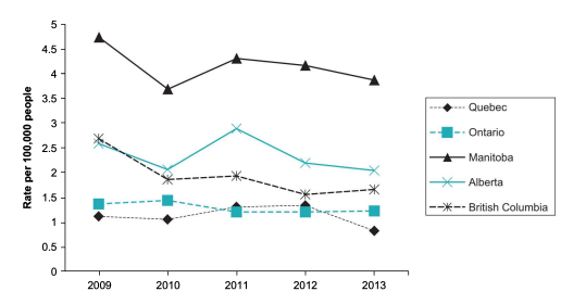
Since their invention over 200 years ago, line graphs have been recognized as being extremely useful for showing trends over time (Friendly \& Denis, 2005). When using it for this purpose, the creator of the line graph should use the horizontal axis to indicate time and the vertical axis to indicate the value of the variable being graphed. An example of this type of line graph is shown in Figure 3.24, which shows the murder rates in the five most populous Canadian provinces over the course of 5 years. Line graphs are also occasionally used to illustrate differences among categories or to display several variables at once. The latter purpose is common for line graphs because bar graphs and histograms can get too messy and complex when displaying more than one variable.
广义线性模型代写
统计代写|Generalized linear model代考广义线性模型代写|Frequency Polygons
直方图的另一种替代方法是箱线图(也称为盒须图),它是一种可视化模型,显示数据集中的分数是如何分散或紧凑的。图 3.21 显示了一个箱线图的示例,它代表了 Waite 等人的研究对象的年龄。(2015)研究。在箱线图中,有两个组成部分:箱(即图中心的矩形)和栅栏(从箱延伸的垂直线)。中间50%分数由方框表示。对于来自 Waite 等人的受试者年龄数据。(2015) 数据集,中间50%的分数范围从 21 到 31 ,所以如图所示的框3.21从 21 延伸到 31 。方框内是一条水平线,表示正好位于中间的分数,即 24 。较低的
围栏从盒子底部延伸到最低分数(即 18)。上栅栏从盒子的顶部延伸到最高分(38 分)。
图中的例子3.21显示了箱线图的一些有用特征,这些特征在直方图中并不总是很明显。首先,箱线图显示了分数的确切中间值。其次,箱线图显示了最小和最大分数与数据中间的距离。最后,很容易看出数据集中的分数是如何分布紧凑的。数字3.21表明 Waite 等人中最古老的科目。(2015)研究比最年轻的受试者离数据集的中间更远。这很明显,因为上围比下围长得多——表明最高分离中间远得多50%分数高于最低分数。
与频率多边形一样,箱线图的优点是可用于在同一张图片中显示多个变量。这是通过并排显示箱形图来完成的。在同一图中格式化多个箱形图可以很容易地确定哪些变量具有更高的均值和更广泛的分数范围。
统计代写|Generalized linear model代考广义线性模型代写|Stem-and-Leaf Plots
一些人用来显示数据的另一个可视化模型是茎叶图,图 3.23 右侧显示了一个示例。该图显示了表 3.1 中受试者的年龄。左列是十位(例如,数字 20 中的 2),其他列代表每个人年龄的个位(例如,数字 20 中的 0)。视觉模型右侧的每个数字代表一个人。要读取个人的分数,您可以将左栏中的数字与图表另一侧的数字结合起来。例如,这个样本中最年轻的人是 18 岁,如模型左栏中的 1 和右侧的 8 所示。第二个最年轻的人是 19 岁(由视觉模型左侧列中的 1 和右侧同一行中的 9 表示)。茎叶图还显示,有 7 人的年龄在 20 到 25 岁之间,其中最年长的人是 38 岁。在某种程度上,这个茎叶图类似于一个被翻转的直方图,每个间隔都是 10 年宽。
茎叶图可能很方便,但与直方图相比,它们有局限性。大型数据集可能会导致繁琐且难以阅读的茎叶图。如果变量的分数跨越广泛的值(例如,一些分数为个位数,其他分数为两位数或三位数)或精确测量的变量(其中大量受试者的分数为小数或分数),它们也可能存在问题.
在个人电脑普及之前,茎叶图更为常见,因为它们很容易在打字机上创建。随着能够自动生成直方图、频率多边形和箱线图的计算机软件的出现,茎叶图逐渐失去了人气。尽管如此,它们偶尔也会出现在现代社会科学研究文章中(例如,Acar, Sen, \& Cayirdag, 2016, p. 89; Linn, Graue, \& Sanders, 1990, p. 9; Paek, Abdulla, \& Cramond ,2016 年,第 125 页)。
统计代写|Generalized linear model代考广义线性模型代写|Line Graphs
另一种常见的定量数据可视化模型是折线图。与频率多边形一样,折线图是通过使用直线段将数据点相互连接来创建的。但是,折线图不必表示单个变量的连续值(如在频率多边形和直方图中),也不必以零频率开始和结束。折线图还可用于显示跨时间或跨名义或有序类别的趋势和差异。
自 200 多年前发明以来,线图已被认为对于显示随时间变化的趋势非常有用(Friendly \& Denis, 2005)。当用于此目的时,折线图的创建者应使用水平轴表示时间,使用垂直轴表示正在绘制的变量的值。图 3.24 显示了此类折线图的一个示例,该图显示了 5 年内加拿大人口最多的五个省份的谋杀率。折线图有时也用于说明类别之间的差异或一次显示多个变量。后一种用途对于折线图很常见,因为条形图和直方图在显示多个变量时会变得过于混乱和复杂。

统计代写请认准statistics-lab™. statistics-lab™为您的留学生涯保驾护航。
金融工程代写
金融工程是使用数学技术来解决金融问题。金融工程使用计算机科学、统计学、经济学和应用数学领域的工具和知识来解决当前的金融问题,以及设计新的和创新的金融产品。
非参数统计代写
非参数统计指的是一种统计方法,其中不假设数据来自于由少数参数决定的规定模型;这种模型的例子包括正态分布模型和线性回归模型。
广义线性模型代考
广义线性模型(GLM)归属统计学领域,是一种应用灵活的线性回归模型。该模型允许因变量的偏差分布有除了正态分布之外的其它分布。
术语 广义线性模型(GLM)通常是指给定连续和/或分类预测因素的连续响应变量的常规线性回归模型。它包括多元线性回归,以及方差分析和方差分析(仅含固定效应)。
有限元方法代写
有限元方法(FEM)是一种流行的方法,用于数值解决工程和数学建模中出现的微分方程。典型的问题领域包括结构分析、传热、流体流动、质量运输和电磁势等传统领域。
有限元是一种通用的数值方法,用于解决两个或三个空间变量的偏微分方程(即一些边界值问题)。为了解决一个问题,有限元将一个大系统细分为更小、更简单的部分,称为有限元。这是通过在空间维度上的特定空间离散化来实现的,它是通过构建对象的网格来实现的:用于求解的数值域,它有有限数量的点。边界值问题的有限元方法表述最终导致一个代数方程组。该方法在域上对未知函数进行逼近。[1] 然后将模拟这些有限元的简单方程组合成一个更大的方程系统,以模拟整个问题。然后,有限元通过变化微积分使相关的误差函数最小化来逼近一个解决方案。
tatistics-lab作为专业的留学生服务机构,多年来已为美国、英国、加拿大、澳洲等留学热门地的学生提供专业的学术服务,包括但不限于Essay代写,Assignment代写,Dissertation代写,Report代写,小组作业代写,Proposal代写,Paper代写,Presentation代写,计算机作业代写,论文修改和润色,网课代做,exam代考等等。写作范围涵盖高中,本科,研究生等海外留学全阶段,辐射金融,经济学,会计学,审计学,管理学等全球99%专业科目。写作团队既有专业英语母语作者,也有海外名校硕博留学生,每位写作老师都拥有过硬的语言能力,专业的学科背景和学术写作经验。我们承诺100%原创,100%专业,100%准时,100%满意。
随机分析代写
随机微积分是数学的一个分支,对随机过程进行操作。它允许为随机过程的积分定义一个关于随机过程的一致的积分理论。这个领域是由日本数学家伊藤清在第二次世界大战期间创建并开始的。
时间序列分析代写
随机过程,是依赖于参数的一组随机变量的全体,参数通常是时间。 随机变量是随机现象的数量表现,其时间序列是一组按照时间发生先后顺序进行排列的数据点序列。通常一组时间序列的时间间隔为一恒定值(如1秒,5分钟,12小时,7天,1年),因此时间序列可以作为离散时间数据进行分析处理。研究时间序列数据的意义在于现实中,往往需要研究某个事物其随时间发展变化的规律。这就需要通过研究该事物过去发展的历史记录,以得到其自身发展的规律。
回归分析代写
多元回归分析渐进(Multiple Regression Analysis Asymptotics)属于计量经济学领域,主要是一种数学上的统计分析方法,可以分析复杂情况下各影响因素的数学关系,在自然科学、社会和经济学等多个领域内应用广泛。
MATLAB代写
MATLAB 是一种用于技术计算的高性能语言。它将计算、可视化和编程集成在一个易于使用的环境中,其中问题和解决方案以熟悉的数学符号表示。典型用途包括:数学和计算算法开发建模、仿真和原型制作数据分析、探索和可视化科学和工程图形应用程序开发,包括图形用户界面构建MATLAB 是一个交互式系统,其基本数据元素是一个不需要维度的数组。这使您可以解决许多技术计算问题,尤其是那些具有矩阵和向量公式的问题,而只需用 C 或 Fortran 等标量非交互式语言编写程序所需的时间的一小部分。MATLAB 名称代表矩阵实验室。MATLAB 最初的编写目的是提供对由 LINPACK 和 EISPACK 项目开发的矩阵软件的轻松访问,这两个项目共同代表了矩阵计算软件的最新技术。MATLAB 经过多年的发展,得到了许多用户的投入。在大学环境中,它是数学、工程和科学入门和高级课程的标准教学工具。在工业领域,MATLAB 是高效研究、开发和分析的首选工具。MATLAB 具有一系列称为工具箱的特定于应用程序的解决方案。对于大多数 MATLAB 用户来说非常重要,工具箱允许您学习和应用专业技术。工具箱是 MATLAB 函数(M 文件)的综合集合,可扩展 MATLAB 环境以解决特定类别的问题。可用工具箱的领域包括信号处理、控制系统、神经网络、模糊逻辑、小波、仿真等。