如果你也在 怎样代写Generalized linear model这个学科遇到相关的难题,请随时右上角联系我们的24/7代写客服。
广义线性模型(GLiM,或GLM)是John Nelder和Robert Wedderburn在1972年提出的一种高级统计建模技术。它是一个包括许多其他模型的总称,它允许响应变量y具有正态分布以外的误差分布。
statistics-lab™ 为您的留学生涯保驾护航 在代写Generalized linear model方面已经树立了自己的口碑, 保证靠谱, 高质且原创的统计Statistics代写服务。我们的专家在代写Generalized linear model代写方面经验极为丰富,各种代写Generalized linear model相关的作业也就用不着说。
我们提供的Generalized linear model及其相关学科的代写,服务范围广, 其中包括但不限于:
- Statistical Inference 统计推断
- Statistical Computing 统计计算
- Advanced Probability Theory 高等概率论
- Advanced Mathematical Statistics 高等数理统计学
- (Generalized) Linear Models 广义线性模型
- Statistical Machine Learning 统计机器学习
- Longitudinal Data Analysis 纵向数据分析
- Foundations of Data Science 数据科学基础
统计代写|Generalized linear model代考广义线性模型代写|Models of Central Tendency
Models of central tendency are statistical models that are used to describe where the middle of the histogram lies. For many distributions, the model of central tendency is at or near the tallest bar in the histogram. (We will discuss exceptions to this general rule in the next chapter.) These statistical models are valuable in helping people understand their data because they show where most scores tend to cluster together. Models of central tendency are also important because they can help us understand the characteristics of the “typical” sample member.
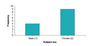
Mode. The most basic (and easiest to calculate) statistical model of central tendency is the mode. The mode of a variable is the most frequently occurring score in the data. For example, in the Waite et al. (2015) study that was used as an example in Chapter 3, there were four males (labeled as Group 1) and nine females (labeled as Group 2). Therefore, the mode for this variable is 2, or you could alternatively say that the mode sex of the sample is female. Modes are especially easy to find if the data are already in a frequency table because the mode will be the score that has the highest frequency value.
Calculating the mode requires at least nominal-level data. Remember from Chapter 2 that nominal data can be counted and classified (see Table 2.1). Because finding the mode merely requires counting the number of sample members who belong to each category, it makes sense that a mode can be calculated with nominal data. Additionally, any mathematical function that can be
performed with nominal data can be performed with all other levels of data, so a mode can also be calculated for ordinal, interval, and ratio data. This makes the mode the only model of central tendency that can be calculated for all levels of data, making the mode a useful and versatile statistical model.
One advantage of the mode is that it is not influenced by outliers. An outlier (also called an extreme value) is a member of a dataset that is unusual because its score is much higher or much lower than the other scores in the dataset (Cortina, 2002). Outliers can distort some statistical models, but not the mode because the mode is the most frequent score in the dataset. For an outlier to change the mode, there would have to be so many people with the same extreme score that it becomes the most common score in the dataset. If that were to happen, then these “outliers” would not be unusual.
The major disadvantage of the mode is that it cannot be used in later, more complex calculations in statistics. In other words, the mode is useful in its own right, but it cannot be used to create other statistical models that can provide additional information about the data.
统计代写|Generalized linear model代考广义线性模型代写|Models of Variability
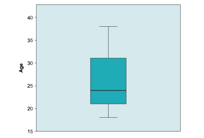
Statistical models of central tendency are useful, but they only communicate information about one characteristic of a variable: the location of the histogram’s center. Models of central tendency say nothing about another important characteristic of distributions – their variability. In statistics variability refers to the degree to which scores in a dataset vary from one another. Distributions with high variability tend to be spread out, while distributions with low variability tend to be compact. In this chapter we will discuss four models of variability: the range, the interquartile range, the standard deviation, and the variance.
Range. The range for a variable is the difference between the highest and the lowest scores in the dataset. Mathematically, this is:
$$
\text { Range }=\text { Highest Score – Lowest Score } \quad \text { (Formula 4.6) }
$$
The advantage of the range is that it is simple to calculate. But the disadvantages should also be apparent in the formula. First, only two scores (the highest score and the lowest score) determine the range. Although this does provide insight into the span of scores within a dataset, it does not say much (if anything) about the variability seen among the typical scores in the dataset. This is especially true if either the highest score or the lowest score is an outlier (or if both are outliers).
The second disadvantage of the range as a statistical model of variability is that outliers have more influence on the range than on any other statistical model discussed in this chapter. If either the highest score or the lowest score (or both) is an outlier, then the range can be greatly inflated and the data may appear to be more variable than they really are. Nevertheless, the range is still a useful statistical model of variability, especially in studies of growth or change, where it may show effectively whether sample members become more alike or grow in their differences over time.
A statistical assumption of the range is that the data are interval-or ratio-level data. This is because the formula for the range requires subtracting one score from another – a mathematical operation that requires interval data at a minimum.
Interquartile Range. Because the mean is extremely susceptible to the influence of outliers, a similar model of variability was developed in an attempt to overcome these shortfalls: the interquartile range, which is the range of the middle $50 \%$ of scores. There are three quartiles in any dataset, and these three scores divide the dataset into four equal-sized groups. These quartiles are (as numbered from the lowest score to the highest score) the first quartile, second quartile, and third quartile. ${ }^{1}$ There are four steps to finding the interquartile range:
- Calculate the median for a dataset. This is the second quartile.
- Find the score that is halfway between the median and the lowest score. This is the first quartile.
- Find the score that is halfway between the median and the highest score. This is the third quartile.
- Subtract the score in the first quartile from the third quartile to produce the interquartile range.
统计代写|Generalized linear model代考广义线性模型代写|Using Models of Central Tendency and Variance Together
Models of central tendency and models of variance provide different, but complementary information. Neither type of model can tell you everything you need to know about a distribution. However, when combined, these models can provide researchers with a thorough understanding of their data. For example, Figure $4.2$ shows two samples with the same mean, but one has a standard deviation that is twice as large as the other. Using just the mean to understand the two distributions would mask the important differences between the histograms. Indeed, when reporting a model of central tendency, it is recommended that you report an accompanying model of variability (Warne et al., 2012; Zientek,Capraro, \& Capraro, 2008). It is impossible to fully understand a distribution of scores without a knowledge of the variable’s central tendency and variability, and even slight differences in these values across distributions can be important (Voracek, Mohr, \& Hagmann, 2013).
This chapter discussed two types of descriptive statistics: models of central tendency and models of variability. Models of central tendency describe the location of the middle of the distribution, and models of variability describe the degree that scores are spread out from one another.
There were four models of central tendency in this chapter. Listed in ascending order of the complexity of their calculations, these are the mode, median, mean, and trimmed mean. The mode is calculated by finding the most frequent score in a dataset. The median is the center score when the data are arranged from the smallest score to the highest score (or vice versa). The mean is calculated by adding all the scores for a particular variable together and dividing by the number of scores. To find the trimmed mean, you should eliminate the same number of scores from the top and bottom of the distribution (usually $1 \%, 5 \%$, or $10 \%$ ) and then calculate the mean of the remaining data.
There were also four principal models of variability discussed in this chapter. The first was the range, which is found by subtracting the lowest score for a variable from the highest score for that same variable. The interquartile range requires finding the median and then finding the scores that are halfway between (a) the median and the lowest score in the dataset, and (b) the median and the highest score in the dataset. Score (a) is then subtracted from score (b). The standard deviation is defined as the square root of the average of the squared deviation scores of each individual in the dataset. Finally, the variance is defined as the square of the standard deviation (as a result, the variance is the mean of the squared deviation scores). There are three formulas for the standard deviation and three formulas for the variance in this chapter. Selecting the appropriate formula depends on (1) whether you have sample or population data, and (2) whether you wish to estimate the population standard deviation or variance.
No statistical model of central tendency or variability tells you everything you may need to know about your data. Only by using multiple models in conjunction with each other can you have a thorough understanding of your data.
广义线性模型代写
统计代写|Generalized linear model代考广义线性模型代写|Models of Central Tendency
集中趋势模型是用于描述直方图中间位置的统计模型。对于许多分布,集中趋势模型位于或接近直方图中最高的条形。(我们将在下一章讨论这个一般规则的例外情况。)这些统计模型对于帮助人们理解他们的数据很有价值,因为它们显示了大多数分数倾向于聚集在一起的位置。集中趋势模型也很重要,因为它们可以帮助我们理解“典型”样本成员的特征。
模式。集中趋势最基本(也是最容易计算)的统计模型是众数。变量的众数是数据中出现频率最高的分数。例如,在 Waite 等人中。(2015) 研究在第 3 章中用作示例,有 4 名男性(标记为第 1 组)和 9 名女性(标记为第 2 组)。因此,该变量的众数为 2,或者您也可以说样本的众数为女性。如果数据已经在频率表中,则模式特别容易找到,因为模式将是具有最高频率值的分数。
计算模式至少需要标称级别的数据。请记住第 2 章中的名义数据可以进行计数和分类(参见表 2.1)。因为找到众数只需要计算属于每个类别的样本成员的数量,所以可以用名义数据计算众数是有意义的。此外,任何数学函数都可以
用名义数据执行可以用所有其他级别的数据执行,因此也可以为序数、区间和比率数据计算众数。这使得该模式成为唯一可以计算所有级别数据的集中趋势模型,使该模式成为一个有用且通用的统计模型。
该模式的一个优点是它不受异常值的影响。异常值(也称为极值)是数据集的一个成员,它是不寻常的,因为它的分数比数据集中的其他分数高得多或低得多(Cortina,2002)。异常值会扭曲一些统计模型,但不会扭曲众数,因为众数是数据集中最常见的分数。对于改变模式的异常值,必须有很多人具有相同的极端分数,以至于它成为数据集中最常见的分数。如果发生这种情况,那么这些“异常值”就不会不寻常。
该模式的主要缺点是它不能用于以后更复杂的统计计算。换句话说,该模式本身很有用,但它不能用于创建可以提供有关数据的附加信息的其他统计模型。
统计代写|Generalized linear model代考广义线性模型代写|Models of Variability
集中趋势的统计模型很有用,但它们只传达有关变量的一个特征的信息:直方图中心的位置。集中趋势模型没有说明分布的另一个重要特征——它们的可变性。在统计中,可变性是指数据集中的分数彼此不同的程度。具有高变异性的分布往往是分散的,而具有低变异性的分布往往是紧凑的。在本章中,我们将讨论四种可变性模型:极差、四分位距、标准差和方差。
范围。变量的范围是数据集中最高分数和最低分数之间的差值。在数学上,这是:
范围 = 最高分 – 最低分 (公式 4.6)
范围的优点是计算简单。但缺点也应该在公式中很明显。首先,只有两个分数(最高分数和最低分数)确定范围。尽管这确实提供了对数据集中分数范围的洞察,但它并没有说明数据集中典型分数之间的可变性(如果有的话)。如果最高分数或最低分数是异常值(或两者都是异常值),则尤其如此。
范围作为可变性统计模型的第二个缺点是,与本章讨论的任何其他统计模型相比,离群值对范围的影响更大。如果最高分或最低分(或两者)是异常值,则范围可能会大大膨胀,并且数据可能看起来比实际情况更具可变性。尽管如此,该范围仍然是一个有用的变异性统计模型,特别是在增长或变化的研究中,它可以有效地显示样本成员是否随着时间的推移变得更加相似或差异增加。
范围的统计假设是数据是区间或比率级别的数据。这是因为范围的公式需要从另一个分数中减去一个分数——这是一种至少需要区间数据的数学运算。
四分位距。由于均值极易受到异常值的影响,因此开发了一个类似的可变性模型以试图克服这些不足:四分位距,即中间值的范围50%的分数。任何数据集中都有三个四分位数,这三个分数将数据集分成四个大小相等的组。这些四分位数是(从最低分到最高分编号)第一个四分位数、第二个四分位数和第三个四分位数。1找到四分位距有四个步骤:
- 计算数据集的中位数。这是第二个四分位数。
- 找到中位数和最低分数之间的分数。这是第一个四分位数。
- 找到中位数和最高分之间的分数。这是第三个四分位数。
- 从第三个四分位数中减去第一个四分位数的分数以产生四分位数范围。
统计代写|Generalized linear model代考广义线性模型代写|Using Models of Central Tendency and Variance Together
集中趋势模型和方差模型提供了不同但互补的信息。两种类型的模型都无法告诉您您需要了解的有关分布的所有信息。然而,当结合起来时,这些模型可以让研究人员彻底了解他们的数据。例如,图4.2显示具有相同平均值的两个样本,但一个样本的标准差是另一个样本的两倍。仅使用均值来理解这两个分布会掩盖直方图之间的重要差异。实际上,在报告集中趋势模型时,建议您报告伴随的可变性模型(Warne 等人,2012;Zientek,Capraro,\& Capraro,2008)。如果不了解变量的集中趋势和可变性,就不可能完全理解分数的分布,即使这些值在分布之间的微小差异也很重要(Voracek, Mohr, \& Hagmann, 2013)。
本章讨论了两种类型的描述性统计:集中趋势模型和变异模型。集中趋势模型描述了分布中间的位置,而变异模型描述了分数彼此分散的程度。
本章有四种集中趋势模型。按计算复杂度的升序排列,它们是众数、中位数、均值和修剪后的均值。该模式是通过在数据集中找到最频繁的分数来计算的。中位数是当数据从最小分数到最高分数(反之亦然)排列时的中心分数。平均值是通过将特定变量的所有分数相加并除以分数数来计算的。要找到修剪后的平均值,您应该从分布的顶部和底部消除相同数量的分数(通常1%,5%, 或者10%) 然后计算剩余数据的平均值。
本章还讨论了四种主要的可变性模型。第一个是范围,它是通过从同一变量的最高分数中减去一个变量的最低分数来找到的。四分位数范围需要找到中位数,然后找到介于 (a) 数据集中的中位数和最低分数之间的分数,以及 (b) 数据集中的中位数和最高分数之间的分数。然后从分数 (b) 中减去分数 (a)。标准偏差定义为数据集中每个个体的平方偏差分数的平均值的平方根。最后,方差定义为标准差的平方(因此,方差是平方差得分的平均值)。本章中有标准差的三个公式和方差的三个公式。
没有集中趋势或可变性的统计模型可以告诉您您可能需要了解的有关数据的所有信息。只有将多个模型相互结合使用,才能对数据有一个透彻的了解。

统计代写请认准statistics-lab™. statistics-lab™为您的留学生涯保驾护航。
金融工程代写
金融工程是使用数学技术来解决金融问题。金融工程使用计算机科学、统计学、经济学和应用数学领域的工具和知识来解决当前的金融问题,以及设计新的和创新的金融产品。
非参数统计代写
非参数统计指的是一种统计方法,其中不假设数据来自于由少数参数决定的规定模型;这种模型的例子包括正态分布模型和线性回归模型。
广义线性模型代考
广义线性模型(GLM)归属统计学领域,是一种应用灵活的线性回归模型。该模型允许因变量的偏差分布有除了正态分布之外的其它分布。
术语 广义线性模型(GLM)通常是指给定连续和/或分类预测因素的连续响应变量的常规线性回归模型。它包括多元线性回归,以及方差分析和方差分析(仅含固定效应)。
有限元方法代写
有限元方法(FEM)是一种流行的方法,用于数值解决工程和数学建模中出现的微分方程。典型的问题领域包括结构分析、传热、流体流动、质量运输和电磁势等传统领域。
有限元是一种通用的数值方法,用于解决两个或三个空间变量的偏微分方程(即一些边界值问题)。为了解决一个问题,有限元将一个大系统细分为更小、更简单的部分,称为有限元。这是通过在空间维度上的特定空间离散化来实现的,它是通过构建对象的网格来实现的:用于求解的数值域,它有有限数量的点。边界值问题的有限元方法表述最终导致一个代数方程组。该方法在域上对未知函数进行逼近。[1] 然后将模拟这些有限元的简单方程组合成一个更大的方程系统,以模拟整个问题。然后,有限元通过变化微积分使相关的误差函数最小化来逼近一个解决方案。
tatistics-lab作为专业的留学生服务机构,多年来已为美国、英国、加拿大、澳洲等留学热门地的学生提供专业的学术服务,包括但不限于Essay代写,Assignment代写,Dissertation代写,Report代写,小组作业代写,Proposal代写,Paper代写,Presentation代写,计算机作业代写,论文修改和润色,网课代做,exam代考等等。写作范围涵盖高中,本科,研究生等海外留学全阶段,辐射金融,经济学,会计学,审计学,管理学等全球99%专业科目。写作团队既有专业英语母语作者,也有海外名校硕博留学生,每位写作老师都拥有过硬的语言能力,专业的学科背景和学术写作经验。我们承诺100%原创,100%专业,100%准时,100%满意。
随机分析代写
随机微积分是数学的一个分支,对随机过程进行操作。它允许为随机过程的积分定义一个关于随机过程的一致的积分理论。这个领域是由日本数学家伊藤清在第二次世界大战期间创建并开始的。
时间序列分析代写
随机过程,是依赖于参数的一组随机变量的全体,参数通常是时间。 随机变量是随机现象的数量表现,其时间序列是一组按照时间发生先后顺序进行排列的数据点序列。通常一组时间序列的时间间隔为一恒定值(如1秒,5分钟,12小时,7天,1年),因此时间序列可以作为离散时间数据进行分析处理。研究时间序列数据的意义在于现实中,往往需要研究某个事物其随时间发展变化的规律。这就需要通过研究该事物过去发展的历史记录,以得到其自身发展的规律。
回归分析代写
多元回归分析渐进(Multiple Regression Analysis Asymptotics)属于计量经济学领域,主要是一种数学上的统计分析方法,可以分析复杂情况下各影响因素的数学关系,在自然科学、社会和经济学等多个领域内应用广泛。
MATLAB代写
MATLAB 是一种用于技术计算的高性能语言。它将计算、可视化和编程集成在一个易于使用的环境中,其中问题和解决方案以熟悉的数学符号表示。典型用途包括:数学和计算算法开发建模、仿真和原型制作数据分析、探索和可视化科学和工程图形应用程序开发,包括图形用户界面构建MATLAB 是一个交互式系统,其基本数据元素是一个不需要维度的数组。这使您可以解决许多技术计算问题,尤其是那些具有矩阵和向量公式的问题,而只需用 C 或 Fortran 等标量非交互式语言编写程序所需的时间的一小部分。MATLAB 名称代表矩阵实验室。MATLAB 最初的编写目的是提供对由 LINPACK 和 EISPACK 项目开发的矩阵软件的轻松访问,这两个项目共同代表了矩阵计算软件的最新技术。MATLAB 经过多年的发展,得到了许多用户的投入。在大学环境中,它是数学、工程和科学入门和高级课程的标准教学工具。在工业领域,MATLAB 是高效研究、开发和分析的首选工具。MATLAB 具有一系列称为工具箱的特定于应用程序的解决方案。对于大多数 MATLAB 用户来说非常重要,工具箱允许您学习和应用专业技术。工具箱是 MATLAB 函数(M 文件)的综合集合,可扩展 MATLAB 环境以解决特定类别的问题。可用工具箱的领域包括信号处理、控制系统、神经网络、模糊逻辑、小波、仿真等。