如果你也在 怎样代写三维成像Three-Dimensional Imaging这个学科遇到相关的难题,请随时右上角联系我们的24/7代写客服。
三维成像是一种将许多扫描(来自计算机断层扫描、核磁共振或超声扫描)通过计算结合起来的技术。然后,这些图像可以由放射科医师或医生进行操作,以帮助诊断和手术计划。
statistics-lab™ 为您的留学生涯保驾护航 在代写三维成像Three-Dimensional Imaging方面已经树立了自己的口碑, 保证靠谱, 高质且原创的统计Statistics代写服务。我们的专家在代写三维成像Three-Dimensional Imaging方面经验极为丰富,各种代写三维成像Three-Dimensional Imaging相关的作业也就用不着说。
我们提供的三维成像Three-Dimensional Imaging及其相关学科的代写,服务范围广, 其中包括但不限于:
- Statistical Inference 统计推断
- Statistical Computing 统计计算
- Advanced Probability Theory 高等楖率论
- Advanced Mathematical Statistics 高等数理统计学
- (Generalized) Linear Models 广义线性模型
- Statistical Machine Learning 统计机器学习
- Longitudinal Data Analysis 纵向数据分析
- Foundations of Data Science 数据科学基础
电子工程代写|三维成像代写Three-Dimensional Imaging代考|Geometric Approach
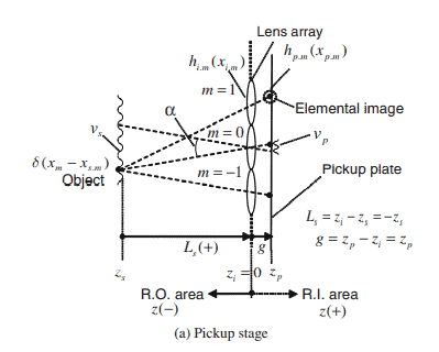
Though the principle of image formation is described above, a more thorough explanation must include a description of ray tracing by geometrical optics $[11,12]$. Figures 1.1(a) and (b) focus on around the $m$-th elemental lenses, many of which constitute an array. A point light source is placed at distance $L_{s}$ from the lens array and is expressed as a delta function $\delta\left(x_{m}-x_{s, m}\right)$, where $x_{s . m}$ represents the object’s position. $x_{i . m}$ and $x_{p . m}$ represent the positions in the incident plane of the lens array and capture plate, respectively. Subscript $m$ indicates the position on the coordinates where the intersection of an incident plane and its own optical axis is the origin for each elemental lens. The following $x$ can be obtained by adding $m P_{a}$ to $x_{m}$, that is, the distance from the origin of the whole array to the optical axis of the elemental lens:
$$
x=x_{m}+m P_{a},
$$
where $x_{s, m}, x_{i, m}$ and $x_{p, m}$ are converted to $x_{s}, x_{i}$ and $x_{p}$, respectively, by adding $m P_{a}$ in the same way. $P_{a}$ is the pitch between adjacent elemental lenses. Note that $z$ is not assigned a subscript because the coordinates of each elemental lens match those of the whole array. The origin of the $x$ and $z$ coordinates of the whole array is defined as the point where the optical axis crosses the incident plane of the central elemental lens. To simplify calculations, we use the two-dimensional coordinates $(x, z)$, defined by the $x$-axis and optical axis $z$.
Real objects in the capture stage can be located in the space with a negative value of $z$, which is called the real objects area (R.O. area). Real images in the display stage can be located in the space with a positive value of $z$, which is called the real images area (R.I. area). The following calculations can be applied to the three-dimensional coordinates $(x, y, z)$ defined by the optical axis and a plane that crosses it perpendicularly. There is a relationship between $x_{s . m}$ and $x_{p . m}$ in the capture stage shown in Fig. 1.1(a):
$$
\frac{x_{s . m}}{z_{s}}=\frac{x_{p . m}}{g},
$$
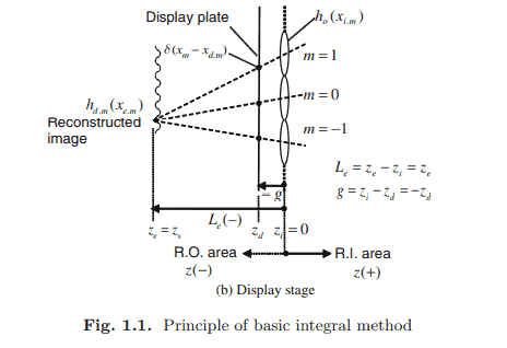
where $g$ is the gap between the elemental lens and the capture plate. As shown in Fig. 1.1(b), we assume the pitch of the elemental lenses and the gap in the display stage are the same as in the capture stage, respectively. $x_{d, m}$ is the position of the point light source in the display plate and $x_{m}$ represents the space in which the reconstructed image is formed. There is a similar relationship between $x_{d, m}$ and $x_{m}$ in the display stage:
$$
-\frac{x_{d . m}}{g}=\frac{x_{m}}{z}
$$
电子工程代写|三维成像代写Three-Dimensional Imaging代考|Wave Optical Approach
By using wave optics the captured elemental images synthesize an optical image in the display stage $[16,17]$. We present the response of the $m$-th elemental lens on the pickup plate shown in Fig. 1.1(a). First, the wave (electric field) entering the elemental lens of the pickup stage is calculated by Fresnel’s approximation as
$$
\begin{aligned}
u_{i, m}\left(x_{i . m}\right)=& \frac{1}{j \lambda L_{s}} \exp \left(-j k \frac{x_{i, m}^{2}}{2 L_{s}}\right) \int_{o b j e c t} \delta\left(x_{m}-x_{s . m}\right) \exp \left(-j k \frac{x_{m}^{2}}{2 L_{s}}\right) \
& \exp \left(-j k \frac{x_{m} x_{i, m}}{L_{s}}\right) d x_{m} \
=& \frac{1}{j \lambda L_{s}} \exp \left(-j k \frac{x_{i, m}^{2}}{2 L_{s}}\right) \exp \left(-j k \frac{x_{s, m}^{2}}{2 L_{s}}\right) e\left(-j k \frac{x_{s, m} x_{i . m}}{L_{s}}\right)
\end{aligned}
$$
where $L_{s}=Z_{i}-Z_{s}, k$ is the wave number and equals $2 \pi / \lambda$, and $\lambda$ is the wavelength. The output wave from an elemental lens is a product of Eq. (1.8) and the phase shift function of the elemental lens:
$$
u_{i, m}\left(x_{i, m}\right) \exp \left(x_{i, m}^{2} / 2 f\right) .
$$
The wave on the capture plate is obtained by
$$
\begin{aligned}
&h_{p . m}\left(x_{p . m}\right)=\frac{1}{j \lambda g} \exp \left(-j k \frac{x_{p . m}^{2}}{2 g}\right) \int_{-w_{a / 2}}^{w_{a / 2}} u_{i . m}\left(x_{i . m}\right) \exp \left(\frac{x_{i, m}^{2}}{2 f}\right) \exp \left(-j k \frac{x_{i, m}^{2}}{2 g}\right) \
&\quad \exp \left(-j k \frac{x_{i, m} x_{p . m}}{g}\right) d x_{i . m},
\end{aligned}
$$
where $f$ is the focal length of the elemental lens, and $w_{a}$ is the width of an elemental lens.
三维成像代考
电子工程代写|三维成像代写Three-Dimensional Imaging代考|Geometric Approach
虽然上面描述了成像的原理,但更彻底的解释必须包括几何光学对光线追踪的描述 $[11,12]$. 图 1.1(a) 和 (b) 集中在 $m$-th元素透镜,其中许多构成一个阵列。点光源放置在远处 $L_{s}$ 来自透镜阵列,并表示为 delta 函数
$\delta\left(x_{m}-x_{s, m}\right)$ ,在哪里 $x_{s . m}$ 表示对象的位置。 $x_{i . m}$ 和 $x_{p . m}$ 分别表示透镱阵列和捕获板在入射平面中的位置。下 标 $m$ 表示在坐标上的位置,其中入射平面和它自己的光轴的交点是每个元素透镜的原点。以下 $x$ 可以通过添加获得 $m P_{a}$ 至 $x_{m}$ ,即整个阵列的原点到基本透镜光轴的距离:
$$
x=x_{m}+m P_{a},
$$
在哪里 $x_{s, m}, x_{i, m}$ 和 $x_{p, m}$ 被转换为 $x_{s}, x_{i}$ 和 $x_{p}$ ,分别通过添加 $m P_{a}$ 以同样的方式。 $P_{a}$ 是相邻元素透镜之间的间 距。注意 $z$ 没有指定下标,因为每个基本透镜的坐标与整个阵列的坐标相匹配。的由来 $x$ 和 $z$ 整个阵列的坐标定义为 光轴与中心元素透镜的入射平面相交的点。为了简化计算,我们使用二维坐标 $(x, z)$ ,由 $x$ 轴和光轴 $z$.
捕获阶段的真实对象可以位于具有负值的空间中 $z$ ,称为真实对象区域 (RO 区域)。展示阶段的真实图像可以位 于具有正值的空间中 $z$ ,称为真实图像区域 (RI 区域)。以下计算可应用于三维坐标 $(x, y, z)$ 由光轴和与其垂直相 交的平面定义。之间有关系 $x_{s . m}$ 和 $x_{p . m}$ 在图 1.1(a) 所示的捕获阶段:
$$
\frac{x_{s . m}}{z_{s}}=\frac{x_{p . m}}{g},
$$
在哪里 $g$ 是基本透镜和捕获板之间的间隙。如图 $1.1$ (b) 所示,我们假设显示阶段的基本透镜间距和间隙分别与捕获 阶段相同。 $x_{d, m}$ 是点光源在显示板中的位置, $x_{m}$ 表示形成重建图像的空间。之间也有类似的关系 $x_{d, m}$ 和 $x_{m}$ 在展 示阶段:
$$
-\frac{x_{d . m}}{g}=\frac{x_{m}}{z}
$$
电子工程代写|三维成像代写Three-Dimensional Imaging代考|Wave Optical Approach
通过使用波动光学,捕获的元素图像在显示阶段合成光学图像 $[16,17]$. 我们提出了 $m$ 图 1.1(a) 所示的拾取板上的 第一个基本透镜。首先,通过菲涅耳近似计算进入拾取台的基本透镜的波 (电场) 为
$$
u_{i, m}\left(x_{i . m}\right)=\frac{1}{j \lambda L_{s}} \exp \left(-j k \frac{x_{i, m}^{2}}{2 L_{s}}\right) \int_{\text {object }} \delta\left(x_{m}-x_{s . m}\right) \exp \left(-j k \frac{x_{m}^{2}}{2 L_{s}}\right) \quad \exp \left(-j k \frac{x_{m} x_{i, m}}{L_{s}}\right) d x_{r}
$$
在哪里 $L_{s}=Z_{i}-Z_{s}, k$ 是波数,等于 $2 \pi / \lambda$ ,和 $\lambda$ 是波长。元素透镜的输出波是等式的乘积。(1.8)和元素透镜的 相移函数:
$$
u_{i, m}\left(x_{i, m}\right) \exp \left(x_{i, m}^{2} / 2 f\right) .
$$
捕获板上的波由下式获得
$$
h_{p . m}\left(x_{p . m}\right)=\frac{1}{j \lambda g} \exp \left(-j k \frac{x_{p, m}^{2}}{2 g}\right) \int_{-w_{a / 2}}^{w_{a / 2}} u_{i . m}\left(x_{i . m}\right) \exp \left(\frac{x_{i, m}^{2}}{2 f}\right) \exp \left(-j k \frac{x_{i, m}^{2}}{2 g}\right) \quad \exp (-j k .
$$
在哪里 $f$ 是元素透镜的焦距,并且 $w_{a}$ 是元素透镜的宽度。

统计代写请认准statistics-lab™. statistics-lab™为您的留学生涯保驾护航。统计代写|python代写代考
随机过程代考
在概率论概念中,随机过程是随机变量的集合。 若一随机系统的样本点是随机函数,则称此函数为样本函数,这一随机系统全部样本函数的集合是一个随机过程。 实际应用中,样本函数的一般定义在时间域或者空间域。 随机过程的实例如股票和汇率的波动、语音信号、视频信号、体温的变化,随机运动如布朗运动、随机徘徊等等。
贝叶斯方法代考
贝叶斯统计概念及数据分析表示使用概率陈述回答有关未知参数的研究问题以及统计范式。后验分布包括关于参数的先验分布,和基于观测数据提供关于参数的信息似然模型。根据选择的先验分布和似然模型,后验分布可以解析或近似,例如,马尔科夫链蒙特卡罗 (MCMC) 方法之一。贝叶斯统计概念及数据分析使用后验分布来形成模型参数的各种摘要,包括点估计,如后验平均值、中位数、百分位数和称为可信区间的区间估计。此外,所有关于模型参数的统计检验都可以表示为基于估计后验分布的概率报表。
广义线性模型代考
广义线性模型(GLM)归属统计学领域,是一种应用灵活的线性回归模型。该模型允许因变量的偏差分布有除了正态分布之外的其它分布。
statistics-lab作为专业的留学生服务机构,多年来已为美国、英国、加拿大、澳洲等留学热门地的学生提供专业的学术服务,包括但不限于Essay代写,Assignment代写,Dissertation代写,Report代写,小组作业代写,Proposal代写,Paper代写,Presentation代写,计算机作业代写,论文修改和润色,网课代做,exam代考等等。写作范围涵盖高中,本科,研究生等海外留学全阶段,辐射金融,经济学,会计学,审计学,管理学等全球99%专业科目。写作团队既有专业英语母语作者,也有海外名校硕博留学生,每位写作老师都拥有过硬的语言能力,专业的学科背景和学术写作经验。我们承诺100%原创,100%专业,100%准时,100%满意。
机器学习代写
随着AI的大潮到来,Machine Learning逐渐成为一个新的学习热点。同时与传统CS相比,Machine Learning在其他领域也有着广泛的应用,因此这门学科成为不仅折磨CS专业同学的“小恶魔”,也是折磨生物、化学、统计等其他学科留学生的“大魔王”。学习Machine learning的一大绊脚石在于使用语言众多,跨学科范围广,所以学习起来尤其困难。但是不管你在学习Machine Learning时遇到任何难题,StudyGate专业导师团队都能为你轻松解决。
多元统计分析代考
基础数据: $N$ 个样本, $P$ 个变量数的单样本,组成的横列的数据表
变量定性: 分类和顺序;变量定量:数值
数学公式的角度分为: 因变量与自变量
时间序列分析代写
随机过程,是依赖于参数的一组随机变量的全体,参数通常是时间。 随机变量是随机现象的数量表现,其时间序列是一组按照时间发生先后顺序进行排列的数据点序列。通常一组时间序列的时间间隔为一恒定值(如1秒,5分钟,12小时,7天,1年),因此时间序列可以作为离散时间数据进行分析处理。研究时间序列数据的意义在于现实中,往往需要研究某个事物其随时间发展变化的规律。这就需要通过研究该事物过去发展的历史记录,以得到其自身发展的规律。
回归分析代写
多元回归分析渐进(Multiple Regression Analysis Asymptotics)属于计量经济学领域,主要是一种数学上的统计分析方法,可以分析复杂情况下各影响因素的数学关系,在自然科学、社会和经济学等多个领域内应用广泛。
MATLAB代写
MATLAB 是一种用于技术计算的高性能语言。它将计算、可视化和编程集成在一个易于使用的环境中,其中问题和解决方案以熟悉的数学符号表示。典型用途包括:数学和计算算法开发建模、仿真和原型制作数据分析、探索和可视化科学和工程图形应用程序开发,包括图形用户界面构建MATLAB 是一个交互式系统,其基本数据元素是一个不需要维度的数组。这使您可以解决许多技术计算问题,尤其是那些具有矩阵和向量公式的问题,而只需用 C 或 Fortran 等标量非交互式语言编写程序所需的时间的一小部分。MATLAB 名称代表矩阵实验室。MATLAB 最初的编写目的是提供对由 LINPACK 和 EISPACK 项目开发的矩阵软件的轻松访问,这两个项目共同代表了矩阵计算软件的最新技术。MATLAB 经过多年的发展,得到了许多用户的投入。在大学环境中,它是数学、工程和科学入门和高级课程的标准教学工具。在工业领域,MATLAB 是高效研究、开发和分析的首选工具。MATLAB 具有一系列称为工具箱的特定于应用程序的解决方案。对于大多数 MATLAB 用户来说非常重要,工具箱允许您学习和应用专业技术。工具箱是 MATLAB 函数(M 文件)的综合集合,可扩展 MATLAB 环境以解决特定类别的问题。可用工具箱的领域包括信号处理、控制系统、神经网络、模糊逻辑、小波、仿真等。