如果你也在 怎样代写机器学习 machine learning这个学科遇到相关的难题,请随时右上角联系我们的24/7代写客服。
机器学习是一个致力于理解和建立 “学习 “方法的研究领域,也就是说,利用数据来提高某些任务的性能的方法。机器学习算法基于样本数据(称为训练数据)建立模型,以便在没有明确编程的情况下做出预测或决定。机器学习算法被广泛用于各种应用,如医学、电子邮件过滤、语音识别和计算机视觉,在这些应用中,开发传统算法来执行所需任务是困难的或不可行的。
statistics-lab™ 为您的留学生涯保驾护航 在代写机器学习 machine learning方面已经树立了自己的口碑, 保证靠谱, 高质且原创的统计Statistics代写服务。我们的专家在代写机器学习 machine learning代写方面经验极为丰富,各种代写机器学习 machine learning相关的作业也就用不着说。
我们提供的机器学习 machine learning及其相关学科的代写,服务范围广, 其中包括但不限于:
- Statistical Inference 统计推断
- Statistical Computing 统计计算
- Advanced Probability Theory 高等概率论
- Advanced Mathematical Statistics 高等数理统计学
- (Generalized) Linear Models 广义线性模型
- Statistical Machine Learning 统计机器学习
- Longitudinal Data Analysis 纵向数据分析
- Foundations of Data Science 数据科学基础
机器学习代考_Machine Learning代考_Deep metric learning
When measuring the distance between high-dimensional or structured inputs, it is very useful to first learn an embedding to a lower dimensional “semantic” space, where distances are more meaningful, and less subject to the curse of dimensionality (Section 16.1.2). Let $\boldsymbol{e}=f(\boldsymbol{x} ; \boldsymbol{\theta}) \in \mathbb{R}^L$ be an embedding of the input that preserves the “relevant” semantic aspects of the input, and let $\hat{e}=\boldsymbol{e} /|\boldsymbol{e}|_2$ be the $\ell_2$-normalized version. This ensures that all points lie on a hyper-sphere. We can then measure the distance between two points using the normalized Euclidean distance
$$
d\left(\boldsymbol{x}_i, \boldsymbol{x}_j ; \boldsymbol{\theta}\right)=\left|\hat{\boldsymbol{e}}_i-\hat{\boldsymbol{e}}_j\right|_2^2
$$
where smaller values means more similar, or the cosine similarity
$$
d\left(\boldsymbol{x}_i, \boldsymbol{x}_j ; \boldsymbol{\theta}\right)=\hat{e}_i^{\mathrm{T}} \hat{e}_j
$$
where larger values means more similar. (Cosine similarity measures the angle between the two vectors, as illustrated in Figure 20.43.) These quantities are related via
$$
\left|\hat{e}_i-\hat{e}_j\right|_2^2=\left(\hat{e}_i-\hat{e}_j\right)^{\mathrm{T}}\left(\hat{e}_i-\hat{e}_j\right)=2-2 \hat{e}_i^{\mathrm{T}} \hat{\boldsymbol{e}}_j
$$
This overall approach is called deep metric learning or DML.
The basic idea in DML is to learn the embedding function such that similar examples are closer than dissimilar examples. More precisely, we assume we have a labeled dataset, $\mathcal{D}=\left{\left(\boldsymbol{x}_i, y_i\right): i=1: N\right}$, from which we can derive a set of similar pairs, $\mathcal{S}=\left{(i, j): y_i=y_j\right}$. If $(i, j) \in \mathcal{S}$ but $(i, k) \notin S$, then we assume that $\boldsymbol{x}_i$ and $\boldsymbol{x}_j$ should be close in embedding space, whereas $\boldsymbol{x}_i$ and $\boldsymbol{x}_k$ should be far. We discuss various ways to enforce this property below. Note that these methods also work when we do not have class labels, provided we have some other way of defining similar pairs. For example, in Section 19.2.4.3, we discuss self-supervised approaches to representation learning, that automatically create semantically similar pairs, and learn embeddings to force these pairs to be closer than unrelated pairs.
Before discussing DML in more detail, it is worth mentioning that many recent approaches to DML are not as good as they claim to be, as pointed out in [MBL20; Rot+20]. (The claims in some of these papers are often invalid due to improper experimental comparisons, a common flaw in contemporary ML research, as discussed in e.g., [BLV19; LS19b].) We therefore focus on (slightly) older and simpler methods, that tend to be more robust.
机器学习代考_Machine Learning代考_Optimizing an upper bound
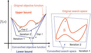
$[$ Do $+19]$ proposed a simple and fast method for optimizing the triplet loss. The key idea is to define one fixed proxy or centroid per class, and then to use distance to the proxy as an upper bound on the triplet loss.
More precisely, consider a simplified form of the triplet loss, without the margin term:
$$
\ell_t\left(\boldsymbol{x}i, \boldsymbol{x}_j, \boldsymbol{x}_k\right)=\left|\hat{\boldsymbol{e}}_i-\hat{\boldsymbol{e}}_j\right|-\left|\hat{\boldsymbol{e}}_i-\hat{\boldsymbol{e}}_k\right| $$ where $\hat{\boldsymbol{e}}_i=\hat{e}\theta\left(\boldsymbol{x}i\right)$, etc. Using the triangle inequality we have $$ \begin{aligned} &\left|\hat{e}_i-\hat{e}_j\right| \leq\left|\hat{e}_i-c{y_i}\right|+\left|\hat{\boldsymbol{e}}j-c{y_i}\right| \
&\left|\hat{e}i-\hat{\boldsymbol{e}}_k\right| \geq\left|\hat{\boldsymbol{e}}_i-c{y_k}\right|-\left|\hat{\boldsymbol{e}}k-c{y_k}\right|
\end{aligned}
$$
Hence
$$
\ell_t\left(\boldsymbol{x}i, \boldsymbol{x}_j, \boldsymbol{x}_k\right) \leq \ell_u\left(\boldsymbol{x}_i, \boldsymbol{x}_j, \boldsymbol{x}_k\right) \triangleq\left|\hat{\boldsymbol{e}}_i-\boldsymbol{c}{y_i}\right|-\left|\hat{\boldsymbol{e}}i-\boldsymbol{c}{y_k}\right|+\left|\hat{\boldsymbol{e}}j-\boldsymbol{c}{y_i}\right|+\left|\hat{\boldsymbol{e}}k-\boldsymbol{c}{y_k}\right|
$$
We can use this to derive a tractable upper bound on the triplet loss as follows:
$$
\begin{aligned}
\mathcal{L}t(\mathcal{D}, \mathcal{S}) &=\sum{(i, j) \in \mathcal{S},(i, k) \notin \mathcal{S}, i, j, k \in{1, \ldots, N}} \ell_t\left(\boldsymbol{x}i, \boldsymbol{x}_j, \boldsymbol{x}_k\right) \leq \sum{(i, j) \in \mathcal{S},(i, k) \notin \mathcal{S}, i, j, k \in{1, \ldots, N}} \ell_u\left(\boldsymbol{x}i, \boldsymbol{x}_j, \boldsymbol{x}_k\right) \ &=C^{\prime} \sum{i=1}^N\left(\left|\boldsymbol{x}i-\boldsymbol{c}{y_i}\right|-\frac{1}{3(C-1)} \sum_{m=1, m \neq y_i}^C\left|\boldsymbol{x}_i-\boldsymbol{c}_m\right|\right) \triangleq \mathcal{L}_u(\mathcal{D}, \mathcal{S})
\end{aligned}
$$
where $C^{\prime}=3(C-1)\left(\frac{N}{C}-1\right) \frac{N}{C}$ is a constant. It is clear that $\mathcal{L}_u$ can be computed in $O(N C)$ time. See Figure 16.6b for an illustration.
In [Do+19], they show that $0 \leq \mathcal{L}_t-\mathcal{L}_u \leq \frac{N^3}{C^2} K$, where $K$ is some constant that depends on the spread of the centroids. To ensure the bound is tight, the centroids should be as far from each other as possible, and the distances between them should be as similar as possible. An easy way to ensure is to define the $c_m$ vectors to be one-hot vectors, one per class. These vectors already have unit norm, and are orthogonal to each other. The distance between each pair of centroids is $\sqrt{2}$, which ensures the upper bound is fairly tight.
The downside of this approach is that it assumes the embedding layer is $L=C$ dimensional. There are two solutions to this. First, after training, we can add a linear projection layer to map from $C$ to $L \neq C$, or we can take the second-to-last layer of the embedding network. The second approach is to sample a large number of points on the $L$-dimensional unit hyper-sphere (which we can do by sampling from the standard normal, and then normalizing [Mar72]), and then running K-means clustering (Section 21.3) with $K=C$. In the experiments reported in [Do+19], these two approaches give similar results.
机器学习代考
机器学习代考_Machine Learning代考_Deep metric learning
在测量高维或结构化输入之间的距离时,首先学习到低维”语义”空间的嵌入非常有用,在该空间中距离更有意 义,并且较少受到维数灾难的影响 (第 16.1.2 节) . 让e $=f(\boldsymbol{x} ; \boldsymbol{\theta}) \in \mathbb{R}^L$ 是保留输入的“相关”语义方面的输入 的嵌入,并且让 $\hat{e}=\boldsymbol{e} /|\boldsymbol{e}|_2$ 成为 $\ell_2$-规范化版本。这确保所有点都位于超球面上。然后我们可以使用归一化欧氏 距离测量两点之间的距离
$$
d\left(\boldsymbol{x}_i, \boldsymbol{x}_j ; \boldsymbol{\theta}\right)=\left|\hat{\boldsymbol{e}}_i-\hat{\boldsymbol{e}}_j\right|_2^2
$$
其中较小的值意味着更相似,或余弦相似度
$$
d\left(\boldsymbol{x}_i, \boldsymbol{x}_j ; \boldsymbol{\theta}\right)=\hat{e}_i^{\mathrm{T}} \hat{e}_j
$$
其中较大的值意味着更相似。(余弦相似度测量两个向量之间的角度,如图 $20.43$ 所示。)这些量通过
$$
\left|\hat{e}_i-\hat{e}_j\right|_2^2=\left(\hat{e}_i-\hat{e}_j\right)^{\mathrm{T}}\left(\hat{e}_i-\hat{e}_j\right)=2-2 \hat{e}_i^{\mathrm{T}} \hat{\boldsymbol{e}}_j
$$
这种整体方法称为深度度量学习或 $\mathrm{DML}$ 。
DML 的基本思想是学习嵌入函数,使得相似的例子比不相似的例子更接近。更准确地说,我们假设我们有一个 带标签的数据集, Imathcal{D}==left{(left((boldsymbol{x}_i, y_ilright): i=1: NIright $}$, 从中我们可以得出一组相似的 对,Imathcal{S}=Vleft{(i, j): y_i i=y_jIright $}$. 如果 $(i, j) \in \mathcal{S}$ 但 $(i, k) \notin S$ ,那么我们假设 $\boldsymbol{x}_i$ 和 $\boldsymbol{x}_j$ 应该在嵌入空间中 接近,而 $\boldsymbol{x}_i$ 和 $\boldsymbol{x}_k$ 应该很远 我们将在下面讨论实施此属性的各种方法。请注意,如果我们有其他定义相似对的方 法,这些方法在我们没有类标签时也有效。例如,在第 19.2.4.3 节中,我们讨论了表示学习的自我监督方法, 它自动创建语义相似的对,并学习嵌入以强制这些对比不相关的对更接近。
在更详细地讨论 DML 之前,值得一提的是,许多最近的 DML 方法并不像它们声称的那样好,如 [MBL20;旋 转+20]。(其中一些论文中的声明通常由于不正确的实验比较而无效,这是当代 $M L$ 研究中的一个常见缺陷,如 [BLV19; LS19b] 中所讨论的那样。) 因此,我们关注 (稍微) 旧的和更简单的方法,即往往更健壮。
机器学习代考_Machine Learning代考_Optimizing an upper bound
[做 $+19]$ 提出了一种简单快速的方法来优化三元组损失。关键思想是为每个类定义一个固定代理或质心,然后使 用到代理的距离作为三元组损失的上限。
更准确地说,考虑三元组损失的简化形式,没有保证金项:
$$
\ell_t\left(\boldsymbol{x} i, \boldsymbol{x}_j, \boldsymbol{x}_k\right)=\left|\hat{\boldsymbol{e}}_i-\hat{\boldsymbol{e}}_j\right|-\left|\hat{\boldsymbol{e}}_i-\hat{\boldsymbol{e}}_k\right|
$$
在哪里 $\hat{e}_i=\hat{e} \theta(\boldsymbol{x} i)$ 等。使用我们有的三角不等式
$$
\left|\hat{e}_i-\hat{e}_j\right| \leq\left|\hat{e}_i-c y_i\right|+\left|\hat{\boldsymbol{e}} j-c y_i\right| \quad\left|\hat{e} i-\hat{\boldsymbol{e}}_k\right| \geq\left|\hat{\boldsymbol{e}}_i-c y_k\right|-\left|\hat{\boldsymbol{e}} k-c y_k\right|
$$
因此
$$
\ell_t\left(\boldsymbol{x} i, \boldsymbol{x}_j, \boldsymbol{x}_k\right) \leq \ell_u\left(\boldsymbol{x}_i, \boldsymbol{x}_j, \boldsymbol{x}_k\right) \triangleq\left|\hat{\boldsymbol{e}}_i-\boldsymbol{c} y_i\right|-\left|\hat{\boldsymbol{e}} i-\boldsymbol{c} y_k\right|+\left|\hat{\boldsymbol{e}} j-\boldsymbol{c} y_i\right|+\left|\hat{\boldsymbol{e}} k-\boldsymbol{c} y_k\right|
$$
我们可以使用它来推导出三元组损失的易处理上限,如下所示:
$$
\mathcal{L} t(\mathcal{D}, \mathcal{S})=\sum(i, j) \in \mathcal{S},(i, k) \notin \mathcal{S}, i, j, k \in 1, \ldots, N \ell_t\left(\boldsymbol{x} i, \boldsymbol{x}_j, \boldsymbol{x}_k\right) \leq \sum(i, j) \in \mathcal{S},(i, k) \notin \mathcal{S}, i,
$$
在哪里 $C^{\prime}=3(C-1)\left(\frac{N}{C}-1\right) \frac{N}{C}$ 是一个常数。很清楚 $\mathcal{L}_u$ 可以计算在 $O(N C)$ 时间。参见图 16.6b 的说 明。
在 [Do+19] 中,他们表明 $0 \leq \mathcal{L}_t-\mathcal{L}_u \leq \frac{N^3}{C^2} K$ ,在哪里 $K$ 是一些取决于质心分布的常数。为确保边界紧 密,质心应尽可能远离彼此,并且它们之间的距离应尽可能相似。一个简单的确保方法是定义 $c_m$ 向量是单热向 量,每个类一个。这些向量已经具有单位范数,并且彼此正交。每对质心之间的距离是 $\sqrt{2}$ ,这确保了上限相当 紧。
这种方法的缺点是它假设嵌入层是 $L=C$ 立体的。有两种解决方案。首先,在训练之后,我们可以添加一个线 性投影层来映射 $C$ 至 $L \neq C$ ,或者我们可以采用嵌入网络的倒数第二层。第二种方法是在 $L$ 维单位超球面 (我 们可以通过从标准正态采样,然后归一化 [Mar72] 来完成),然后运行 K-means 聚类(第 $21.3$ 节) $K=C$. 在 $[$ Do $+19]$ 中报告的实验中,这两种方法给出了相似的结果。

统计代写请认准statistics-lab™. statistics-lab™为您的留学生涯保驾护航。
金融工程代写
金融工程是使用数学技术来解决金融问题。金融工程使用计算机科学、统计学、经济学和应用数学领域的工具和知识来解决当前的金融问题,以及设计新的和创新的金融产品。
非参数统计代写
非参数统计指的是一种统计方法,其中不假设数据来自于由少数参数决定的规定模型;这种模型的例子包括正态分布模型和线性回归模型。
广义线性模型代考
广义线性模型(GLM)归属统计学领域,是一种应用灵活的线性回归模型。该模型允许因变量的偏差分布有除了正态分布之外的其它分布。
术语 广义线性模型(GLM)通常是指给定连续和/或分类预测因素的连续响应变量的常规线性回归模型。它包括多元线性回归,以及方差分析和方差分析(仅含固定效应)。
有限元方法代写
有限元方法(FEM)是一种流行的方法,用于数值解决工程和数学建模中出现的微分方程。典型的问题领域包括结构分析、传热、流体流动、质量运输和电磁势等传统领域。
有限元是一种通用的数值方法,用于解决两个或三个空间变量的偏微分方程(即一些边界值问题)。为了解决一个问题,有限元将一个大系统细分为更小、更简单的部分,称为有限元。这是通过在空间维度上的特定空间离散化来实现的,它是通过构建对象的网格来实现的:用于求解的数值域,它有有限数量的点。边界值问题的有限元方法表述最终导致一个代数方程组。该方法在域上对未知函数进行逼近。[1] 然后将模拟这些有限元的简单方程组合成一个更大的方程系统,以模拟整个问题。然后,有限元通过变化微积分使相关的误差函数最小化来逼近一个解决方案。
tatistics-lab作为专业的留学生服务机构,多年来已为美国、英国、加拿大、澳洲等留学热门地的学生提供专业的学术服务,包括但不限于Essay代写,Assignment代写,Dissertation代写,Report代写,小组作业代写,Proposal代写,Paper代写,Presentation代写,计算机作业代写,论文修改和润色,网课代做,exam代考等等。写作范围涵盖高中,本科,研究生等海外留学全阶段,辐射金融,经济学,会计学,审计学,管理学等全球99%专业科目。写作团队既有专业英语母语作者,也有海外名校硕博留学生,每位写作老师都拥有过硬的语言能力,专业的学科背景和学术写作经验。我们承诺100%原创,100%专业,100%准时,100%满意。
随机分析代写
随机微积分是数学的一个分支,对随机过程进行操作。它允许为随机过程的积分定义一个关于随机过程的一致的积分理论。这个领域是由日本数学家伊藤清在第二次世界大战期间创建并开始的。
时间序列分析代写
随机过程,是依赖于参数的一组随机变量的全体,参数通常是时间。 随机变量是随机现象的数量表现,其时间序列是一组按照时间发生先后顺序进行排列的数据点序列。通常一组时间序列的时间间隔为一恒定值(如1秒,5分钟,12小时,7天,1年),因此时间序列可以作为离散时间数据进行分析处理。研究时间序列数据的意义在于现实中,往往需要研究某个事物其随时间发展变化的规律。这就需要通过研究该事物过去发展的历史记录,以得到其自身发展的规律。
回归分析代写
多元回归分析渐进(Multiple Regression Analysis Asymptotics)属于计量经济学领域,主要是一种数学上的统计分析方法,可以分析复杂情况下各影响因素的数学关系,在自然科学、社会和经济学等多个领域内应用广泛。
MATLAB代写
MATLAB 是一种用于技术计算的高性能语言。它将计算、可视化和编程集成在一个易于使用的环境中,其中问题和解决方案以熟悉的数学符号表示。典型用途包括:数学和计算算法开发建模、仿真和原型制作数据分析、探索和可视化科学和工程图形应用程序开发,包括图形用户界面构建MATLAB 是一个交互式系统,其基本数据元素是一个不需要维度的数组。这使您可以解决许多技术计算问题,尤其是那些具有矩阵和向量公式的问题,而只需用 C 或 Fortran 等标量非交互式语言编写程序所需的时间的一小部分。MATLAB 名称代表矩阵实验室。MATLAB 最初的编写目的是提供对由 LINPACK 和 EISPACK 项目开发的矩阵软件的轻松访问,这两个项目共同代表了矩阵计算软件的最新技术。MATLAB 经过多年的发展,得到了许多用户的投入。在大学环境中,它是数学、工程和科学入门和高级课程的标准教学工具。在工业领域,MATLAB 是高效研究、开发和分析的首选工具。MATLAB 具有一系列称为工具箱的特定于应用程序的解决方案。对于大多数 MATLAB 用户来说非常重要,工具箱允许您学习和应用专业技术。工具箱是 MATLAB 函数(M 文件)的综合集合,可扩展 MATLAB 环境以解决特定类别的问题。可用工具箱的领域包括信号处理、控制系统、神经网络、模糊逻辑、小波、仿真等。