如果你也在 怎样代写贝叶斯分析Bayesian Analysis这个学科遇到相关的难题,请随时右上角联系我们的24/7代写客服。
贝叶斯分析,一种统计推断方法(以英国数学家托马斯-贝叶斯命名),允许人们将关于人口参数的先验信息与样本所含信息的证据相结合,以指导统计推断过程。
statistics-lab™ 为您的留学生涯保驾护航 在代写贝叶斯分析Bayesian Analysis方面已经树立了自己的口碑, 保证靠谱, 高质且原创的统计Statistics代写服务。我们的专家在代写贝叶斯分析Bayesian Analysis代写方面经验极为丰富,各种代写贝叶斯分析Bayesian Analysis相关的作业也就用不着说。
我们提供的贝叶斯分析Bayesian Analysis及其相关学科的代写,服务范围广, 其中包括但不限于:
- Statistical Inference 统计推断
- Statistical Computing 统计计算
- Advanced Probability Theory 高等概率论
- Advanced Mathematical Statistics 高等数理统计学
- (Generalized) Linear Models 广义线性模型
- Statistical Machine Learning 统计机器学习
- Longitudinal Data Analysis 纵向数据分析
- Foundations of Data Science 数据科学基础
统计代写|贝叶斯分析代写Bayesian Analysis代考|The Danger of Averages
Fred and Jane study on the same course spread over two years. To complete the course they have to complete 10 modules. At the end, their average annual results are as shown in Table 2.7. Jane’s scores are worse than Fred’s every year. So how is it possible that Jane got the prize for the student with the best grade? It is because the overall average figure is an average of the year averages rather than an average over all 10 modules. We cannot work out the average for the 10 modules unless we know how many modules each student takes in each year.
In fact:
- Fred took 7 modules in Year 1 and 3 modules in Year 2
- Jane took 2 modules in Year 1 and 8 modules in Year 2.
Assuming each module is marked out of 100 , we can use this information to compute the total scores as shown in Table 2.8. So clearly Jane did better overall than Fred.
This is an example of Simpson’s paradox. It seems like a paradoxFred’s average marks are consistently higher than Jane’s average marks but Jane’s overall average is higher. But it is not really a paradox. It is simply a mistake to assume that you can take an average of averages without (in this case) taking account of the number of modules that make up each average.
Look at it the following way and it all becomes clear: In the year when Fred did the bulk of his modules he averaged 50; in the year when Jane did the bulk of her modules she averaged 62 . When you look at it that way it is not such a surprise that Jane did better overall.
This type of instance of Simpson’s paradox is particularly common in medical studies. Consider the example shown in Tables 2.9-2.11 (based on a simplified version of a study described in Bishop et al., 1975) in which the indications from the overall aggregated data from a number of clinics (Table 2.9) suggest a positive association between pre-natal care and infant survival rate. However, when the data are analysed for each individual clinic (Tables 2.10-2.11) the survival rate is actually lower when pre-natal care is provided in each case. Bishop et al. concluded:
“If we were to look at this [combined] table we would erroneously conclude that survival was related to the amount of care received.”
统计代写|贝叶斯分析代写Bayesian Analysis代考|What Type of Average?
When we used the average for the exam marks data above we were actually using one particular (most commonly used) measure of average: the mean. This is defined as the sum of all the data point values divided by the number of data points.
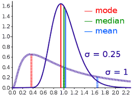
But it is not the only measure of average. Another important measure of average is the median. If you put all the data point values in order from lowest to highest then the median is the value directly in the middle, that is, it is the value for which half the data points lie below and half lie above.
Since critical decisions are often made based on knowledge only of the average of some key value, it is important to understand the extent to which the mean and median can differ for the same data. Take a look at Figure 2.21. This shows the percentage distribution of salaries (in \$) for workers in one city.
Note that the vast majority of the population (83\%) have salaries within a fairly narrow range $(\$ 10,000-\$ 50,000)$. But $2 \%$ have salaries in excess of $\$ 1$ million. The effect of this asymmetry in the distribution is that the median salary is $\$ 23,000$, whereas the mean is $\$ 137,000$. By definition half of the population earn at least the median salary; but just $5 \%$ of the population earn at least the mean salary.
Of course, the explanation for this massive difference is the “long tail” of the distribution. A small number of very high earners massively skew the mean figure. Nevertheless, for readers brought up on the notion that most data is inherently bell-shaped (i.e. a Normal distribution in the sense explained in Section 2.1) this difference between the mean and median will come as a surprise. In Normal distributions the mean and median are always equal, and in those cases you do not therefore need to worry about how you measure average.
The ramifications in decision making of failing to understand the difference between different measures of average can be devastating.
贝叶斯分析代考
统计代写|贝叶斯分析代写Bayesian Analysis代考|The Danger of Averages
弗雷德和简在两年时间里学习了同一门课程。要完成课程,他们必须完成 10 个模块。最后,他们的年均结果如表2.7所示。简的成绩每年都比弗雷德差。那么,简怎么可能获得成绩最好的学生的奖品呢?这是因为总体平均数是年度平均数的平均数,而不是所有 10 个模块的平均数。除非我们知道每个学生每年学习多少个模块,否则我们无法计算出这 10 个模块的平均值。
实际上:
- Fred 在第 1 年学习了 7 个模块,在第 2 年学习了 3 个模块
- Jane 在第 1 年选修了 2 个模块,在第 2 年选修了 8 个模块。
假设每个模块都被标记为满分 100,我们可以使用此信息来计算总分,如表 2.8 所示。很明显,简总体上比弗雷德做得更好。
这是辛普森悖论的一个例子。这似乎是一个悖论 Fred 的平均分一直高于 Jane 的平均分,但 Jane 的总体平均分更高。但这并不是真正的悖论。假设您可以在不考虑(在这种情况下)构成每个平均值的模块数量的情况下取平均数,这是完全错误的。
从下面的角度来看,一切都会变得清晰起来:在 Fred 完成大部分模块的那一年,他的平均得分为 50;在简完成大部分模块的那一年,她的平均成绩为 62 分。当你以这种方式看待它时,简的整体表现更好就不足为奇了。
这种辛普森悖论的例子在医学研究中尤为常见。考虑表 2.9-2.11 中显示的示例(基于 Bishop 等人,1975 年描述的一项研究的简化版本),其中来自许多诊所的总体汇总数据(表 2.9)的指示表明两者之间存在正相关产前护理和婴儿存活率。然而,当对每个诊所的数据进行分析时(表 2.10-2.11),在每个案例中提供产前护理时,存活率实际上较低。主教等。总结道:
“如果我们查看这张 [组合] 表,我们会错误地得出结论,认为生存与接受的护理量有关。”
统计代写|贝叶斯分析代写Bayesian Analysis代考|What Type of Average?
当我们对上面的考试分数数据使用平均值时,我们实际上使用了一种特定的(最常用的)平均值度量:平均值。这被定义为所有数据点值的总和除以数据点的数量。
但这并不是平均水平的唯一衡量标准。平均数的另一个重要衡量标准是中位数。如果将所有数据点值按从低到高的顺序排列,则中位数就是正中间的值,也就是说,它是一半数据点在下方,一半在上方的值。
由于关键决策通常仅基于对某些关键值的平均值的了解,因此了解相同数据的均值和中值的差异程度非常重要。看一下图 2.21。这显示了一个城市中工人的工资(以$ 为单位)的百分比分布。
请注意,绝大多数人 (83\%) 的薪水都在相当狭窄的范围内($10,000−$50,000). 但2%工资超过$1百万。这种分布不对称的影响是工资中位数是$23,000, 而平均值是$137,000. 根据定义,一半的人口至少赚取中位数工资;只是5%的人口至少赚取平均工资。
当然,造成这种巨大差异的原因是分布的“长尾”。少数非常高的收入者极大地扭曲了平均数字。然而,对于提出大多数数据本质上是钟形(即第 2.1 节中解释的正态分布)这一概念的读者来说,均值和中位数之间的这种差异会令人惊讶。在正态分布中,均值和中位数总是相等的,因此在这种情况下,您无需担心如何衡量平均值。
未能理解不同平均值测量之间的差异在决策过程中的后果可能是毁灭性的。

统计代写请认准statistics-lab™. statistics-lab™为您的留学生涯保驾护航。
金融工程代写
金融工程是使用数学技术来解决金融问题。金融工程使用计算机科学、统计学、经济学和应用数学领域的工具和知识来解决当前的金融问题,以及设计新的和创新的金融产品。
非参数统计代写
非参数统计指的是一种统计方法,其中不假设数据来自于由少数参数决定的规定模型;这种模型的例子包括正态分布模型和线性回归模型。
广义线性模型代考
广义线性模型(GLM)归属统计学领域,是一种应用灵活的线性回归模型。该模型允许因变量的偏差分布有除了正态分布之外的其它分布。
术语 广义线性模型(GLM)通常是指给定连续和/或分类预测因素的连续响应变量的常规线性回归模型。它包括多元线性回归,以及方差分析和方差分析(仅含固定效应)。
有限元方法代写
有限元方法(FEM)是一种流行的方法,用于数值解决工程和数学建模中出现的微分方程。典型的问题领域包括结构分析、传热、流体流动、质量运输和电磁势等传统领域。
有限元是一种通用的数值方法,用于解决两个或三个空间变量的偏微分方程(即一些边界值问题)。为了解决一个问题,有限元将一个大系统细分为更小、更简单的部分,称为有限元。这是通过在空间维度上的特定空间离散化来实现的,它是通过构建对象的网格来实现的:用于求解的数值域,它有有限数量的点。边界值问题的有限元方法表述最终导致一个代数方程组。该方法在域上对未知函数进行逼近。[1] 然后将模拟这些有限元的简单方程组合成一个更大的方程系统,以模拟整个问题。然后,有限元通过变化微积分使相关的误差函数最小化来逼近一个解决方案。
tatistics-lab作为专业的留学生服务机构,多年来已为美国、英国、加拿大、澳洲等留学热门地的学生提供专业的学术服务,包括但不限于Essay代写,Assignment代写,Dissertation代写,Report代写,小组作业代写,Proposal代写,Paper代写,Presentation代写,计算机作业代写,论文修改和润色,网课代做,exam代考等等。写作范围涵盖高中,本科,研究生等海外留学全阶段,辐射金融,经济学,会计学,审计学,管理学等全球99%专业科目。写作团队既有专业英语母语作者,也有海外名校硕博留学生,每位写作老师都拥有过硬的语言能力,专业的学科背景和学术写作经验。我们承诺100%原创,100%专业,100%准时,100%满意。
随机分析代写
随机微积分是数学的一个分支,对随机过程进行操作。它允许为随机过程的积分定义一个关于随机过程的一致的积分理论。这个领域是由日本数学家伊藤清在第二次世界大战期间创建并开始的。
时间序列分析代写
随机过程,是依赖于参数的一组随机变量的全体,参数通常是时间。 随机变量是随机现象的数量表现,其时间序列是一组按照时间发生先后顺序进行排列的数据点序列。通常一组时间序列的时间间隔为一恒定值(如1秒,5分钟,12小时,7天,1年),因此时间序列可以作为离散时间数据进行分析处理。研究时间序列数据的意义在于现实中,往往需要研究某个事物其随时间发展变化的规律。这就需要通过研究该事物过去发展的历史记录,以得到其自身发展的规律。
回归分析代写
多元回归分析渐进(Multiple Regression Analysis Asymptotics)属于计量经济学领域,主要是一种数学上的统计分析方法,可以分析复杂情况下各影响因素的数学关系,在自然科学、社会和经济学等多个领域内应用广泛。
MATLAB代写
MATLAB 是一种用于技术计算的高性能语言。它将计算、可视化和编程集成在一个易于使用的环境中,其中问题和解决方案以熟悉的数学符号表示。典型用途包括:数学和计算算法开发建模、仿真和原型制作数据分析、探索和可视化科学和工程图形应用程序开发,包括图形用户界面构建MATLAB 是一个交互式系统,其基本数据元素是一个不需要维度的数组。这使您可以解决许多技术计算问题,尤其是那些具有矩阵和向量公式的问题,而只需用 C 或 Fortran 等标量非交互式语言编写程序所需的时间的一小部分。MATLAB 名称代表矩阵实验室。MATLAB 最初的编写目的是提供对由 LINPACK 和 EISPACK 项目开发的矩阵软件的轻松访问,这两个项目共同代表了矩阵计算软件的最新技术。MATLAB 经过多年的发展,得到了许多用户的投入。在大学环境中,它是数学、工程和科学入门和高级课程的标准教学工具。在工业领域,MATLAB 是高效研究、开发和分析的首选工具。MATLAB 具有一系列称为工具箱的特定于应用程序的解决方案。对于大多数 MATLAB 用户来说非常重要,工具箱允许您学习和应用专业技术。工具箱是 MATLAB 函数(M 文件)的综合集合,可扩展 MATLAB 环境以解决特定类别的问题。可用工具箱的领域包括信号处理、控制系统、神经网络、模糊逻辑、小波、仿真等。