标签: BSTA5014

统计代写|贝叶斯分析代写Bayesian Analysis代考|MAST90125

如果你也在 怎样代写贝叶斯分析Bayesian Analysis 这个学科遇到相关的难题,请随时右上角联系我们的24/7代写客服。贝叶斯分析Bayesian Analysis是一种统计范式,它使用概率陈述来回答关于未知参数的研究问题。

贝叶斯分析Bayesian Analysis的独特特征包括能够将先验信息纳入分析,将可信区间直观地解释为固定范围,其中参数已知属于预先指定的概率,以及将实际概率分配给任何感兴趣的假设的能力。贝叶斯推断使用后验分布来形成模型参数的各种总结,包括点估计,如后验均值、中位数、百分位数和称为可信区间的区间估计。此外,所有关于模型参数的统计检验都可以表示为基于估计的后验分布的概率陈述。

statistics-lab™ 为您的留学生涯保驾护航 在代写贝叶斯分析Bayesian Analysis方面已经树立了自己的口碑, 保证靠谱, 高质且原创的统计Statistics代写服务。我们的专家在代写贝叶斯分析Bayesian Analysis代写方面经验极为丰富,各种代写贝叶斯分析Bayesian Analysis相关的作业也就用不着说。

统计代写|贝叶斯分析代写Bayesian Analysis代考|MAST90125

统计代写|贝叶斯分析代写Bayesian Analysis代考|Posterior predictive distribution for a future observation

The posterior predictive distribution for a future observation, $\tilde{y}$, can be written as a mixture, $p(\tilde{y} \mid y)=\iint p\left(\tilde{y} \mid \mu, \sigma^2, y\right) p\left(\mu, \sigma^2 \mid y\right) d \mu d \sigma^2$. The first of the two factors in the integral is just the normal distribution for the future observation given the values of $\left(\mu, \sigma^2\right)$, and does not depend on $y$ at all. To draw from the posterior predictive distribution, first draw $\mu, \sigma^2$ from their joint posterior distribution and then simulate $\tilde{y} \sim \mathrm{N}\left(\mu, \sigma^2\right)$.

In fact, the posterior predictive distribution of $\tilde{y}$ is a $t$ distribution with location $\bar{y}$, scale $\left(1+\frac{1}{n}\right)^{1 / 2} s$, and $n-1$ degrees of freedom. This analytic form is obtained using the same techniques as in the derivation of the posterior distribution of $\mu$. Specifically, the distribution can be obtained by integrating out the parameters $\mu, \sigma^2$ according to their joint posterior distribution. We can identify the result more easily by noticing that the factorization $p\left(\tilde{y} \mid \sigma^2, y\right)=\int p\left(\tilde{y} \mid \mu, \sigma^2, y\right) p\left(\mu \mid \sigma^2, y\right) d \mu$ leads to $p\left(\tilde{y} \mid \sigma^2, y\right)=\mathrm{N}\left(\tilde{y} \mid \bar{y},\left(1+\frac{1}{n}\right) \sigma^2\right)$, which is the same, up to a changed scale factor, as the distribution of $\mu \mid \sigma^2, y$.
Example. Estimating the speed of light
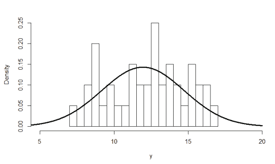
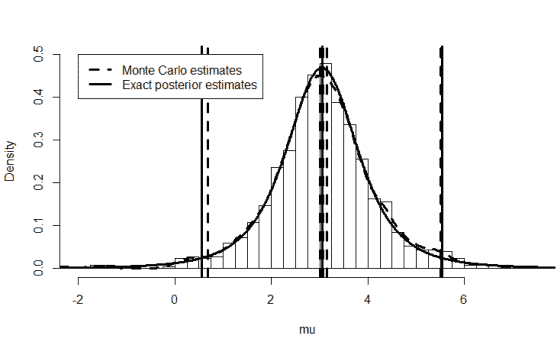
Simon Newcomb set up an experiment in 1882 to measure the speed of light. Newcomb measured the amount of time required for light to travel a distance of 7442 meters. A histogram of Newcomb’s 66 measurements is shown in Figure 3.1. There are two unusually low measurements and then a cluster of measurements that are approximately symmetrically distributed. We (inappropriately) apply the normal model, assuming that all 66 measurements are independent draws from a normal distribution with mean $\mu$ and variance $\sigma^2$. The main substantive goal is posterior inference for $\mu$. The outlying measurements do not fit the normal model; we discuss Bayesian methods for measuring the lack of fit for these data in Section 6.3. The mean of the 66 measurements is $\bar{y}=26.2$, and the sample standard deviation is $s=10.8$. Assuming the noninformative prior distribution $p\left(\mu, \sigma^2\right) \propto\left(\sigma^2\right)^{-1}$, a $95 \%$ central posterior interval for $\mu$ is obtained from the $t_{65}$ marginal posterior distribution of $\mu$ as $\bar{y} \pm 1.997 \mathrm{~s} / \sqrt{66}=[23.6,28.8]$. The posterior interval can also be obtained by simulation. Following the factorization of the posterior distribution given by (3.5) and (3.3), we first draw a random value of $\sigma^2 \sim \operatorname{Inv}-\chi^2\left(65, s^2\right)$ as $65 s^2$ divided by a random draw from the $\chi_{65}^2$ distribution (see Appendix A). Then given this value of $\sigma^2$, we draw $\mu$ from its conditional posterior distribution, $\mathrm{N}\left(26.2, \sigma^2 / 66\right)$. Based on 1000 simulated values of $\left(\mu, \sigma^2\right)$, we estimate the posterior median of $\mu$ to be 26.2 and a $95 \%$ central posterior interval for $\mu$ to be $[23.6,28.9]$, close to the analytically calculated interval.
Incidentally, based on the currently accepted value of the speed of light, the ‘true value’ for $\mu$ in Newcomb’s experiment is 33.0, which falls outside our $95 \%$ interval. This reinforces the fact that posterior inferences are only as good as the model and the experiment that produced the data.

统计代写|贝叶斯分析代写Bayesian Analysis代考|Normal data with a conjugate prior distribution

A first step toward a more general model is to assume a conjugate prior distribution for the two-parameter univariate normal sampling model in place of the noninformative prior distribution just considered. The form of the likelihood displayed in (3.2) and the subsequent discussion shows that the conjugate prior density must also have the product form $p\left(\sigma^2\right) p\left(\mu \mid \sigma^2\right)$, where the marginal distribution of $\sigma^2$ is scaled inverse- $\chi^2$ and the conditional distribution of $\mu$ given $\sigma^2$ is normal (so that marginally $\mu$ has a $t$ distribution). A convenient parameterization is given by the following specification:
$$
\begin{aligned}
\mu \mid \sigma^2 & \sim \mathrm{N}\left(\mu_0, \sigma^2 / \kappa_0\right) \
\sigma^2 & \sim \operatorname{Inv}-\chi^2\left(\nu_0, \sigma_0^2\right),
\end{aligned}
$$
which corresponds to the joint prior density
$$
p\left(\mu, \sigma^2\right) \propto \sigma^{-1}\left(\sigma^2\right)^{-\left(\nu_0 / 2+1\right)} \exp \left(-\frac{1}{2 \sigma^2}\left[\nu_0 \sigma_0^2+\kappa_0\left(\mu_0-\mu\right)^2\right]\right) .
$$
We label this the N-Inv- $\chi^2\left(\mu_0, \sigma_0^2 / \kappa_0 ; \nu_0, \sigma_0^2\right)$ density; its four parameters can be identified as the location and scale of $\mu$ and the degrees of freedom and scale of $\sigma^2$, respectively.

The appearance of $\sigma^2$ in the conditional distribution of $\mu \mid \sigma^2$ means that $\mu$ and $\sigma^2$ are necessarily dependent in their joint conjugate prior density: for example, if $\sigma^2$ is large, then a high-variance prior distribution is induced on $\mu$. This dependence is notable, considering that conjugate prior distributions are used largely for convenience. Upon reflection, however, it often makes sense for the prior variance of the mean to be tied to $\sigma^2$, which is the sampling variance of the observation $y$. In this way, prior belief about $\mu$ is calibrated by the scale of measurement of $y$ and is equivalent to $\kappa_0$ prior measurements on this scale.

统计代写|贝叶斯分析代写Bayesian Analysis代考|MAST90125

贝叶斯分析代考

统计代写|贝叶斯分析代写Bayesian Analysis代考|Posterior predictive distribution for a future observation

一个未来观测值$\tilde{y}$的后验预测分布可以写成一个混合物$p(\tilde{y} \mid y)=\iint p\left(\tilde{y} \mid \mu, \sigma^2, y\right) p\left(\mu, \sigma^2 \mid y\right) d \mu d \sigma^2$。积分中两个因子中的第一个是给定$\left(\mu, \sigma^2\right)$值的未来观测值的正态分布,完全不依赖于$y$。要从后验预测分布中提取,首先从它们的联合后验分布中提取$\mu, \sigma^2$,然后模拟$\tilde{y} \sim \mathrm{N}\left(\mu, \sigma^2\right)$。

事实上,$\tilde{y}$的后验预测分布是一个$t$分布,其位置为$\bar{y}$,规模为$\left(1+\frac{1}{n}\right)^{1 / 2} s$,自由度为$n-1$。这种解析形式是使用与推导$\mu$后验分布相同的技术得到的。具体来说,可以根据参数$\mu, \sigma^2$的关节后验分布积分得到其分布。我们可以更容易地识别结果,注意到分解$p\left(\tilde{y} \mid \sigma^2, y\right)=\int p\left(\tilde{y} \mid \mu, \sigma^2, y\right) p\left(\mu \mid \sigma^2, y\right) d \mu$导致$p\left(\tilde{y} \mid \sigma^2, y\right)=\mathrm{N}\left(\tilde{y} \mid \bar{y},\left(1+\frac{1}{n}\right) \sigma^2\right)$,它与$\mu \mid \sigma^2, y$的分布相同,直到改变了比例因子。
示例:估计光速
西蒙·纽科姆在1882年建立了一个测量光速的实验。纽科姆测量了光传播7442米所需的时间。Newcomb的66次测量的直方图如图3.1所示。有两个异常低的测量值,然后是一组近似对称分布的测量值。我们(不恰当地)应用正态模型,假设所有66个测量值都是独立的,来自均值$\mu$和方差$\sigma^2$的正态分布。主要的实质性目标是$\mu$的后验推理。外围测量值不符合正态模型;我们将在第6.3节讨论贝叶斯方法来测量这些数据的拟合缺失。66次测量的平均值为$\bar{y}=26.2$,样本标准差为$s=10.8$。假设无信息先验分布$p\left(\mu, \sigma^2\right) \propto\left(\sigma^2\right)^{-1}$,由$\mu$的边际后验分布$t_{65}$得到$\mu$的中心后验区间$95 \%$为$\bar{y} \pm 1.997 \mathrm{~s} / \sqrt{66}=[23.6,28.8]$。后验区间也可以通过仿真得到。根据(3.5)和(3.3)给出的后验分布的因式分解,我们首先得出一个随机值$\sigma^2 \sim \operatorname{Inv}-\chi^2\left(65, s^2\right)$,即$65 s^2$除以$\chi_{65}^2$分布的随机值(见附录a)。然后给出这个值$\sigma^2$,我们从它的条件后验分布$\mathrm{N}\left(26.2, \sigma^2 / 66\right)$中得出$\mu$。基于$\left(\mu, \sigma^2\right)$的1000个模拟值,我们估计$\mu$的后验中位数为26.2,$\mu$的$95 \%$中央后验区间为$[23.6,28.9]$,接近解析计算的区间。
顺便说一句,根据目前公认的光速值,纽科姆实验中$\mu$的“真实值”是33.0,这超出了我们的$95 \%$区间。这强化了一个事实,即后验推断只与产生数据的模型和实验一样好。

统计代写|贝叶斯分析代写Bayesian Analysis代考|Normal data with a conjugate prior distribution

建立更一般模型的第一步是假设双参数单变量正态抽样模型的共轭先验分布取代刚才考虑的非信息先验分布。(3.2)中显示的似然形式和随后的讨论表明,共轭先验密度也必须具有乘积形式$p\left(\sigma^2\right) p\left(\mu \mid \sigma^2\right)$,其中$\sigma^2$的边际分布按比例为逆- $\chi^2$,并且$\mu$给定$\sigma^2$的条件分布为正态分布(因此边际$\mu$具有$t$分布)。下面的规范给出了一个方便的参数化:
$$
\begin{aligned}
\mu \mid \sigma^2 & \sim \mathrm{N}\left(\mu_0, \sigma^2 / \kappa_0\right) \
\sigma^2 & \sim \operatorname{Inv}-\chi^2\left(\nu_0, \sigma_0^2\right),
\end{aligned}
$$
哪个对应于关节先验密度
$$
p\left(\mu, \sigma^2\right) \propto \sigma^{-1}\left(\sigma^2\right)^{-\left(\nu_0 / 2+1\right)} \exp \left(-\frac{1}{2 \sigma^2}\left[\nu_0 \sigma_0^2+\kappa_0\left(\mu_0-\mu\right)^2\right]\right) .
$$
我们把它标记为N-Inv- $\chi^2\left(\mu_0, \sigma_0^2 / \kappa_0 ; \nu_0, \sigma_0^2\right)$密度;它的四个参数分别可以识别为$\mu$的位置和尺度以及$\sigma^2$的自由度和尺度。

$\sigma^2$在$\mu \mid \sigma^2$的条件分布中的出现意味着$\mu$和$\sigma^2$在它们的联合共轭先验密度上是必然依赖的:例如,如果$\sigma^2$很大,那么在$\mu$上就会产生一个高方差先验分布。考虑到共轭先验分布主要是为了方便而使用,这种依赖性是值得注意的。然而,经过反思,通常将均值的先验方差与$\sigma^2$联系起来是有意义的,这是观测值的抽样方差$y$。这样,关于$\mu$的先验信念是通过$y$的测量尺度来校准的,相当于$\kappa_0$在这个尺度上的先验测量。

统计代写|贝叶斯分析代写Bayesian Analysis代考 请认准statistics-lab™

统计代写请认准statistics-lab™. statistics-lab™为您的留学生涯保驾护航。

金融工程代写

金融工程是使用数学技术来解决金融问题。金融工程使用计算机科学、统计学、经济学和应用数学领域的工具和知识来解决当前的金融问题,以及设计新的和创新的金融产品。

非参数统计代写

非参数统计指的是一种统计方法,其中不假设数据来自于由少数参数决定的规定模型;这种模型的例子包括正态分布模型和线性回归模型。

广义线性模型代考

广义线性模型(GLM)归属统计学领域,是一种应用灵活的线性回归模型。该模型允许因变量的偏差分布有除了正态分布之外的其它分布。

术语 广义线性模型(GLM)通常是指给定连续和/或分类预测因素的连续响应变量的常规线性回归模型。它包括多元线性回归,以及方差分析和方差分析(仅含固定效应)。

有限元方法代写

有限元方法(FEM)是一种流行的方法,用于数值解决工程和数学建模中出现的微分方程。典型的问题领域包括结构分析、传热、流体流动、质量运输和电磁势等传统领域。

有限元是一种通用的数值方法,用于解决两个或三个空间变量的偏微分方程(即一些边界值问题)。为了解决一个问题,有限元将一个大系统细分为更小、更简单的部分,称为有限元。这是通过在空间维度上的特定空间离散化来实现的,它是通过构建对象的网格来实现的:用于求解的数值域,它有有限数量的点。边界值问题的有限元方法表述最终导致一个代数方程组。该方法在域上对未知函数进行逼近。[1] 然后将模拟这些有限元的简单方程组合成一个更大的方程系统,以模拟整个问题。然后,有限元通过变化微积分使相关的误差函数最小化来逼近一个解决方案。

tatistics-lab作为专业的留学生服务机构,多年来已为美国、英国、加拿大、澳洲等留学热门地的学生提供专业的学术服务,包括但不限于Essay代写,Assignment代写,Dissertation代写,Report代写,小组作业代写,Proposal代写,Paper代写,Presentation代写,计算机作业代写,论文修改和润色,网课代做,exam代考等等。写作范围涵盖高中,本科,研究生等海外留学全阶段,辐射金融,经济学,会计学,审计学,管理学等全球99%专业科目。写作团队既有专业英语母语作者,也有海外名校硕博留学生,每位写作老师都拥有过硬的语言能力,专业的学科背景和学术写作经验。我们承诺100%原创,100%专业,100%准时,100%满意。

随机分析代写


随机微积分是数学的一个分支,对随机过程进行操作。它允许为随机过程的积分定义一个关于随机过程的一致的积分理论。这个领域是由日本数学家伊藤清在第二次世界大战期间创建并开始的。

时间序列分析代写

随机过程,是依赖于参数的一组随机变量的全体,参数通常是时间。 随机变量是随机现象的数量表现,其时间序列是一组按照时间发生先后顺序进行排列的数据点序列。通常一组时间序列的时间间隔为一恒定值(如1秒,5分钟,12小时,7天,1年),因此时间序列可以作为离散时间数据进行分析处理。研究时间序列数据的意义在于现实中,往往需要研究某个事物其随时间发展变化的规律。这就需要通过研究该事物过去发展的历史记录,以得到其自身发展的规律。

回归分析代写

多元回归分析渐进(Multiple Regression Analysis Asymptotics)属于计量经济学领域,主要是一种数学上的统计分析方法,可以分析复杂情况下各影响因素的数学关系,在自然科学、社会和经济学等多个领域内应用广泛。

MATLAB代写

MATLAB 是一种用于技术计算的高性能语言。它将计算、可视化和编程集成在一个易于使用的环境中,其中问题和解决方案以熟悉的数学符号表示。典型用途包括:数学和计算算法开发建模、仿真和原型制作数据分析、探索和可视化科学和工程图形应用程序开发,包括图形用户界面构建MATLAB 是一个交互式系统,其基本数据元素是一个不需要维度的数组。这使您可以解决许多技术计算问题,尤其是那些具有矩阵和向量公式的问题,而只需用 C 或 Fortran 等标量非交互式语言编写程序所需的时间的一小部分。MATLAB 名称代表矩阵实验室。MATLAB 最初的编写目的是提供对由 LINPACK 和 EISPACK 项目开发的矩阵软件的轻松访问,这两个项目共同代表了矩阵计算软件的最新技术。MATLAB 经过多年的发展,得到了许多用户的投入。在大学环境中,它是数学、工程和科学入门和高级课程的标准教学工具。在工业领域,MATLAB 是高效研究、开发和分析的首选工具。MATLAB 具有一系列称为工具箱的特定于应用程序的解决方案。对于大多数 MATLAB 用户来说非常重要,工具箱允许您学习应用专业技术。工具箱是 MATLAB 函数(M 文件)的综合集合,可扩展 MATLAB 环境以解决特定类别的问题。可用工具箱的领域包括信号处理、控制系统、神经网络、模糊逻辑、小波、仿真等。

R语言代写问卷设计与分析代写
PYTHON代写回归分析与线性模型代写
MATLAB代写方差分析与试验设计代写
STATA代写机器学习/统计学习代写
SPSS代写计量经济学代写
EVIEWS代写时间序列分析代写
EXCEL代写深度学习代写
SQL代写各种数据建模与可视化代写

统计代写|贝叶斯分析代写Bayesian Analysis代考|P-533

如果你也在 怎样代写贝叶斯分析Bayesian Analysis 这个学科遇到相关的难题,请随时右上角联系我们的24/7代写客服。贝叶斯分析Bayesian Analysis是一种统计范式,它使用概率陈述来回答关于未知参数的研究问题。

贝叶斯分析Bayesian Analysis的独特特征包括能够将先验信息纳入分析,将可信区间直观地解释为固定范围,其中参数已知属于预先指定的概率,以及将实际概率分配给任何感兴趣的假设的能力。贝叶斯推断使用后验分布来形成模型参数的各种总结,包括点估计,如后验均值、中位数、百分位数和称为可信区间的区间估计。此外,所有关于模型参数的统计检验都可以表示为基于估计的后验分布的概率陈述。

statistics-lab™ 为您的留学生涯保驾护航 在代写贝叶斯分析Bayesian Analysis方面已经树立了自己的口碑, 保证靠谱, 高质且原创的统计Statistics代写服务。我们的专家在代写贝叶斯分析Bayesian Analysis代写方面经验极为丰富,各种代写贝叶斯分析Bayesian Analysis相关的作业也就用不着说。

统计代写|贝叶斯分析代写Bayesian Analysis代考|P-533

统计代写|贝叶斯分析代写Bayesian Analysis代考|Constructing a weakly informative prior distribution

One might argue that virtually all statistical models are weakly informative: a model always conveys some information, if only in its choice of inputs and the functional form of how they are combined, but it is not possible or perhaps even desirable to encode all of one’s prior beliefs about a subject into a set of probability distributions. With that in mind, we offer two principles for setting up weakly informative priors, going at the problem from two different directions:

  • Start with some version of a noninformative prior distribution and then add enough information so that inferences are constrained to be reasonable.
  • Start with a strong, highly informative prior and broaden it to account for uncertainty in one’s prior beliefs and in the applicability of any historically based prior distribution to new data.

Neither of these approaches is pure. In the first case, it can happen that the purportedly noninformative prior distribution used as a starting point is in fact too strong. For example, if a $\mathrm{U}(0,1)$ prior distribution is assigned to the probability of some rare disease, then in the presence of weak data the probability can be grossly overestimated (suppose $y=0$ incidences out of $n=100$ cases, and the true prevalence is known to be less than 1 in $10,000)$, and an appropriate weakly informative prior will be such that the posterior in this case will be concentrated in that low range. In the second case, a prior distribution that is believed to be strongly informative may in fact be too weak along some direction. This is not to say that priors should be made more precise whenever posterior inferences are vague; in many cases, our best strategy is simply to acknowledge whatever posterior uncertainty we have. But we should not feel constrained by default noninformative models when we have substantive prior knowledge available.

统计代写|贝叶斯分析代写Bayesian Analysis代考|Bibliographic note

A fascinating detailed account of the early development of the idea of ‘inverse probability’ (Bayesian inference) is provided in the book by Stigler (1986), on which our brief accounts of Bayes’ and Laplace’s solutions to the problem of estimating an unknown proportion are based. Bayes’ famous 1763 essay in the Philosophical Transactions of the Royal Society of London has been reprinted as Bayes (1763); see also Laplace $(1785,1810)$.

Introductory textbooks providing complementary discussions of the simple models covered in this chapter were listed at the end of Chapter 1. In particular, Box and Tiao (1973) provide a detailed treatment of Bayesian analysis with the normal model and also discuss highest posterior density regions in some detail. The theory of conjugate prior distributions was developed in detail by Raiffa and Schlaifer (1961). An interesting account of inference for prediction, which also includes extensive details of particular probability models and conjugate prior analyses, appears in Aitchison and Dunsmore (1975).

Liu et al. (2013) discuss how to efficiently compute highest posterior density intervals using simulations.

Noninformative and reference prior distributions have been studied by many researchers. Jeffreys (1961) and Hartigan (1964) discuss invariance principles for noninformative prior distributions. Chapter 1 of Box and Tiao (1973) presents a straightforward and practically oriented discussion, a brief but detailed survey is given by Berger (1985), and the article by Bernardo (1979) is accompanied by a wide-ranging discussion. Bernardo and Smith (1994) give an extensive treatment of this topic along with many other matters relevant to the construction of prior distributions. Barnard (1985) discusses the relation between pivotal quantities and noninformative Bayesian inference. Kass and Wasserman (1996) provide a review of many approaches for establishing noninformative prior densities based on Jeffreys’ rule, and they also discuss the problems that may arise from uncritical use of purportedly noninformative prior specifications. Dawid, Stone, and Zidek (1973) discuss some difficulties that can arise with noninformative prior distributions; also see Jaynes (1980).

统计代写|贝叶斯分析代写Bayesian Analysis代考|P-533

贝叶斯分析代考

统计代写|贝叶斯分析代写Bayesian Analysis代考|Constructing a weakly informative prior distribution

有人可能会争辩说,实际上所有的统计模型都是弱信息性的:一个模型总是传达一些信息,如果只是在输入的选择和它们如何组合的功能形式中,但是将一个人对一个主题的所有先验信念编码成一组概率分布是不可能的,甚至是不可取的。考虑到这一点,我们提供了建立弱信息先验的两个原则,从两个不同的方向来解决问题:

从非信息性先验分布的某个版本开始,然后添加足够的信息,这样推理就会被限制在合理的范围内。

从一个强大的、信息丰富的先验开始,并将其扩展到一个人的先验信念中的不确定性,以及任何基于历史的先验分布对新数据的适用性。

这两种方法都不是纯粹的。在第一种情况下,作为起点的所谓无信息先验分布实际上过于强大。例如,如果将一个$\ mathm {U}(0,1)$先验分布分配给某些罕见疾病的概率,那么在存在弱数据的情况下,概率可能会被严重高估(假设$y=0$发病率在$n=100$病例中,并且已知真实患病率小于1 / 10,000 $)$,并且适当的弱信息先验将使得这种情况下的后验将集中在那个低范围内。在第二种情况下,被认为信息量很强的先验分布实际上可能在某些方向上太弱。这并不是说,当后验推理模糊不清时,先验就应该更精确;在很多情况下,我们最好的策略就是承认我们所拥有的后验不确定性。但是,当我们有实质性的先验知识可用时,我们不应该被默认的非信息模型所约束。

统计代写|贝叶斯分析代写Bayesian Analysis代考|Bibliographic note

Stigler(1986)的书中提供了“逆概率”(贝叶斯推理)概念早期发展的迷人详细描述,我们对贝叶斯和拉普拉斯估计未知比例问题的解决方案的简要说明是基于此的。贝叶斯1763年在《伦敦皇家学会哲学会刊》上发表的著名文章已被重印为贝叶斯(1763);另见拉普拉斯$(1785,1810)$。

提供本章所涵盖的简单模型的补充讨论的介绍性教科书在第1章末尾列出。特别是Box和Tiao(1973)用正态模型对贝叶斯分析进行了详细的处理,并对最高后验密度区域进行了详细的讨论。共轭先验分布理论是由Raiffa和Schlaifer(1961)详细发展起来的。在Aitchison和Dunsmore(1975)中,有一个关于预测推理的有趣描述,其中还包括特定概率模型和共轭先验分析的广泛细节。

Liu等人(2013)讨论了如何使用模拟有效地计算最高后验密度间隔。

非信息先验分布和参考先验分布已经被许多研究者研究过。Jeffreys(1961)和Hartigan(1964)讨论了非信息性先验分布的不变性原则。Box and Tiao(1973)的第一章提出了一个直截了当的和实际导向的讨论,Berger(1985)给出了一个简短但详细的调查,Bernardo(1979)的文章伴随着一个广泛的讨论。Bernardo和Smith(1994)对这一主题以及与先验分布的构建相关的许多其他问题进行了广泛的处理。Barnard(1985)讨论了关键量和非信息贝叶斯推理之间的关系。Kass和Wasserman(1996)对基于Jeffreys规则建立非信息先验密度的许多方法进行了回顾,他们还讨论了不加批判地使用所谓的非信息先验规范可能产生的问题。david, Stone和Zidek(1973)讨论了非信息性先验分布可能出现的一些困难;参见Jaynes(1980)。

统计代写|贝叶斯分析代写Bayesian Analysis代考 请认准statistics-lab™

统计代写请认准statistics-lab™. statistics-lab™为您的留学生涯保驾护航。

金融工程代写

金融工程是使用数学技术来解决金融问题。金融工程使用计算机科学、统计学、经济学和应用数学领域的工具和知识来解决当前的金融问题,以及设计新的和创新的金融产品。

非参数统计代写

非参数统计指的是一种统计方法,其中不假设数据来自于由少数参数决定的规定模型;这种模型的例子包括正态分布模型和线性回归模型。

广义线性模型代考

广义线性模型(GLM)归属统计学领域,是一种应用灵活的线性回归模型。该模型允许因变量的偏差分布有除了正态分布之外的其它分布。

术语 广义线性模型(GLM)通常是指给定连续和/或分类预测因素的连续响应变量的常规线性回归模型。它包括多元线性回归,以及方差分析和方差分析(仅含固定效应)。

有限元方法代写

有限元方法(FEM)是一种流行的方法,用于数值解决工程和数学建模中出现的微分方程。典型的问题领域包括结构分析、传热、流体流动、质量运输和电磁势等传统领域。

有限元是一种通用的数值方法,用于解决两个或三个空间变量的偏微分方程(即一些边界值问题)。为了解决一个问题,有限元将一个大系统细分为更小、更简单的部分,称为有限元。这是通过在空间维度上的特定空间离散化来实现的,它是通过构建对象的网格来实现的:用于求解的数值域,它有有限数量的点。边界值问题的有限元方法表述最终导致一个代数方程组。该方法在域上对未知函数进行逼近。[1] 然后将模拟这些有限元的简单方程组合成一个更大的方程系统,以模拟整个问题。然后,有限元通过变化微积分使相关的误差函数最小化来逼近一个解决方案。

tatistics-lab作为专业的留学生服务机构,多年来已为美国、英国、加拿大、澳洲等留学热门地的学生提供专业的学术服务,包括但不限于Essay代写,Assignment代写,Dissertation代写,Report代写,小组作业代写,Proposal代写,Paper代写,Presentation代写,计算机作业代写,论文修改和润色,网课代做,exam代考等等。写作范围涵盖高中,本科,研究生等海外留学全阶段,辐射金融,经济学,会计学,审计学,管理学等全球99%专业科目。写作团队既有专业英语母语作者,也有海外名校硕博留学生,每位写作老师都拥有过硬的语言能力,专业的学科背景和学术写作经验。我们承诺100%原创,100%专业,100%准时,100%满意。

随机分析代写


随机微积分是数学的一个分支,对随机过程进行操作。它允许为随机过程的积分定义一个关于随机过程的一致的积分理论。这个领域是由日本数学家伊藤清在第二次世界大战期间创建并开始的。

时间序列分析代写

随机过程,是依赖于参数的一组随机变量的全体,参数通常是时间。 随机变量是随机现象的数量表现,其时间序列是一组按照时间发生先后顺序进行排列的数据点序列。通常一组时间序列的时间间隔为一恒定值(如1秒,5分钟,12小时,7天,1年),因此时间序列可以作为离散时间数据进行分析处理。研究时间序列数据的意义在于现实中,往往需要研究某个事物其随时间发展变化的规律。这就需要通过研究该事物过去发展的历史记录,以得到其自身发展的规律。

回归分析代写

多元回归分析渐进(Multiple Regression Analysis Asymptotics)属于计量经济学领域,主要是一种数学上的统计分析方法,可以分析复杂情况下各影响因素的数学关系,在自然科学、社会和经济学等多个领域内应用广泛。

MATLAB代写

MATLAB 是一种用于技术计算的高性能语言。它将计算、可视化和编程集成在一个易于使用的环境中,其中问题和解决方案以熟悉的数学符号表示。典型用途包括:数学和计算算法开发建模、仿真和原型制作数据分析、探索和可视化科学和工程图形应用程序开发,包括图形用户界面构建MATLAB 是一个交互式系统,其基本数据元素是一个不需要维度的数组。这使您可以解决许多技术计算问题,尤其是那些具有矩阵和向量公式的问题,而只需用 C 或 Fortran 等标量非交互式语言编写程序所需的时间的一小部分。MATLAB 名称代表矩阵实验室。MATLAB 最初的编写目的是提供对由 LINPACK 和 EISPACK 项目开发的矩阵软件的轻松访问,这两个项目共同代表了矩阵计算软件的最新技术。MATLAB 经过多年的发展,得到了许多用户的投入。在大学环境中,它是数学、工程和科学入门和高级课程的标准教学工具。在工业领域,MATLAB 是高效研究、开发和分析的首选工具。MATLAB 具有一系列称为工具箱的特定于应用程序的解决方案。对于大多数 MATLAB 用户来说非常重要,工具箱允许您学习应用专业技术。工具箱是 MATLAB 函数(M 文件)的综合集合,可扩展 MATLAB 环境以解决特定类别的问题。可用工具箱的领域包括信号处理、控制系统、神经网络、模糊逻辑、小波、仿真等。

R语言代写问卷设计与分析代写
PYTHON代写回归分析与线性模型代写
MATLAB代写方差分析与试验设计代写
STATA代写机器学习/统计学习代写
SPSS代写计量经济学代写
EVIEWS代写时间序列分析代写
EXCEL代写深度学习代写
SQL代写各种数据建模与可视化代写

统计代写|贝叶斯分析代写Bayesian Analysis代考|STAT3303

如果你也在 怎样代写贝叶斯分析Bayesian Analysis 这个学科遇到相关的难题,请随时右上角联系我们的24/7代写客服。贝叶斯分析Bayesian Analysis是一种统计范式,它使用概率陈述来回答关于未知参数的研究问题。

贝叶斯分析Bayesian Analysis的独特特征包括能够将先验信息纳入分析,将可信区间直观地解释为固定范围,其中参数已知属于预先指定的概率,以及将实际概率分配给任何感兴趣的假设的能力。贝叶斯推断使用后验分布来形成模型参数的各种总结,包括点估计,如后验均值、中位数、百分位数和称为可信区间的区间估计。此外,所有关于模型参数的统计检验都可以表示为基于估计的后验分布的概率陈述。

statistics-lab™ 为您的留学生涯保驾护航 在代写贝叶斯分析Bayesian Analysis方面已经树立了自己的口碑, 保证靠谱, 高质且原创的统计Statistics代写服务。我们的专家在代写贝叶斯分析Bayesian Analysis代写方面经验极为丰富,各种代写贝叶斯分析Bayesian Analysis相关的作业也就用不着说。

统计代写|贝叶斯分析代写Bayesian Analysis代考|STAT3303

统计代写|贝叶斯分析代写Bayesian Analysis代考|Other standard single-parameter models

Recall that, in general, the posterior density, $p(\theta \mid y)$, has no closed-form expression; the normalizing constant, $p(y)$, is often especially difficult to compute due to the integral (1.3). Much formal Bayesian analysis concentrates on situations where closed forms are available; such models are sometimes unrealistic, but their analysis often provides a useful starting point when it comes to constructing more realistic models.

The standard distributions – binomial, normal, Poisson, and exponential – have natural derivations from simple probability models. As we have already discussed, the binomial distribution is motivated from counting exchangeable outcomes, and the normal distribution applies to a random variable that is the sum of many exchangeable or independent terms. We will also have occasion to apply the normal distribution to the logarithm of allpositive data, which would naturally apply to observations that are modeled as the product of many independent multiplicative factors. The Poisson and exponential distributions arise as the number of counts and the waiting times, respectively, for events modeled as occurring exchangeably in all time intervals; that is, independently in time, with a constant rate of occurrence. We will generally construct realistic probability models for more complicated outcomes by combinations of these basic distributions. For example, in Section 22.2, we model the reaction times of schizophrenic patients in a psychological experiment as a binomial mixture of normal distributions on the logarithmic scale.

Each of these standard models has an associated family of conjugate prior distributions, which we discuss in turn.

统计代写|贝叶斯分析代写Bayesian Analysis代考|Normal distribution with known mean but unknown variance

The normal model with known mean $\theta$ and unknown variance is an important example, not necessarily for its direct applied value, but as a building block for more complicated, useful models, most immediately the normal distribution with unknown mean and variance, which we cover in Section 3.2. In addition, the normal distribution with known mean but unknown variance provides an introductory example of the estimation of a scale parameter.
For $p\left(y \mid \theta, \sigma^2\right)=\mathrm{N}\left(y \mid \theta, \sigma^2\right)$, with $\theta$ known and $\sigma^2$ unknown, the likelihood for a vector $y$ of $n$ independent and identically distributed observations is
$$
\begin{aligned}
p\left(y \mid \sigma^2\right) & \propto \sigma^{-n} \exp \left(-\frac{1}{2 \sigma^2} \sum_{i=1}^n\left(y_i-\theta\right)^2\right) \
& =\left(\sigma^2\right)^{-n / 2} \exp \left(-\frac{n}{2 \sigma^2} v\right) .
\end{aligned}
$$
The sufficient statistic is
$$
v=\frac{1}{n} \sum_{i=1}^n\left(y_i-\theta\right)^2 .
$$
The corresponding conjugate prior density is the inverse-gamma,
$$
p\left(\sigma^2\right) \propto\left(\sigma^2\right)^{-(\alpha+1)} e^{-\beta / \sigma^2},
$$
which has hyperparameters $(\alpha, \beta)$. A convenient parameterization is as a scaled inverse- $\chi^2$ distribution with scale $\sigma_0^2$ and $\nu_0$ degrees of freedom (see Appendix A); that is, the prior distribution of $\sigma^2$ is taken to be the distribution of $\sigma_0^2 \nu_0 / X$, where $X$ is a $\chi_{\nu_0}^2$ random variable. We use the convenient but nonstandard notation, $\sigma^2 \sim \operatorname{Inv}-\chi^2\left(\nu_0, \sigma_0^2\right)$.

统计代写|贝叶斯分析代写Bayesian Analysis代考|STAT3303

贝叶斯分析代考

统计代写|贝叶斯分析代写Bayesian Analysis代考|Other standard single-parameter models

回想一下,一般来说,后密度$p(\theta \mid y)$没有封闭形式的表达式;归一化常数$p(y)$,由于积分(1.3),通常特别难以计算。许多正式的贝叶斯分析集中在封闭形式可用的情况下;这样的模型有时是不现实的,但是当涉及到构建更现实的模型时,它们的分析通常提供了一个有用的起点。

标准分布——二项分布、正态分布、泊松分布和指数分布——可以从简单的概率模型中自然推导出来。正如我们已经讨论过的,二项分布的动机是计数可交换的结果,而正态分布适用于一个随机变量,它是许多可交换或独立项的总和。我们还将有机会将正态分布应用于所有正数据的对数,这自然适用于作为许多独立乘法因子的乘积建模的观测结果。泊松分布和指数分布分别随着计数数和等待时间的增加而出现,对于在所有时间间隔内交替发生的事件进行建模;也就是说,独立于时间,以恒定的发生速率。通过这些基本分布的组合,我们通常会为更复杂的结果构建现实的概率模型。例如,在第22.2节中,我们将心理实验中精神分裂症患者的反应时间建模为对数尺度上正态分布的二项混合。

每个标准模型都有一个相关的共轭先验分布族,我们将依次讨论。

统计代写|贝叶斯分析代写Bayesian Analysis代考|Normal distribution with known mean but unknown variance

具有已知均值$\theta$和未知方差的正态模型是一个重要的例子,不一定是因为它的直接应用价值,而是作为更复杂,有用的模型的组成部分,最直接的是具有未知均值和方差的正态分布,我们将在3.2节中介绍。此外,均值已知但方差未知的正态分布提供了一个尺度参数估计的入门示例。
对于$p\left(y \mid \theta, \sigma^2\right)=\mathrm{N}\left(y \mid \theta, \sigma^2\right)$, $\theta$已知,$\sigma^2$未知,则$n$独立且分布相同的观测值的向量$y$的可能性为
$$
\begin{aligned}
p\left(y \mid \sigma^2\right) & \propto \sigma^{-n} \exp \left(-\frac{1}{2 \sigma^2} \sum_{i=1}^n\left(y_i-\theta\right)^2\right) \
& =\left(\sigma^2\right)^{-n / 2} \exp \left(-\frac{n}{2 \sigma^2} v\right) .
\end{aligned}
$$
充分统计量为
$$
v=\frac{1}{n} \sum_{i=1}^n\left(y_i-\theta\right)^2 .
$$
对应的共轭先验密度是逆,
$$
p\left(\sigma^2\right) \propto\left(\sigma^2\right)^{-(\alpha+1)} e^{-\beta / \sigma^2},
$$
它有超参数$(\alpha, \beta)$。一种方便的参数化是一个尺度逆- $\chi^2$分布,其尺度为$\sigma_0^2$和$\nu_0$自由度(见附录A);即取$\sigma^2$的先验分布为$\sigma_0^2 \nu_0 / X$的分布,其中$X$为一个$\chi_{\nu_0}^2$随机变量。我们使用方便但不标准的符号$\sigma^2 \sim \operatorname{Inv}-\chi^2\left(\nu_0, \sigma_0^2\right)$。

统计代写|贝叶斯分析代写Bayesian Analysis代考 请认准statistics-lab™

统计代写请认准statistics-lab™. statistics-lab™为您的留学生涯保驾护航。

金融工程代写

金融工程是使用数学技术来解决金融问题。金融工程使用计算机科学、统计学、经济学和应用数学领域的工具和知识来解决当前的金融问题,以及设计新的和创新的金融产品。

非参数统计代写

非参数统计指的是一种统计方法,其中不假设数据来自于由少数参数决定的规定模型;这种模型的例子包括正态分布模型和线性回归模型。

广义线性模型代考

广义线性模型(GLM)归属统计学领域,是一种应用灵活的线性回归模型。该模型允许因变量的偏差分布有除了正态分布之外的其它分布。

术语 广义线性模型(GLM)通常是指给定连续和/或分类预测因素的连续响应变量的常规线性回归模型。它包括多元线性回归,以及方差分析和方差分析(仅含固定效应)。

有限元方法代写

有限元方法(FEM)是一种流行的方法,用于数值解决工程和数学建模中出现的微分方程。典型的问题领域包括结构分析、传热、流体流动、质量运输和电磁势等传统领域。

有限元是一种通用的数值方法,用于解决两个或三个空间变量的偏微分方程(即一些边界值问题)。为了解决一个问题,有限元将一个大系统细分为更小、更简单的部分,称为有限元。这是通过在空间维度上的特定空间离散化来实现的,它是通过构建对象的网格来实现的:用于求解的数值域,它有有限数量的点。边界值问题的有限元方法表述最终导致一个代数方程组。该方法在域上对未知函数进行逼近。[1] 然后将模拟这些有限元的简单方程组合成一个更大的方程系统,以模拟整个问题。然后,有限元通过变化微积分使相关的误差函数最小化来逼近一个解决方案。

tatistics-lab作为专业的留学生服务机构,多年来已为美国、英国、加拿大、澳洲等留学热门地的学生提供专业的学术服务,包括但不限于Essay代写,Assignment代写,Dissertation代写,Report代写,小组作业代写,Proposal代写,Paper代写,Presentation代写,计算机作业代写,论文修改和润色,网课代做,exam代考等等。写作范围涵盖高中,本科,研究生等海外留学全阶段,辐射金融,经济学,会计学,审计学,管理学等全球99%专业科目。写作团队既有专业英语母语作者,也有海外名校硕博留学生,每位写作老师都拥有过硬的语言能力,专业的学科背景和学术写作经验。我们承诺100%原创,100%专业,100%准时,100%满意。

随机分析代写


随机微积分是数学的一个分支,对随机过程进行操作。它允许为随机过程的积分定义一个关于随机过程的一致的积分理论。这个领域是由日本数学家伊藤清在第二次世界大战期间创建并开始的。

时间序列分析代写

随机过程,是依赖于参数的一组随机变量的全体,参数通常是时间。 随机变量是随机现象的数量表现,其时间序列是一组按照时间发生先后顺序进行排列的数据点序列。通常一组时间序列的时间间隔为一恒定值(如1秒,5分钟,12小时,7天,1年),因此时间序列可以作为离散时间数据进行分析处理。研究时间序列数据的意义在于现实中,往往需要研究某个事物其随时间发展变化的规律。这就需要通过研究该事物过去发展的历史记录,以得到其自身发展的规律。

回归分析代写

多元回归分析渐进(Multiple Regression Analysis Asymptotics)属于计量经济学领域,主要是一种数学上的统计分析方法,可以分析复杂情况下各影响因素的数学关系,在自然科学、社会和经济学等多个领域内应用广泛。

MATLAB代写

MATLAB 是一种用于技术计算的高性能语言。它将计算、可视化和编程集成在一个易于使用的环境中,其中问题和解决方案以熟悉的数学符号表示。典型用途包括:数学和计算算法开发建模、仿真和原型制作数据分析、探索和可视化科学和工程图形应用程序开发,包括图形用户界面构建MATLAB 是一个交互式系统,其基本数据元素是一个不需要维度的数组。这使您可以解决许多技术计算问题,尤其是那些具有矩阵和向量公式的问题,而只需用 C 或 Fortran 等标量非交互式语言编写程序所需的时间的一小部分。MATLAB 名称代表矩阵实验室。MATLAB 最初的编写目的是提供对由 LINPACK 和 EISPACK 项目开发的矩阵软件的轻松访问,这两个项目共同代表了矩阵计算软件的最新技术。MATLAB 经过多年的发展,得到了许多用户的投入。在大学环境中,它是数学、工程和科学入门和高级课程的标准教学工具。在工业领域,MATLAB 是高效研究、开发和分析的首选工具。MATLAB 具有一系列称为工具箱的特定于应用程序的解决方案。对于大多数 MATLAB 用户来说非常重要,工具箱允许您学习应用专业技术。工具箱是 MATLAB 函数(M 文件)的综合集合,可扩展 MATLAB 环境以解决特定类别的问题。可用工具箱的领域包括信号处理、控制系统、神经网络、模糊逻辑、小波、仿真等。

R语言代写问卷设计与分析代写
PYTHON代写回归分析与线性模型代写
MATLAB代写方差分析与试验设计代写
STATA代写机器学习/统计学习代写
SPSS代写计量经济学代写
EVIEWS代写时间序列分析代写
EXCEL代写深度学习代写
SQL代写各种数据建模与可视化代写

统计代写|贝叶斯分析代写Bayesian Analysis代考|Sampling using the inverse cumulative distribution function

如果你也在 怎样代写贝叶斯分析Bayesian Analysis 这个学科遇到相关的难题,请随时右上角联系我们的24/7代写客服。贝叶斯分析Bayesian Analysis一种统计推断方法(以英国数学家托马斯-贝叶斯命名),它允许人们将关于人口参数的先验信息与样本中包含的信息证据相结合,以指导统计推断过程。首先指定一个感兴趣的参数的先验概率分布。然后通过应用贝叶斯定理获得并结合证据,为参数提供一个后验概率分布。后验分布为有关该参数的统计推断提供了基础。

贝叶斯分析,一种统计推断方法(以英国数学家托马斯-贝叶斯命名),允许人们将关于人口参数的先验信息与样本所含信息的证据相结合,以指导统计推断过程。

statistics-lab™ 为您的留学生涯保驾护航 在代写贝叶斯分析Bayesian Analysis方面已经树立了自己的口碑, 保证靠谱, 高质且原创的统计Statistics代写服务。我们的专家在代写贝叶斯分析Bayesian Analysis代写方面经验极为丰富,各种代写贝叶斯分析Bayesian Analysis相关的作业也就用不着说。

统计代写|贝叶斯分析代写Bayesian Analysis代考|Example: estimating the accuracy of record linkage

统计代写|贝叶斯分析代写Bayesian Analysis代考|Sampling using the inverse cumulative distribution function

As an introduction to the ideas of simulation, we describe a method for sampling from discrete and continuous distributions using the inverse cumulative distribution function. The cumulative distribution function, or cdf, $F$, of a one-dimensional distribution, $p(v)$, is defined by
$$
\begin{aligned}
F\left(v_\right) & =\operatorname{Pr}\left(v \leq v_\right) \
& = \begin{cases}\sum_{v \leq v_} p(v) & \text { if } p \text { is discrete } \ \int_{-\infty}^{v_} p(v) d v & \text { if } p \text { is continuous. }\end{cases}
\end{aligned}
$$
The inverse cdf can be used to obtain random samples from the distribution $p$, as follows. First draw a random value, $U$, from the uniform distribution on $[0,1]$, using a table of random numbers or, more likely, a random number function on the computer. Now let $v=F^{-1}(U)$. The function $F$ is not necessarily one-to-one – certainly not if the distribution is discrete-but $F^{-1}(U)$ is unique with probability 1 . The value $v$ will be a random draw from $p$, and is easy to compute as long as $F^{-1}(U)$ is simple. For a discrete distribution, $F^{-1}$ can simply be tabulated.

For a continuous example, suppose $v$ has an exponential distribution with parameter $\lambda$ (see Appendix A); then its cdf is $F(v)=1-e^{-\lambda v}$, and the value of $v$ for which $U=F(v)$ is $v=-\frac{\log (1-U)}{\lambda}$. Then, recognizing that $1-U$ also has the uniform distribution on $[0,1]$, we see we can obtain random draws from the exponential distribution as $-\frac{\log U}{\lambda}$. We discuss other methods of simulation in Part III of the book and Appendix A.

统计代写|贝叶斯分析代写Bayesian Analysis代考|Simulation of posterior and posterior predictive quantities

In practice, we are most often interested in simulating draws from the posterior distribution of the model parameters $\theta$, and perhaps from the posterior predictive distribution of unknown observables $\tilde{y}$. Results from a set of $S$ simulation draws can be stored in the computer in an array, as illustrated in Table 1.1. We use the notation $s=1, \ldots, S$ to index simulation draws; $\left(\theta^s, \tilde{y}^s\right)$ is the corresponding joint draw of parameters and predicted quantities from their joint posterior distribution.

From these simulated values, we can estimate the posterior distribution of any quantity of interest, such as $\theta_1 / \theta_3$, by just computing a new column in Table 1.1 using the existing $S$ draws of $(\theta, \tilde{y})$. We can estimate the posterior probability of any event, such as $\operatorname{Pr}\left(\tilde{y}_1+\tilde{y}_2>\right.$ $\left.e^{\theta_1}\right)$, by the proportion of the $S$ simulations for which it is true. We are often interested in posterior intervals; for example, the central $95 \%$ posterior interval $[a, b]$ for the parameter $\theta_j$, for which $\operatorname{Pr}\left(\theta_jb\right)=0.025$. These values can be directly estimated by the appropriate simulated values of $\theta_j$, for example, the 25 th and 976 th order statistics if $S=1000$. We commonly summarize inferences by $50 \%$ and $95 \%$ intervals.

We return to the accuracy of simulation inferences in Section 10.5 after we have gained some experience using simulations of posterior distributions in some simple examples.

统计代写|贝叶斯分析代写Bayesian Analysis代考|Example: estimating the accuracy of record linkage

贝叶斯分析代考

统计代写|贝叶斯分析代写Bayesian Analysis代考|Sampling using the inverse cumulative distribution function

作为模拟思想的介绍,我们描述了一种使用逆累积分布函数从离散和连续分布中采样的方法。一维分布$p(v)$的累积分布函数(cdf, $F$)由
$$
\begin{aligned}
F\left(v_\right) & =\operatorname{Pr}\left(v \leq v_\right) \
& = \begin{cases}\sum_{v \leq v_} p(v) & \text { if } p \text { is discrete } \ \int_{-\infty}^{v_} p(v) d v & \text { if } p \text { is continuous. }\end{cases}
\end{aligned}
$$
逆cdf可用于从分布$p$中获得随机样本,如下所示。首先,使用随机数表,或者更有可能使用计算机上的随机数函数,从$[0,1]$上的均匀分布中绘制一个随机值$U$。现在让$v=F^{-1}(U)$。函数$F$不一定是一对一的——当然如果分布是离散的——但是$F^{-1}(U)$是唯一的,概率为1。值$v$将从$p$中随机抽取,只要$F^{-1}(U)$很简单,就很容易计算。对于离散分布,$F^{-1}$可以简单地制成表格。

对于一个连续的例子,假设$v$具有参数$\lambda$的指数分布(见附录a);那么它的CDF为$F(v)=1-e^{-\lambda v}$, $v$的值为$v=-\frac{\log (1-U)}{\lambda}$,其中$U=F(v)$的值为。然后,认识到$1-U$在$[0,1]$上也有均匀分布,我们看到我们可以从$-\frac{\log U}{\lambda}$的指数分布中获得随机抽取。我们在本书的第三部分和附录A中讨论了其他模拟方法。

统计代写|贝叶斯分析代写Bayesian Analysis代考|Simulation of posterior and posterior predictive quantities

在实践中,我们最感兴趣的是模拟模型参数的后验分布$\theta$,也可能是未知可观测值的后验预测分布$\tilde{y}$。一组$S$模拟绘图的结果可以以数组的形式存储在计算机中,如表1.1所示。我们使用$s=1, \ldots, S$符号来索引模拟绘制;$\left(\theta^s, \tilde{y}^s\right)$是对应的参数和预测量的关节后验分布的关节图。

从这些模拟值中,我们可以估计任何感兴趣的数量的后验分布,例如$\theta_1 / \theta_3$,只需使用$(\theta, \tilde{y})$的现有$S$图形计算表1.1中的新列。我们可以估计任何事件的后验概率,例如$\operatorname{Pr}\left(\tilde{y}_1+\tilde{y}_2>\right.$$\left.e^{\theta_1}\right)$,通过$S$模拟中其为真的比例。我们通常对后验间隔感兴趣;例如,对于参数$\theta_j$的中心$95 \%$后验区间$[a, b]$,对于$\operatorname{Pr}\left(\theta_jb\right)=0.025$。这些值可以通过$\theta_j$的适当模拟值直接估计,例如,$S=1000$的第25阶和第976阶统计量。我们通常用$50 \%$和$95 \%$的间隔来总结推论。

在我们在一些简单的例子中获得了使用后验分布模拟的一些经验之后,我们在10.5节中回到模拟推断的准确性。

统计代写|贝叶斯分析代写Bayesian Analysis代考 请认准statistics-lab™

统计代写请认准statistics-lab™. statistics-lab™为您的留学生涯保驾护航。

金融工程代写

金融工程是使用数学技术来解决金融问题。金融工程使用计算机科学、统计学、经济学和应用数学领域的工具和知识来解决当前的金融问题,以及设计新的和创新的金融产品。

非参数统计代写

非参数统计指的是一种统计方法,其中不假设数据来自于由少数参数决定的规定模型;这种模型的例子包括正态分布模型和线性回归模型。

广义线性模型代考

广义线性模型(GLM)归属统计学领域,是一种应用灵活的线性回归模型。该模型允许因变量的偏差分布有除了正态分布之外的其它分布。

术语 广义线性模型(GLM)通常是指给定连续和/或分类预测因素的连续响应变量的常规线性回归模型。它包括多元线性回归,以及方差分析和方差分析(仅含固定效应)。

有限元方法代写

有限元方法(FEM)是一种流行的方法,用于数值解决工程和数学建模中出现的微分方程。典型的问题领域包括结构分析、传热、流体流动、质量运输和电磁势等传统领域。

有限元是一种通用的数值方法,用于解决两个或三个空间变量的偏微分方程(即一些边界值问题)。为了解决一个问题,有限元将一个大系统细分为更小、更简单的部分,称为有限元。这是通过在空间维度上的特定空间离散化来实现的,它是通过构建对象的网格来实现的:用于求解的数值域,它有有限数量的点。边界值问题的有限元方法表述最终导致一个代数方程组。该方法在域上对未知函数进行逼近。[1] 然后将模拟这些有限元的简单方程组合成一个更大的方程系统,以模拟整个问题。然后,有限元通过变化微积分使相关的误差函数最小化来逼近一个解决方案。

tatistics-lab作为专业的留学生服务机构,多年来已为美国、英国、加拿大、澳洲等留学热门地的学生提供专业的学术服务,包括但不限于Essay代写,Assignment代写,Dissertation代写,Report代写,小组作业代写,Proposal代写,Paper代写,Presentation代写,计算机作业代写,论文修改和润色,网课代做,exam代考等等。写作范围涵盖高中,本科,研究生等海外留学全阶段,辐射金融,经济学,会计学,审计学,管理学等全球99%专业科目。写作团队既有专业英语母语作者,也有海外名校硕博留学生,每位写作老师都拥有过硬的语言能力,专业的学科背景和学术写作经验。我们承诺100%原创,100%专业,100%准时,100%满意。

随机分析代写


随机微积分是数学的一个分支,对随机过程进行操作。它允许为随机过程的积分定义一个关于随机过程的一致的积分理论。这个领域是由日本数学家伊藤清在第二次世界大战期间创建并开始的。

时间序列分析代写

随机过程,是依赖于参数的一组随机变量的全体,参数通常是时间。 随机变量是随机现象的数量表现,其时间序列是一组按照时间发生先后顺序进行排列的数据点序列。通常一组时间序列的时间间隔为一恒定值(如1秒,5分钟,12小时,7天,1年),因此时间序列可以作为离散时间数据进行分析处理。研究时间序列数据的意义在于现实中,往往需要研究某个事物其随时间发展变化的规律。这就需要通过研究该事物过去发展的历史记录,以得到其自身发展的规律。

回归分析代写

多元回归分析渐进(Multiple Regression Analysis Asymptotics)属于计量经济学领域,主要是一种数学上的统计分析方法,可以分析复杂情况下各影响因素的数学关系,在自然科学、社会和经济学等多个领域内应用广泛。

MATLAB代写

MATLAB 是一种用于技术计算的高性能语言。它将计算、可视化和编程集成在一个易于使用的环境中,其中问题和解决方案以熟悉的数学符号表示。典型用途包括:数学和计算算法开发建模、仿真和原型制作数据分析、探索和可视化科学和工程图形应用程序开发,包括图形用户界面构建MATLAB 是一个交互式系统,其基本数据元素是一个不需要维度的数组。这使您可以解决许多技术计算问题,尤其是那些具有矩阵和向量公式的问题,而只需用 C 或 Fortran 等标量非交互式语言编写程序所需的时间的一小部分。MATLAB 名称代表矩阵实验室。MATLAB 最初的编写目的是提供对由 LINPACK 和 EISPACK 项目开发的矩阵软件的轻松访问,这两个项目共同代表了矩阵计算软件的最新技术。MATLAB 经过多年的发展,得到了许多用户的投入。在大学环境中,它是数学、工程和科学入门和高级课程的标准教学工具。在工业领域,MATLAB 是高效研究、开发和分析的首选工具。MATLAB 具有一系列称为工具箱的特定于应用程序的解决方案。对于大多数 MATLAB 用户来说非常重要,工具箱允许您学习应用专业技术。工具箱是 MATLAB 函数(M 文件)的综合集合,可扩展 MATLAB 环境以解决特定类别的问题。可用工具箱的领域包括信号处理、控制系统、神经网络、模糊逻辑、小波、仿真等。

R语言代写问卷设计与分析代写
PYTHON代写回归分析与线性模型代写
MATLAB代写方差分析与试验设计代写
STATA代写机器学习/统计学习代写
SPSS代写计量经济学代写
EVIEWS代写时间序列分析代写
EXCEL代写深度学习代写
SQL代写各种数据建模与可视化代写

统计代写|贝叶斯分析代写Bayesian Analysis代考|Example: estimating the accuracy of record linkage

如果你也在 怎样代写贝叶斯分析Bayesian Analysis 这个学科遇到相关的难题,请随时右上角联系我们的24/7代写客服。贝叶斯分析Bayesian Analysis一种统计推断方法(以英国数学家托马斯-贝叶斯命名),它允许人们将关于人口参数的先验信息与样本中包含的信息证据相结合,以指导统计推断过程。首先指定一个感兴趣的参数的先验概率分布。然后通过应用贝叶斯定理获得并结合证据,为参数提供一个后验概率分布。后验分布为有关该参数的统计推断提供了基础。

贝叶斯分析,一种统计推断方法(以英国数学家托马斯-贝叶斯命名),允许人们将关于人口参数的先验信息与样本所含信息的证据相结合,以指导统计推断过程。

statistics-lab™ 为您的留学生涯保驾护航 在代写贝叶斯分析Bayesian Analysis方面已经树立了自己的口碑, 保证靠谱, 高质且原创的统计Statistics代写服务。我们的专家在代写贝叶斯分析Bayesian Analysis代写方面经验极为丰富,各种代写贝叶斯分析Bayesian Analysis相关的作业也就用不着说。

统计代写|贝叶斯分析代写Bayesian Analysis代考|Example: estimating the accuracy of record linkage

统计代写|贝叶斯分析代写Bayesian Analysis代考|Example: estimating the accuracy of record linkage

We emphasize the essentially empirical (not ‘subjective’ or ‘personal’) nature of probabilities with another example in which they are estimated from data.

Record linkage refers to the use of an algorithmic technique to identify records from different databases that correspond to the same individual. Record-linkage techniques are used in a variety of settings. The work described here was formulated and first applied in the context of record linkage between the U.S. Census and a large-scale post-enumeration survey, which is the first step of an extensive matching operation conducted to evaluate census coverage for subgroups of the population. The goal of this first step is to declare as many records as possible ‘matched’ by computer without an excessive rate of error, thereby avoiding the cost of the resulting manual processing for all records not declared ‘matched.’
Existing methods for assigning scores to potential matches
Much attention has been paid in the record-linkage literature to the problem of assigning ‘weights’ to individual fields of information in a multivariate record and obtaining a composite ‘score,’ which we call $y$, that summarizes the closeness of agreement between two records. Here, we assume that this step is complete in the sense that these rules have been chosen. The next step is the assignment of candidate matched pairs, where each pair of records consists of the best potential match for each other from the respective databases. The specified weighting rules then order the candidate matched pairs. In the motivating problem at the Census Bureau, a binary choice is made between the alternatives ‘declare matched’ vs. ‘send to followup,’ where a cutoff score is needed above which records are declared matched. The false-match rate is then defined as the number of falsely matched pairs divided by the number of declared matched pairs.

统计代写|贝叶斯分析代写Bayesian Analysis代考|Estimating match probabilities empirically

We obtain accurate match probabilities using mixture modeling, a topic we discuss in detail in Chapter 22. The distribution of previously obtained scores for the candidate matches is considered a ‘mixture’ of a distribution of scores for true matches and a distribution for non-matches. The parameters of the mixture model are estimated from the data. The estimated parameters allow us to calculate an estimate of the probability of a false match (a pair declared matched that is not a true match) for any given decision threshold on the scores. In the procedure that was actually used, some elements of the mixture model (for example, the optimal transformation required to allow a mixture of normal distributions to apply) were fit using ‘training’ data with known match status (separate from the data to which we apply our calibration procedure), but we do not describe those details here. Instead we focus on how the method would be used with a set of data with unknown match status.

Support for this approach is provided in Figure 1.3, which displays the distribution of scores for the matches and non-matches in a particular dataset obtained from 2300 records from a ‘test Census’ survey conducted in a single local area two years before the 1990 Census. The two distributions, $p(y \mid$ match $)$ and $p(y \mid$ non-match $)$, are mostly distinct-meaning that in most cases it is possible to identify a candidate as a match or not given the score alonebut with some overlap.

In our application dataset, we do not know the match status. Thus we are faced with a single combined histogram from which we estimate the two component distributions and the proportion of the population of scores that belong to each component. Under the mixture model, the distribution of scores can be written as,
$$
p(y)=\operatorname{Pr}(\text { match }) p(y \mid \text { match })+\operatorname{Pr}(\text { non-match }) p(y \mid \text { non-match })
$$
The mixture probability ( $\operatorname{Pr}($ match $))$ and the parameters of the distributions of matches $(p(y \mid$ match $))$ and non-matches $(p(y \mid$ non-match $))$ are estimated using the mixture model approach (as described in Chapter 22) applied to the combined histogram from the data with unknown match status.

To use the method to make record-linkage decisions, we construct a curve giving the false-match rate as a function of the decision threshold, the score above which pairs will be ‘declared’ a match. For a given decision threshold, the probability distributions in (1.7) can be used to estimate the probability of a false match, a score $y$ above the threshold originating from the distribution $p(y \mid$ non-match $)$. The lower the threshold, the more pairs we will declare as matches. As we declare more matches, the proportion of errors increases. The approach described here should provide an objective error estimate for each threshold. (See the validation in the next paragraph.) Then a decision maker can determine the threshold that provides an acceptable balance between the goals of declaring more matches automatically (thus reducing the clerical labor) and making fewer mistakes.

统计代写|贝叶斯分析代写Bayesian Analysis代考|Example: estimating the accuracy of record linkage

贝叶斯分析代考

统计代写|贝叶斯分析代写Bayesian Analysis代考|Example: estimating the accuracy of record linkage

我们用另一个从数据中估计概率的例子来强调概率本质上是经验的(而不是“主观的”或“个人的”)性质。

记录链接是指使用一种算法技术来识别来自不同数据库的记录,这些记录对应于同一个人。记录链接技术用于各种设置。本文所描述的工作是在美国人口普查和大规模普查后调查之间的记录联系的背景下制定和首次应用的,这是进行广泛匹配操作的第一步,以评估人口子群体的人口普查覆盖范围。第一步的目标是在不产生过高错误率的情况下,声明尽可能多的记录由计算机“匹配”,从而避免对所有未声明“匹配”的记录进行人工处理的成本。
为潜在的匹配分配分数的现有方法
在记录链接文献中,对多变量记录中的单个信息字段分配“权重”并获得综合“分数”的问题给予了大量关注,我们称之为$y$,它总结了两个记录之间的一致程度。在这里,我们假设这个步骤已经完成,因为已经选择了这些规则。下一步是分配候选匹配对,其中每对记录由各自数据库中彼此的最佳潜在匹配组成。然后指定的加权规则对候选匹配对排序。在人口普查局的激励问题中,在“宣布匹配”和“宣布匹配”之间做出了二选一的选择。’send to follow – up ‘,在这里需要一个截止分数,高于这个分数的记录被声明为匹配。然后将错误匹配率定义为错误匹配对的数量除以声明的匹配对的数量。

统计代写|贝叶斯分析代写Bayesian Analysis代考|Estimating match probabilities empirically

我们使用混合建模获得准确的匹配概率,我们将在第22章详细讨论这个主题。先前获得的候选匹配分数的分布被认为是真实匹配分数分布和非匹配分数分布的“混合”。根据数据估计了混合模型的参数。估计的参数允许我们对分数上任何给定的决策阈值计算假匹配(一对声明匹配但不是真匹配的配对)的概率估计。在实际使用的过程中,混合模型的一些元素(例如,允许应用混合正态分布所需的最佳转换)使用具有已知匹配状态的“训练”数据(与我们应用校准程序的数据分开)进行拟合,但我们在这里不描述这些细节。相反,我们关注的是如何将该方法用于一组匹配状态未知的数据。

图1.3提供了对这种方法的支持,图1.3显示了从1990年人口普查前两年在单个地区进行的“测试普查”调查中获得的2300条记录中获得的特定数据集中匹配和不匹配的分数分布。这两个分布,$p(y \mid$匹配$)$和$p(y \mid$不匹配$)$,大多是不同的,这意味着在大多数情况下,可以确定一个候选人是匹配的,或者不是单独给出分数,但有一些重叠。

在我们的应用程序数据集中,我们不知道匹配状态。因此,我们面临着一个单一的组合直方图,从中我们估计两个分量的分布和属于每个分量的分数的总体比例。在混合模型下,分数的分布可以写成:
$$
p(y)=\operatorname{Pr}(\text { match }) p(y \mid \text { match })+\operatorname{Pr}(\text { non-match }) p(y \mid \text { non-match })
$$
混合概率($\operatorname{Pr}($ match $))$)和匹配$(p(y \mid$ match $))$和不匹配$(p(y \mid$ non-match $))$的分布参数使用混合模型方法(如第22章所述)对未知匹配状态数据的组合直方图进行估计。

为了使用该方法做出记录链接决策,我们构建了一条曲线,将错误匹配率作为决策阈值的函数,高于该阈值的分数将被“声明”为匹配。对于给定的决策阈值,可以使用(1.7)中的概率分布来估计错误匹配的概率,即高于阈值的分数$y$来自分布$p(y \mid$ non-match $)$。阈值越低,我们将声明为匹配的对就越多。当我们声明更多的匹配时,错误的比例就会增加。这里描述的方法应该为每个阈值提供客观的误差估计。

统计代写|贝叶斯分析代写Bayesian Analysis代考 请认准statistics-lab™

统计代写请认准statistics-lab™. statistics-lab™为您的留学生涯保驾护航。

金融工程代写

金融工程是使用数学技术来解决金融问题。金融工程使用计算机科学、统计学、经济学和应用数学领域的工具和知识来解决当前的金融问题,以及设计新的和创新的金融产品。

非参数统计代写

非参数统计指的是一种统计方法,其中不假设数据来自于由少数参数决定的规定模型;这种模型的例子包括正态分布模型和线性回归模型。

广义线性模型代考

广义线性模型(GLM)归属统计学领域,是一种应用灵活的线性回归模型。该模型允许因变量的偏差分布有除了正态分布之外的其它分布。

术语 广义线性模型(GLM)通常是指给定连续和/或分类预测因素的连续响应变量的常规线性回归模型。它包括多元线性回归,以及方差分析和方差分析(仅含固定效应)。

有限元方法代写

有限元方法(FEM)是一种流行的方法,用于数值解决工程和数学建模中出现的微分方程。典型的问题领域包括结构分析、传热、流体流动、质量运输和电磁势等传统领域。

有限元是一种通用的数值方法,用于解决两个或三个空间变量的偏微分方程(即一些边界值问题)。为了解决一个问题,有限元将一个大系统细分为更小、更简单的部分,称为有限元。这是通过在空间维度上的特定空间离散化来实现的,它是通过构建对象的网格来实现的:用于求解的数值域,它有有限数量的点。边界值问题的有限元方法表述最终导致一个代数方程组。该方法在域上对未知函数进行逼近。[1] 然后将模拟这些有限元的简单方程组合成一个更大的方程系统,以模拟整个问题。然后,有限元通过变化微积分使相关的误差函数最小化来逼近一个解决方案。

tatistics-lab作为专业的留学生服务机构,多年来已为美国、英国、加拿大、澳洲等留学热门地的学生提供专业的学术服务,包括但不限于Essay代写,Assignment代写,Dissertation代写,Report代写,小组作业代写,Proposal代写,Paper代写,Presentation代写,计算机作业代写,论文修改和润色,网课代做,exam代考等等。写作范围涵盖高中,本科,研究生等海外留学全阶段,辐射金融,经济学,会计学,审计学,管理学等全球99%专业科目。写作团队既有专业英语母语作者,也有海外名校硕博留学生,每位写作老师都拥有过硬的语言能力,专业的学科背景和学术写作经验。我们承诺100%原创,100%专业,100%准时,100%满意。

随机分析代写


随机微积分是数学的一个分支,对随机过程进行操作。它允许为随机过程的积分定义一个关于随机过程的一致的积分理论。这个领域是由日本数学家伊藤清在第二次世界大战期间创建并开始的。

时间序列分析代写

随机过程,是依赖于参数的一组随机变量的全体,参数通常是时间。 随机变量是随机现象的数量表现,其时间序列是一组按照时间发生先后顺序进行排列的数据点序列。通常一组时间序列的时间间隔为一恒定值(如1秒,5分钟,12小时,7天,1年),因此时间序列可以作为离散时间数据进行分析处理。研究时间序列数据的意义在于现实中,往往需要研究某个事物其随时间发展变化的规律。这就需要通过研究该事物过去发展的历史记录,以得到其自身发展的规律。

回归分析代写

多元回归分析渐进(Multiple Regression Analysis Asymptotics)属于计量经济学领域,主要是一种数学上的统计分析方法,可以分析复杂情况下各影响因素的数学关系,在自然科学、社会和经济学等多个领域内应用广泛。

MATLAB代写

MATLAB 是一种用于技术计算的高性能语言。它将计算、可视化和编程集成在一个易于使用的环境中,其中问题和解决方案以熟悉的数学符号表示。典型用途包括:数学和计算算法开发建模、仿真和原型制作数据分析、探索和可视化科学和工程图形应用程序开发,包括图形用户界面构建MATLAB 是一个交互式系统,其基本数据元素是一个不需要维度的数组。这使您可以解决许多技术计算问题,尤其是那些具有矩阵和向量公式的问题,而只需用 C 或 Fortran 等标量非交互式语言编写程序所需的时间的一小部分。MATLAB 名称代表矩阵实验室。MATLAB 最初的编写目的是提供对由 LINPACK 和 EISPACK 项目开发的矩阵软件的轻松访问,这两个项目共同代表了矩阵计算软件的最新技术。MATLAB 经过多年的发展,得到了许多用户的投入。在大学环境中,它是数学、工程和科学入门和高级课程的标准教学工具。在工业领域,MATLAB 是高效研究、开发和分析的首选工具。MATLAB 具有一系列称为工具箱的特定于应用程序的解决方案。对于大多数 MATLAB 用户来说非常重要,工具箱允许您学习应用专业技术。工具箱是 MATLAB 函数(M 文件)的综合集合,可扩展 MATLAB 环境以解决特定类别的问题。可用工具箱的领域包括信号处理、控制系统、神经网络、模糊逻辑、小波、仿真等。

R语言代写问卷设计与分析代写
PYTHON代写回归分析与线性模型代写
MATLAB代写方差分析与试验设计代写
STATA代写机器学习/统计学习代写
SPSS代写计量经济学代写
EVIEWS代写时间序列分析代写
EXCEL代写深度学习代写
SQL代写各种数据建模与可视化代写

统计代写|贝叶斯分析代写Bayesian Analysis代考|Bayesian inference

如果你也在 怎样代写贝叶斯分析Bayesian Analysis 这个学科遇到相关的难题,请随时右上角联系我们的24/7代写客服。贝叶斯分析Bayesian Analysis一种统计推断方法(以英国数学家托马斯-贝叶斯命名),它允许人们将关于人口参数的先验信息与样本中包含的信息证据相结合,以指导统计推断过程。首先指定一个感兴趣的参数的先验概率分布。然后通过应用贝叶斯定理获得并结合证据,为参数提供一个后验概率分布。后验分布为有关该参数的统计推断提供了基础。

贝叶斯分析,一种统计推断方法(以英国数学家托马斯-贝叶斯命名),允许人们将关于人口参数的先验信息与样本所含信息的证据相结合,以指导统计推断过程。

statistics-lab™ 为您的留学生涯保驾护航 在代写贝叶斯分析Bayesian Analysis方面已经树立了自己的口碑, 保证靠谱, 高质且原创的统计Statistics代写服务。我们的专家在代写贝叶斯分析Bayesian Analysis代写方面经验极为丰富,各种代写贝叶斯分析Bayesian Analysis相关的作业也就用不着说。

统计代写|贝叶斯分析代写Bayesian Analysis代考|Bayesian inference

统计代写|贝叶斯分析代写Bayesian Analysis代考|Bayesian inference

Bayesian statistical conclusions about a parameter $\theta$, or unobserved data $\tilde{y}$, are made in terms of probability statements. These probability statements are conditional on the observed value of $y$, and in our notation are written simply as $p(\theta \mid y)$ or $p(\tilde{y} \mid y)$. We also implicitly condition on the known values of any covariates, $x$. It is at the fundamental level of conditioning on observed data that Bayesian inference departs from the approach to statistical inference described in many textbooks, which is based on a retrospective evaluation of the procedure used to estimate $\theta$ (or $\tilde{y}$ ) over the distribution of possible $y$ values conditional on the true unknown value of $\theta$. Despite this difference, it will be seen that in many simple analyses, superficially similar conclusions result from the two approaches to statistical inference. However, analyses obtained using Bayesian methods can be easily extended to more complex problems. In this section, we present the basic mathematics and notation of Bayesian inference, followed in the next section by an example from genetics.

Probability notation
Some comments on notation are needed at this point. First, $p(\cdot \mid \cdot)$ denotes a conditional probability density with the arguments determined by the context, and similarly for $p(\cdot)$, which denotes a marginal distribution. We use the terms ‘distribution’ and ‘density’ interchangeably. The same notation is used for continuous density functions and discrete probability mass functions. Different distributions in the same equation (or expression) will each be denoted by $p(\cdot)$, as in (1.1) below, for example. Although an abuse of standard mathematical notation, this method is compact and similar to the standard practice of using $p(\cdot)$ for the probability of any discrete event, where the sample space is also suppressed in the notation. Depending on context, to avoid confusion, we may use the notation $\operatorname{Pr}(\cdot)$ for the probability of an event; for example, $\operatorname{Pr}(\theta>2)=\int_{\theta>2} p(\theta) d \theta$. When using a standard distribution, we use a notation based on the name of the distribution; for example, if $\theta$ has a normal distribution with mean $\mu$ and variance $\sigma^2$, we write $\theta \sim \mathrm{N}\left(\mu, \sigma^2\right)$ or $p(\theta)=\mathrm{N}\left(\theta \mid \mu, \sigma^2\right)$ or, to be even more explicit, $p\left(\theta \mid \mu, \sigma^2\right)=\mathrm{N}\left(\theta \mid \mu, \sigma^2\right)$. Throughout, we use notation such as $\mathrm{N}\left(\mu, \sigma^2\right)$ for random variables and $\mathrm{N}\left(\theta \mid \mu, \sigma^2\right)$ for density functions. Notation and formulas for several standard distributions appear in Appendix A.
We also occasionally use the following expressions for all-positive random variables $\theta$ : the coefficient of variation is defined as $\operatorname{sd}(\theta) / \mathrm{E}(\theta)$, the geometric mean is $\exp (\mathrm{E}[\log (\theta)])$, and the geometric standard deviation is $\exp (\operatorname{sd}[\log (\theta)])$.

统计代写|贝叶斯分析代写Bayesian Analysis代考|Bayes’ rule

In order to make probability statements about $\theta$ given $y$, we must begin with a model providing a joint probability distribution for $\theta$ and $y$. The joint probability mass or density function can be written as a product of two densities that are often referred to as the prior distribution $p(\theta)$ and the sampling distribution (or data distribution) $p(y \mid \theta)$, respectively:
$$
p(\theta, y)=p(\theta) p(y \mid \theta)
$$

Simply conditioning on the known value of the data $y$, using the basic property of conditional probability known as Bayes’ rule, yields the posterior density:
$$
p(\theta \mid y)=\frac{p(\theta, y)}{p(y)}=\frac{p(\theta) p(y \mid \theta)}{p(y)}
$$
where $p(y)=\sum_\theta p(\theta) p(y \mid \theta)$, and the sum is over all possible values of $\theta$ (or $p(y)=$ $\int p(\theta) p(y \mid \theta) d \theta$ in the case of continuous $\left.\theta\right)$. An equivalent form of (1.1) omits the factor $p(y)$, which does not depend on $\theta$ and, with fixed $y$, can thus be considered a constant, yielding the unnormalized posterior density, which is the right side of (1.2):
$$
p(\theta \mid y) \propto p(\theta) p(y \mid \theta)
$$
The second term in this expression, $p(y \mid \theta)$, is taken here as a function of $\theta$, not of $y$. These simple formulas encapsulate the technical core of Bayesian inference: the primary task of any specific application is to develop the model $p(\theta, y)$ and perform the computations to summarize $p(\theta \mid y)$ in appropriate ways.

统计代写|贝叶斯分析代写Bayesian Analysis代考|Bayesian inference

贝叶斯分析代考

统计代写|贝叶斯分析代写Bayesian Analysis代考|Bayesian inference

关于参数$\theta$或未观测数据$\tilde{y}$的贝叶斯统计结论是根据概率陈述得出的。这些概率陈述以$y$的观测值为条件,在我们的符号中简单地写成$p(\theta \mid y)$或$p(\tilde{y} \mid y)$。我们还隐式地以任何协变量的已知值为条件,$x$。贝叶斯推理与许多教科书中描述的统计推断方法不同,这是在对观察到的数据进行条件反射的基本层面上,这是基于对用于估计$\theta$(或$\tilde{y}$)可能的$y$值分布的过程的回顾性评估,该分布以$\theta$的真实未知值为条件。尽管存在这种差异,但可以看到,在许多简单的分析中,两种统计推断方法得出的结论表面上相似。然而,使用贝叶斯方法得到的分析可以很容易地扩展到更复杂的问题。在本节中,我们将介绍贝叶斯推理的基本数学和符号,下一节将介绍遗传学中的一个例子。

概率符号
此时需要对符号进行一些注释。首先,$p(\cdot \mid \cdot)$表示由上下文确定参数的条件概率密度,类似地,$p(\cdot)$表示边际分布。我们交替使用“分布”和“密度”这两个术语。连续密度函数和离散概率质量函数使用相同的符号。相同方程(或表达式)中的不同分布将分别用$p(\cdot)$表示,例如,如下面的(1.1)所示。虽然滥用了标准数学符号,但这种方法很紧凑,类似于使用$p(\cdot)$表示任何离散事件的概率的标准做法,其中样本空间也在符号中被抑制。根据上下文,为了避免混淆,我们可以使用$\operatorname{Pr}(\cdot)$表示事件的概率;例如:$\operatorname{Pr}(\theta>2)=\int_{\theta>2} p(\theta) d \theta$。当使用标准分布时,我们使用基于分布名称的符号;例如,如果$\theta$有一个均值$\mu$和方差$\sigma^2$的正态分布,我们写$\theta \sim \mathrm{N}\left(\mu, \sigma^2\right)$或$p(\theta)=\mathrm{N}\left(\theta \mid \mu, \sigma^2\right)$,或者更明确地说,$p\left(\theta \mid \mu, \sigma^2\right)=\mathrm{N}\left(\theta \mid \mu, \sigma^2\right)$。在整个过程中,我们使用$\mathrm{N}\left(\mu, \sigma^2\right)$表示随机变量,$\mathrm{N}\left(\theta \mid \mu, \sigma^2\right)$表示密度函数。几个标准分布的符号和公式见附录A。
对于全正随机变量$\theta$,我们偶尔也会用到以下表达式:变异系数定义为$\operatorname{sd}(\theta) / \mathrm{E}(\theta)$,几何均值为$\exp (\mathrm{E}[\log (\theta)])$,几何标准差为$\exp (\operatorname{sd}[\log (\theta)])$。

统计代写|贝叶斯分析代写Bayesian Analysis代考|Bayes’ rule

为了对给定$y$的$\theta$做出概率陈述,我们必须从一个模型开始,该模型提供了$\theta$和$y$的联合概率分布。联合概率质量或密度函数可以写成两个密度的乘积,这两个密度通常分别称为先验分布$p(\theta)$和抽样分布(或数据分布)$p(y \mid \theta)$:
$$
p(\theta, y)=p(\theta) p(y \mid \theta)
$$

简单地对已知的数据值$y$进行调节,利用条件概率的基本属性,即贝叶斯规则,得到后验密度:
$$
p(\theta \mid y)=\frac{p(\theta, y)}{p(y)}=\frac{p(\theta) p(y \mid \theta)}{p(y)}
$$
其中$p(y)=\sum_\theta p(\theta) p(y \mid \theta)$,对$\theta$的所有可能值求和(如果连续为$\left.\theta\right)$,则为$p(y)=$$\int p(\theta) p(y \mid \theta) d \theta$)。式(1.1)的等效形式省略了不依赖于$\theta$的因子$p(y)$,当$y$固定时,可以认为是一个常数,从而得到非归一化后验密度,即式(1.2)的右侧:
$$
p(\theta \mid y) \propto p(\theta) p(y \mid \theta)
$$
这个表达式中的第二项$p(y \mid \theta)$在这里是$\theta$的函数,而不是$y$的函数。这些简单的公式概括了贝叶斯推理的技术核心:任何特定应用程序的主要任务都是开发模型$p(\theta, y)$,并以适当的方式执行计算以总结$p(\theta \mid y)$。

统计代写|贝叶斯分析代写Bayesian Analysis代考 请认准statistics-lab™

统计代写请认准statistics-lab™. statistics-lab™为您的留学生涯保驾护航。

金融工程代写

金融工程是使用数学技术来解决金融问题。金融工程使用计算机科学、统计学、经济学和应用数学领域的工具和知识来解决当前的金融问题,以及设计新的和创新的金融产品。

非参数统计代写

非参数统计指的是一种统计方法,其中不假设数据来自于由少数参数决定的规定模型;这种模型的例子包括正态分布模型和线性回归模型。

广义线性模型代考

广义线性模型(GLM)归属统计学领域,是一种应用灵活的线性回归模型。该模型允许因变量的偏差分布有除了正态分布之外的其它分布。

术语 广义线性模型(GLM)通常是指给定连续和/或分类预测因素的连续响应变量的常规线性回归模型。它包括多元线性回归,以及方差分析和方差分析(仅含固定效应)。

有限元方法代写

有限元方法(FEM)是一种流行的方法,用于数值解决工程和数学建模中出现的微分方程。典型的问题领域包括结构分析、传热、流体流动、质量运输和电磁势等传统领域。

有限元是一种通用的数值方法,用于解决两个或三个空间变量的偏微分方程(即一些边界值问题)。为了解决一个问题,有限元将一个大系统细分为更小、更简单的部分,称为有限元。这是通过在空间维度上的特定空间离散化来实现的,它是通过构建对象的网格来实现的:用于求解的数值域,它有有限数量的点。边界值问题的有限元方法表述最终导致一个代数方程组。该方法在域上对未知函数进行逼近。[1] 然后将模拟这些有限元的简单方程组合成一个更大的方程系统,以模拟整个问题。然后,有限元通过变化微积分使相关的误差函数最小化来逼近一个解决方案。

tatistics-lab作为专业的留学生服务机构,多年来已为美国、英国、加拿大、澳洲等留学热门地的学生提供专业的学术服务,包括但不限于Essay代写,Assignment代写,Dissertation代写,Report代写,小组作业代写,Proposal代写,Paper代写,Presentation代写,计算机作业代写,论文修改和润色,网课代做,exam代考等等。写作范围涵盖高中,本科,研究生等海外留学全阶段,辐射金融,经济学,会计学,审计学,管理学等全球99%专业科目。写作团队既有专业英语母语作者,也有海外名校硕博留学生,每位写作老师都拥有过硬的语言能力,专业的学科背景和学术写作经验。我们承诺100%原创,100%专业,100%准时,100%满意。

随机分析代写


随机微积分是数学的一个分支,对随机过程进行操作。它允许为随机过程的积分定义一个关于随机过程的一致的积分理论。这个领域是由日本数学家伊藤清在第二次世界大战期间创建并开始的。

时间序列分析代写

随机过程,是依赖于参数的一组随机变量的全体,参数通常是时间。 随机变量是随机现象的数量表现,其时间序列是一组按照时间发生先后顺序进行排列的数据点序列。通常一组时间序列的时间间隔为一恒定值(如1秒,5分钟,12小时,7天,1年),因此时间序列可以作为离散时间数据进行分析处理。研究时间序列数据的意义在于现实中,往往需要研究某个事物其随时间发展变化的规律。这就需要通过研究该事物过去发展的历史记录,以得到其自身发展的规律。

回归分析代写

多元回归分析渐进(Multiple Regression Analysis Asymptotics)属于计量经济学领域,主要是一种数学上的统计分析方法,可以分析复杂情况下各影响因素的数学关系,在自然科学、社会和经济学等多个领域内应用广泛。

MATLAB代写

MATLAB 是一种用于技术计算的高性能语言。它将计算、可视化和编程集成在一个易于使用的环境中,其中问题和解决方案以熟悉的数学符号表示。典型用途包括:数学和计算算法开发建模、仿真和原型制作数据分析、探索和可视化科学和工程图形应用程序开发,包括图形用户界面构建MATLAB 是一个交互式系统,其基本数据元素是一个不需要维度的数组。这使您可以解决许多技术计算问题,尤其是那些具有矩阵和向量公式的问题,而只需用 C 或 Fortran 等标量非交互式语言编写程序所需的时间的一小部分。MATLAB 名称代表矩阵实验室。MATLAB 最初的编写目的是提供对由 LINPACK 和 EISPACK 项目开发的矩阵软件的轻松访问,这两个项目共同代表了矩阵计算软件的最新技术。MATLAB 经过多年的发展,得到了许多用户的投入。在大学环境中,它是数学、工程和科学入门和高级课程的标准教学工具。在工业领域,MATLAB 是高效研究、开发和分析的首选工具。MATLAB 具有一系列称为工具箱的特定于应用程序的解决方案。对于大多数 MATLAB 用户来说非常重要,工具箱允许您学习应用专业技术。工具箱是 MATLAB 函数(M 文件)的综合集合,可扩展 MATLAB 环境以解决特定类别的问题。可用工具箱的领域包括信号处理、控制系统、神经网络、模糊逻辑、小波、仿真等。

R语言代写问卷设计与分析代写
PYTHON代写回归分析与线性模型代写
MATLAB代写方差分析与试验设计代写
STATA代写机器学习/统计学习代写
SPSS代写计量经济学代写
EVIEWS代写时间序列分析代写
EXCEL代写深度学习代写
SQL代写各种数据建模与可视化代写

统计代写|贝叶斯分析代写Bayesian Analysis代考|The basic normal-normal finite population model

如果你也在 怎样代写贝叶斯分析Bayesian Analysis 这个学科遇到相关的难题,请随时右上角联系我们的24/7代写客服。贝叶斯分析Bayesian Analysis一种统计推断方法(以英国数学家托马斯-贝叶斯命名),它允许人们将关于人口参数的先验信息与样本中包含的信息证据相结合,以指导统计推断过程。首先指定一个感兴趣的参数的先验概率分布。然后通过应用贝叶斯定理获得并结合证据,为参数提供一个后验概率分布。后验分布为有关该参数的统计推断提供了基础。

贝叶斯分析,一种统计推断方法(以英国数学家托马斯-贝叶斯命名),允许人们将关于人口参数的先验信息与样本所含信息的证据相结合,以指导统计推断过程。

statistics-lab™ 为您的留学生涯保驾护航 在代写贝叶斯分析Bayesian Analysis方面已经树立了自己的口碑, 保证靠谱, 高质且原创的统计Statistics代写服务。我们的专家在代写贝叶斯分析Bayesian Analysis代写方面经验极为丰富,各种代写贝叶斯分析Bayesian Analysis相关的作业也就用不着说。

统计代写|贝叶斯分析代写Bayesian Analysis代考|The basic normal-normal finite population model

统计代写|贝叶斯分析代写Bayesian Analysis代考|The basic normal-normal finite population model

Consider a finite population of $N$ values $y_1, \ldots, y_N$ from the normal distribution with unknown mean $\mu$ and known variance $\sigma^2$. Assume we have prior information about $\mu$ which may be expressed in terms of a normal distribution with mean $\mu_0$ and variance $\sigma_0^2$.

Suppose that we are interested in the finite population mean, namely $\bar{y}=\left(y_1+\ldots+y_N\right) / N$, and wish to perform inference on $\bar{y}$ based on the observed values in a sample of size $n$ taken from this finite population via simple random sampling without replacement (SRSWOR).

For convenience, we will in what follows label (or rather relabel) the $n$ sample units as $1, \ldots, n$ and the $m=N-n$ nonsample units as $n+1, \ldots, N$. This convention simplifies notation and allows us to write the finite population vector, originally defined by $y=\left(y_1, \ldots, y_N\right)$, as
$$
y=\left(\left(y_1, \ldots, y_n\right),\left(y_{n+1}, \ldots, y_N\right)\right)=\left(y_s, y_r\right) \text {. }
$$
Example: Suppose that we sample units 2,3 and 5 from a finite population of size 7 . Then we change the labels of units 2,3 and 5 to 1 , 2 and 3 , respectively, and we change the labels of units $1,4,6$ and 7 to $4,5,6$ and 7 , respectively.
Thereby, instead of writing $y_s=\left(y_2, y_3, y_5\right)$ and $y_r=\left(y_1, y_4, y_6, y_7\right)$, we may write $y_s=\left(y_1, y_2, y_3\right)$ and $y_r=\left(y_4, y_5, y_6, y_7\right)$, respectively.
We will also implicitly condition on $s=\left(s_1, \ldots, s_n\right)$ at its fixed value and suppress $s$ from much of the notation. Thus we will sometimes write $f\left(\bar{y} \mid s, y_s\right)$ as $f\left(\bar{y} \mid y_s\right)$, with an understanding that $s$ refers to the particular units which were actually sampled.

Our inferential problem may be thought of as prediction of $\bar{y}r$ given the data, $y_s$ (and $s$ ), since $\bar{y}=\left(y{s T}+m \bar{y}_r\right) / N$. Considering the various distributions that are involved, a suitable Bayesian model is:
$$
\left(\bar{y}_r \mid y_s, \mu\right) \sim N\left(\mu, \sigma^2 / m\right)
$$
(the model distribution of the nonsample mean)
$$
\left(y_1, \ldots, y_n \mid \mu\right) \sim N\left(\mu, \sigma^2\right)
$$
(the model distribution of the sample values)
$$
\mu \sim N\left(\mu_0, \sigma_0^2\right)
$$
(the prior distribution).

统计代写|贝叶斯分析代写Bayesian Analysis代考|The general normal-normal finite population model

The basic normal-normal finite population model examined in the previous section assumes that:
all $N$ values in the finite population are conditionally normal and iid
we are interested only in the nonsample mean $\bar{y}_r$ and functions of $\bar{y}_r$ (such as the finite population mean $\bar{y}$ ).
We will now examine a generalisation of this basic model which allows for:
non-independence of values
ovariate information

inference on the entire nonsample vector and linear combinations thereof.
We will continue to assume that the values in the population are all (conditionally) normally distributed, and that the (conditional) variance of each value in the finite population is known. We will now also assume that all the covariance terms between these values are known. (These assumptions will be relaxed at a later stage.)
First, define the (finite) population vector in column form as
$$
y=\left(\begin{array}{l}
y_s \
y_r
\end{array}\right)=\left(\begin{array}{c}
y_1 \
\vdots \
y_n
\end{array}\right)\left(\begin{array}{c}
y_{n+1} \
\vdots \
y_N
\end{array}\right)=\left(\begin{array}{c}
y_1 \
\vdots \
y_N
\end{array}\right) \text {. }
$$

Next, suppose that auxiliary information is available in the form of an $N$ by $p$ matrix
$$
X=\left(\begin{array}{c}
x_1^{\prime} \
\vdots \
x_N^{\prime}
\end{array}\right)=\left(X_1, \ldots, X_p\right)=\left(\begin{array}{ccc}
x_{11} & \cdots & x_{1 p} \
\vdots & \vdots & \vdots \
x_{N 1} & \cdots & x_{N p}
\end{array}\right),
$$
where
Bayesian Methods for Statistical Analysis
$$
x_i=\left(\begin{array}{c}
x_{i 1} \
\vdots \
x_{i p}
\end{array}\right)
$$
is the covariate vector for the $i$ th population unit $(i=1, \ldots, N)$ and
$$
X_j=\left(\begin{array}{c}
x_{1 j} \
\vdots \
x_{N j}
\end{array}\right)
$$
is the population vector for the $j$ th explanatory variable $(j=1, \ldots, p)$.

统计代写|贝叶斯分析代写Bayesian Analysis代考|The basic normal-normal finite population model

贝叶斯分析代考

统计代写|贝叶斯分析代写Bayesian Analysis代考|The basic normal-normal finite population model

考虑来自正态分布的有限总体$N$值$y_1, \ldots, y_N$,其平均值$\mu$未知,方差$\sigma^2$已知。假设我们有关于$\mu$的先验信息,它可以用均值$\mu_0$和方差$\sigma_0^2$的正态分布来表示。

假设我们对有限总体均值(即$\bar{y}=\left(y_1+\ldots+y_N\right) / N$)感兴趣,并希望根据通过无替换简单随机抽样(SRSWOR)从该有限总体中获取的大小为$n$的样本中的观察值对$\bar{y}$进行推断。

为了方便起见,我们将把$n$样例单元标记为$1, \ldots, n$,把$m=N-n$非样例单元标记为$n+1, \ldots, N$。这个约定简化了符号,并允许我们将最初由$y=\left(y_1, \ldots, y_N\right)$定义的有限总体向量写成
$$
y=\left(\left(y_1, \ldots, y_n\right),\left(y_{n+1}, \ldots, y_N\right)\right)=\left(y_s, y_r\right) \text {. }
$$
示例:假设我们从规模为7的有限总体中抽取单位2、3和5。然后我们把单位2、3和5的标签分别改为1、2和3,把单位$1,4,6$和7的标签分别改为$4,5,6$和7。
因此,我们可以分别写$y_s=\left(y_1, y_2, y_3\right)$和$y_r=\left(y_4, y_5, y_6, y_7\right)$,而不是写$y_s=\left(y_2, y_3, y_5\right)$和$y_r=\left(y_1, y_4, y_6, y_7\right)$。
我们还将隐式地以$s=\left(s_1, \ldots, s_n\right)$的固定值为条件,并从许多符号中删除$s$。因此,我们有时会将$f\left(\bar{y} \mid s, y_s\right)$写成$f\left(\bar{y} \mid y_s\right)$,并理解$s$指的是实际采样的特定单元。

我们的推理问题可以被认为是对$\bar{y}r$的预测,给定数据$y_s$(和$s$),因为$\bar{y}=\left(y{s T}+m \bar{y}_r\right) / N$。考虑到所涉及的各种分布,一个合适的贝叶斯模型是:
$$
\left(\bar{y}_r \mid y_s, \mu\right) \sim N\left(\mu, \sigma^2 / m\right)
$$
(非样本均值的模型分布)
$$
\left(y_1, \ldots, y_n \mid \mu\right) \sim N\left(\mu, \sigma^2\right)
$$
(样本值的模型分布)
$$
\mu \sim N\left(\mu_0, \sigma_0^2\right)
$$
(先验分布)。

统计代写|贝叶斯分析代写Bayesian Analysis代考|The general normal-normal finite population model

上一节检验的基本正态-正态有限总体模型假设:
有限总体中的所有$N$值都是条件正常和id
我们只对非样本均值$\bar{y}_r$和$\bar{y}_r$的函数(如有限总体均值$\bar{y}$)感兴趣。
现在我们将研究这个基本模型的概括,它允许:
值的非独立性
二元信息

关于整个非样本向量及其线性组合的推理。
我们将继续假设总体中的值都是(有条件的)正态分布,并且有限总体中每个值的(有条件的)方差是已知的。我们现在也假设这些值之间的协方差项都是已知的。(这些假设将在稍后阶段放宽。)
首先,以列形式定义(有限)人口向量为
$$
y=\left(\begin{array}{l}
y_s \
y_r
\end{array}\right)=\left(\begin{array}{c}
y_1 \
\vdots \
y_n
\end{array}\right)\left(\begin{array}{c}
y_{n+1} \
\vdots \
y_N
\end{array}\right)=\left(\begin{array}{c}
y_1 \
\vdots \
y_N
\end{array}\right) \text {. }
$$

接下来,假设辅助信息以$N$ × $p$矩阵的形式提供
$$
X=\left(\begin{array}{c}
x_1^{\prime} \
\vdots \
x_N^{\prime}
\end{array}\right)=\left(X_1, \ldots, X_p\right)=\left(\begin{array}{ccc}
x_{11} & \cdots & x_{1 p} \
\vdots & \vdots & \vdots \
x_{N 1} & \cdots & x_{N p}
\end{array}\right),
$$
在哪里
统计分析中的贝叶斯方法
$$
x_i=\left(\begin{array}{c}
x_{i 1} \
\vdots \
x_{i p}
\end{array}\right)
$$
协变量向量是$i$总体单位$(i=1, \ldots, N)$和
$$
X_j=\left(\begin{array}{c}
x_{1 j} \
\vdots \
x_{N j}
\end{array}\right)
$$
为解释变量$(j=1, \ldots, p)$的总体向量$j$。

统计代写|贝叶斯分析代写Bayesian Analysis代考 请认准statistics-lab™

统计代写请认准statistics-lab™. statistics-lab™为您的留学生涯保驾护航。

金融工程代写

金融工程是使用数学技术来解决金融问题。金融工程使用计算机科学、统计学、经济学和应用数学领域的工具和知识来解决当前的金融问题,以及设计新的和创新的金融产品。

非参数统计代写

非参数统计指的是一种统计方法,其中不假设数据来自于由少数参数决定的规定模型;这种模型的例子包括正态分布模型和线性回归模型。

广义线性模型代考

广义线性模型(GLM)归属统计学领域,是一种应用灵活的线性回归模型。该模型允许因变量的偏差分布有除了正态分布之外的其它分布。

术语 广义线性模型(GLM)通常是指给定连续和/或分类预测因素的连续响应变量的常规线性回归模型。它包括多元线性回归,以及方差分析和方差分析(仅含固定效应)。

有限元方法代写

有限元方法(FEM)是一种流行的方法,用于数值解决工程和数学建模中出现的微分方程。典型的问题领域包括结构分析、传热、流体流动、质量运输和电磁势等传统领域。

有限元是一种通用的数值方法,用于解决两个或三个空间变量的偏微分方程(即一些边界值问题)。为了解决一个问题,有限元将一个大系统细分为更小、更简单的部分,称为有限元。这是通过在空间维度上的特定空间离散化来实现的,它是通过构建对象的网格来实现的:用于求解的数值域,它有有限数量的点。边界值问题的有限元方法表述最终导致一个代数方程组。该方法在域上对未知函数进行逼近。[1] 然后将模拟这些有限元的简单方程组合成一个更大的方程系统,以模拟整个问题。然后,有限元通过变化微积分使相关的误差函数最小化来逼近一个解决方案。

tatistics-lab作为专业的留学生服务机构,多年来已为美国、英国、加拿大、澳洲等留学热门地的学生提供专业的学术服务,包括但不限于Essay代写,Assignment代写,Dissertation代写,Report代写,小组作业代写,Proposal代写,Paper代写,Presentation代写,计算机作业代写,论文修改和润色,网课代做,exam代考等等。写作范围涵盖高中,本科,研究生等海外留学全阶段,辐射金融,经济学,会计学,审计学,管理学等全球99%专业科目。写作团队既有专业英语母语作者,也有海外名校硕博留学生,每位写作老师都拥有过硬的语言能力,专业的学科背景和学术写作经验。我们承诺100%原创,100%专业,100%准时,100%满意。

随机分析代写


随机微积分是数学的一个分支,对随机过程进行操作。它允许为随机过程的积分定义一个关于随机过程的一致的积分理论。这个领域是由日本数学家伊藤清在第二次世界大战期间创建并开始的。

时间序列分析代写

随机过程,是依赖于参数的一组随机变量的全体,参数通常是时间。 随机变量是随机现象的数量表现,其时间序列是一组按照时间发生先后顺序进行排列的数据点序列。通常一组时间序列的时间间隔为一恒定值(如1秒,5分钟,12小时,7天,1年),因此时间序列可以作为离散时间数据进行分析处理。研究时间序列数据的意义在于现实中,往往需要研究某个事物其随时间发展变化的规律。这就需要通过研究该事物过去发展的历史记录,以得到其自身发展的规律。

回归分析代写

多元回归分析渐进(Multiple Regression Analysis Asymptotics)属于计量经济学领域,主要是一种数学上的统计分析方法,可以分析复杂情况下各影响因素的数学关系,在自然科学、社会和经济学等多个领域内应用广泛。

MATLAB代写

MATLAB 是一种用于技术计算的高性能语言。它将计算、可视化和编程集成在一个易于使用的环境中,其中问题和解决方案以熟悉的数学符号表示。典型用途包括:数学和计算算法开发建模、仿真和原型制作数据分析、探索和可视化科学和工程图形应用程序开发,包括图形用户界面构建MATLAB 是一个交互式系统,其基本数据元素是一个不需要维度的数组。这使您可以解决许多技术计算问题,尤其是那些具有矩阵和向量公式的问题,而只需用 C 或 Fortran 等标量非交互式语言编写程序所需的时间的一小部分。MATLAB 名称代表矩阵实验室。MATLAB 最初的编写目的是提供对由 LINPACK 和 EISPACK 项目开发的矩阵软件的轻松访问,这两个项目共同代表了矩阵计算软件的最新技术。MATLAB 经过多年的发展,得到了许多用户的投入。在大学环境中,它是数学、工程和科学入门和高级课程的标准教学工具。在工业领域,MATLAB 是高效研究、开发和分析的首选工具。MATLAB 具有一系列称为工具箱的特定于应用程序的解决方案。对于大多数 MATLAB 用户来说非常重要,工具箱允许您学习应用专业技术。工具箱是 MATLAB 函数(M 文件)的综合集合,可扩展 MATLAB 环境以解决特定类别的问题。可用工具箱的领域包括信号处理、控制系统、神经网络、模糊逻辑、小波、仿真等。

R语言代写问卷设计与分析代写
PYTHON代写回归分析与线性模型代写
MATLAB代写方差分析与试验设计代写
STATA代写机器学习/统计学习代写
SPSS代写计量经济学代写
EVIEWS代写时间序列分析代写
EXCEL代写深度学习代写
SQL代写各种数据建模与可视化代写

统计代写|贝叶斯分析代写Bayesian Analysis代考|Finite population notation and terminology

如果你也在 怎样代写贝叶斯分析Bayesian Analysis 这个学科遇到相关的难题,请随时右上角联系我们的24/7代写客服。贝叶斯分析Bayesian Analysis一种统计推断方法(以英国数学家托马斯-贝叶斯命名),它允许人们将关于人口参数的先验信息与样本中包含的信息证据相结合,以指导统计推断过程。首先指定一个感兴趣的参数的先验概率分布。然后通过应用贝叶斯定理获得并结合证据,为参数提供一个后验概率分布。后验分布为有关该参数的统计推断提供了基础。

贝叶斯分析,一种统计推断方法(以英国数学家托马斯-贝叶斯命名),允许人们将关于人口参数的先验信息与样本所含信息的证据相结合,以指导统计推断过程。

statistics-lab™ 为您的留学生涯保驾护航 在代写贝叶斯分析Bayesian Analysis方面已经树立了自己的口碑, 保证靠谱, 高质且原创的统计Statistics代写服务。我们的专家在代写贝叶斯分析Bayesian Analysis代写方面经验极为丰富,各种代写贝叶斯分析Bayesian Analysis相关的作业也就用不着说。

统计代写|贝叶斯分析代写Bayesian Analysis代考|Finite population notation and terminology

统计代写|贝叶斯分析代写Bayesian Analysis代考|Finite population notation and terminology

Consider a finite population of $N$ units labelled $i=1, \ldots, N$, and let $y_i$ be the value of the $i$ th unit for some observable variable of interest.
Define $y=\left(y_1, \ldots, y_N\right)$ as the population vector.
Suppose that $n$ units are selected from the finite population without replacement.

We refer to $n$ as the sample size and to $m=N-n$ as the nonsample size.
Let $s=\left(s_1, \ldots, s_n\right)$ be the vector of the ordered labels of the sampled units.
Also let $r=\left(r_1, \ldots, r_m\right)$ be the vector of the ordered labels of the nonsampled units, i.e. those remaining.

Define $y_s=\left(y_{s_1}, \ldots, y_{s_n}\right)$ to be the sample vector, and likewise define $y_r=\left(y_{r_1}, \ldots, y_{r_m}\right)$ to be the nonsample vector.

Note 1: With the above definitions, it is always true that
$$
s_1<\ldots<s_n
$$
and
$$
r_1<\ldots<r_m
$$
irrespective of the order in which the population units may actually be sampled. Also,
$$
\left{s_1, \ldots, s_n, r_1, \ldots, r_m\right}={1, \ldots, N}
$$
Note 2: For mathematical convenience, the population, sample and nonsample vectors may later sometimes be defined as the column vectors
$$
y=\left(y_1, \ldots, y_N\right)^{\prime}=\left(\begin{array}{c}
y_1 \
\vdots \
y_N
\end{array}\right), y_s=\left(y_{s_1}, \ldots, y_{s_n}\right)^{\prime} \text { and } y_r=\left(y_{r_1}, \ldots, y_{r_m}\right)^{\prime},
$$
respectively.
Also, the population vector may sometimes be written using upper case letters, as $Y=\left(Y_1, \ldots, Y_N\right)$ or $Y=\left(Y_1, \ldots, Y_N\right)^{\prime}$. For the remainder of this chapter, these alternative notations will not be used.

统计代写|贝叶斯分析代写Bayesian Analysis代考|Bayesian finite population models

Consider a finite population vector $y$ which may be thought of as having been generated from some probability distribution which depends on a parameter $\theta$ (possibly a vector).

Also suppose that a sample of size $n$ is drawn from the finite population without replacement according to some probability distribution for $s$.

This scenario may be expressed in terms of a Bayesian finite population model with the following form:
$\begin{array}{ll}f(s \mid y, \theta) \quad & \text { (the probability of obtaining sample } s \text { for given } \ & \text { values of } y \text { and } \theta \text { ) } \ f(y \mid \theta) \quad & \text { (the model density of the finite population vector } \ & \text { given } \theta \text { ) } \ f(\theta) \quad & \text { (the prior density of the parameter). }\end{array}$
Suppose that we have data of the form $D=\left(s, y_s\right)$ and are interested in a quantity $Q=g(y, \theta)$, for some function $g$. Then the task is to determine the distribution of $Q$ given $D$.

This distribution will be based on the joint distribution of the two unobserved quantities $\theta$ and $y_r$, given the two observed quantities, namely:
$s \quad$ (which tells us which units are sampled); and
$y_s \quad$ (the vector of the values of the sampled units).
Thus, inference on the quantity of interest $Q=g(y, \theta)$ is based on the density $f(Q \mid D)$, which in turn is based on the density
$$
\begin{aligned}
f\left(\theta, y_r \mid s, y_s\right) & \propto f\left(\theta, y_s, y_r, s\right) \
& =f(\theta) f\left(y_s, y_r \mid \theta\right) f\left(s \mid y_s, y_r, \theta\right) .
\end{aligned}
$$

统计代写|贝叶斯分析代写Bayesian Analysis代考|Finite population notation and terminology

贝叶斯分析代考

统计代写|贝叶斯分析代写Bayesian Analysis代考|Finite population notation and terminology

考虑一个标记为$i=1, \ldots, N$的$N$单元的有限总体,并设$y_i$为某个感兴趣的可观察变量的第$i$个单元的值。
将$y=\left(y_1, \ldots, y_N\right)$定义为人口向量。
假设$n$单位是从有限的总体中选择的,没有替换。

我们将$n$作为样本量,$m=N-n$作为非样本量。
设$s=\left(s_1, \ldots, s_n\right)$为采样单元的有序标签向量。
同时设$r=\left(r_1, \ldots, r_m\right)$为非采样单元(即剩余的那些)的有序标签向量。

定义$y_s=\left(y_{s_1}, \ldots, y_{s_n}\right)$为样本向量,同样定义$y_r=\left(y_{r_1}, \ldots, y_{r_m}\right)$为非样本向量。

注1:根据上述定义,总是正确的
$$
s_1<\ldots<s_n
$$

$$
r_1<\ldots<r_m
$$
不管总体单位实际抽样的顺序如何。还有,
$$
\left{s_1, \ldots, s_n, r_1, \ldots, r_m\right}={1, \ldots, N}
$$
注2:为了数学上的方便,总体向量、样本向量和非样本向量有时可以定义为列向量
$$
y=\left(y_1, \ldots, y_N\right)^{\prime}=\left(\begin{array}{c}
y_1 \
\vdots \
y_N
\end{array}\right), y_s=\left(y_{s_1}, \ldots, y_{s_n}\right)^{\prime} \text { and } y_r=\left(y_{r_1}, \ldots, y_{r_m}\right)^{\prime},
$$
分别。
此外,种群载体有时可以用大写字母书写,如$Y=\left(Y_1, \ldots, Y_N\right)$或$Y=\left(Y_1, \ldots, Y_N\right)^{\prime}$。在本章的其余部分,将不再使用这些替代符号。

统计代写|贝叶斯分析代写Bayesian Analysis代考|Bayesian finite population models

考虑一个有限种群向量$y$,它可以被认为是由依赖于参数$\theta$(可能是一个向量)的概率分布生成的。

还假设根据$s$的某个概率分布,从有限总体中抽取一个大小为$n$的样本,而不进行替换。

这种情况可以用贝叶斯有限人口模型表示,其形式如下:
$\begin{array}{ll}f(s \mid y, \theta) \quad & \text { (the probability of obtaining sample } s \text { for given } \ & \text { values of } y \text { and } \theta \text { ) } \ f(y \mid \theta) \quad & \text { (the model density of the finite population vector } \ & \text { given } \theta \text { ) } \ f(\theta) \quad & \text { (the prior density of the parameter). }\end{array}$
假设我们有形式为$D=\left(s, y_s\right)$的数据,并且对某个函数$g$的数量$Q=g(y, \theta)$感兴趣。然后任务是确定给定$D$的$Q$的分布。

该分布将基于两个未观测量$\theta$和$y_r$的联合分布,给定两个观测量,即:
$s \quad$(它告诉我们哪些单元被采样);和
$y_s \quad$(采样单位值的向量)。
因此,对兴趣数量的推断$Q=g(y, \theta)$基于密度$f(Q \mid D)$,而密度又基于密度
$$
\begin{aligned}
f\left(\theta, y_r \mid s, y_s\right) & \propto f\left(\theta, y_s, y_r, s\right) \
& =f(\theta) f\left(y_s, y_r \mid \theta\right) f\left(s \mid y_s, y_r, \theta\right) .
\end{aligned}
$$

统计代写|贝叶斯分析代写Bayesian Analysis代考 请认准statistics-lab™

统计代写请认准statistics-lab™. statistics-lab™为您的留学生涯保驾护航。

金融工程代写

金融工程是使用数学技术来解决金融问题。金融工程使用计算机科学、统计学、经济学和应用数学领域的工具和知识来解决当前的金融问题,以及设计新的和创新的金融产品。

非参数统计代写

非参数统计指的是一种统计方法,其中不假设数据来自于由少数参数决定的规定模型;这种模型的例子包括正态分布模型和线性回归模型。

广义线性模型代考

广义线性模型(GLM)归属统计学领域,是一种应用灵活的线性回归模型。该模型允许因变量的偏差分布有除了正态分布之外的其它分布。

术语 广义线性模型(GLM)通常是指给定连续和/或分类预测因素的连续响应变量的常规线性回归模型。它包括多元线性回归,以及方差分析和方差分析(仅含固定效应)。

有限元方法代写

有限元方法(FEM)是一种流行的方法,用于数值解决工程和数学建模中出现的微分方程。典型的问题领域包括结构分析、传热、流体流动、质量运输和电磁势等传统领域。

有限元是一种通用的数值方法,用于解决两个或三个空间变量的偏微分方程(即一些边界值问题)。为了解决一个问题,有限元将一个大系统细分为更小、更简单的部分,称为有限元。这是通过在空间维度上的特定空间离散化来实现的,它是通过构建对象的网格来实现的:用于求解的数值域,它有有限数量的点。边界值问题的有限元方法表述最终导致一个代数方程组。该方法在域上对未知函数进行逼近。[1] 然后将模拟这些有限元的简单方程组合成一个更大的方程系统,以模拟整个问题。然后,有限元通过变化微积分使相关的误差函数最小化来逼近一个解决方案。

tatistics-lab作为专业的留学生服务机构,多年来已为美国、英国、加拿大、澳洲等留学热门地的学生提供专业的学术服务,包括但不限于Essay代写,Assignment代写,Dissertation代写,Report代写,小组作业代写,Proposal代写,Paper代写,Presentation代写,计算机作业代写,论文修改和润色,网课代做,exam代考等等。写作范围涵盖高中,本科,研究生等海外留学全阶段,辐射金融,经济学,会计学,审计学,管理学等全球99%专业科目。写作团队既有专业英语母语作者,也有海外名校硕博留学生,每位写作老师都拥有过硬的语言能力,专业的学科背景和学术写作经验。我们承诺100%原创,100%专业,100%准时,100%满意。

随机分析代写


随机微积分是数学的一个分支,对随机过程进行操作。它允许为随机过程的积分定义一个关于随机过程的一致的积分理论。这个领域是由日本数学家伊藤清在第二次世界大战期间创建并开始的。

时间序列分析代写

随机过程,是依赖于参数的一组随机变量的全体,参数通常是时间。 随机变量是随机现象的数量表现,其时间序列是一组按照时间发生先后顺序进行排列的数据点序列。通常一组时间序列的时间间隔为一恒定值(如1秒,5分钟,12小时,7天,1年),因此时间序列可以作为离散时间数据进行分析处理。研究时间序列数据的意义在于现实中,往往需要研究某个事物其随时间发展变化的规律。这就需要通过研究该事物过去发展的历史记录,以得到其自身发展的规律。

回归分析代写

多元回归分析渐进(Multiple Regression Analysis Asymptotics)属于计量经济学领域,主要是一种数学上的统计分析方法,可以分析复杂情况下各影响因素的数学关系,在自然科学、社会和经济学等多个领域内应用广泛。

MATLAB代写

MATLAB 是一种用于技术计算的高性能语言。它将计算、可视化和编程集成在一个易于使用的环境中,其中问题和解决方案以熟悉的数学符号表示。典型用途包括:数学和计算算法开发建模、仿真和原型制作数据分析、探索和可视化科学和工程图形应用程序开发,包括图形用户界面构建MATLAB 是一个交互式系统,其基本数据元素是一个不需要维度的数组。这使您可以解决许多技术计算问题,尤其是那些具有矩阵和向量公式的问题,而只需用 C 或 Fortran 等标量非交互式语言编写程序所需的时间的一小部分。MATLAB 名称代表矩阵实验室。MATLAB 最初的编写目的是提供对由 LINPACK 和 EISPACK 项目开发的矩阵软件的轻松访问,这两个项目共同代表了矩阵计算软件的最新技术。MATLAB 经过多年的发展,得到了许多用户的投入。在大学环境中,它是数学、工程和科学入门和高级课程的标准教学工具。在工业领域,MATLAB 是高效研究、开发和分析的首选工具。MATLAB 具有一系列称为工具箱的特定于应用程序的解决方案。对于大多数 MATLAB 用户来说非常重要,工具箱允许您学习应用专业技术。工具箱是 MATLAB 函数(M 文件)的综合集合,可扩展 MATLAB 环境以解决特定类别的问题。可用工具箱的领域包括信号处理、控制系统、神经网络、模糊逻辑、小波、仿真等。

R语言代写问卷设计与分析代写
PYTHON代写回归分析与线性模型代写
MATLAB代写方差分析与试验设计代写
STATA代写机器学习/统计学习代写
SPSS代写计量经济学代写
EVIEWS代写时间序列分析代写
EXCEL代写深度学习代写
SQL代写各种数据建模与可视化代写

统计代写|贝叶斯分析代写Bayesian Analysis代考|The bivariate MH algorithm

如果你也在 怎样代写贝叶斯分析Bayesian Analysis 这个学科遇到相关的难题,请随时右上角联系我们的24/7代写客服。贝叶斯分析Bayesian Analysis一种统计推断方法(以英国数学家托马斯-贝叶斯命名),它允许人们将关于人口参数的先验信息与样本中包含的信息证据相结合,以指导统计推断过程。首先指定一个感兴趣的参数的先验概率分布。然后通过应用贝叶斯定理获得并结合证据,为参数提供一个后验概率分布。后验分布为有关该参数的统计推断提供了基础。

贝叶斯分析,一种统计推断方法(以英国数学家托马斯-贝叶斯命名),允许人们将关于人口参数的先验信息与样本所含信息的证据相结合,以指导统计推断过程。

statistics-lab™ 为您的留学生涯保驾护航 在代写贝叶斯分析Bayesian Analysis方面已经树立了自己的口碑, 保证靠谱, 高质且原创的统计Statistics代写服务。我们的专家在代写贝叶斯分析Bayesian Analysis代写方面经验极为丰富,各种代写贝叶斯分析Bayesian Analysis相关的作业也就用不着说。

统计代写|贝叶斯分析代写Bayesian Analysis代考|The bivariate MH algorithm

统计代写|贝叶斯分析代写Bayesian Analysis代考|The bivariate MH algorithm

For simplicity we will first focus on the bivariate case $(M=2)$. Thus, suppose we wish to generate a random sample from the distribution of a random vector $X=\left(X_1, X_2\right)$ with pdf $f(x)$, where $x=\left(x_1, x_2\right)$ denotes a value of $X$.
First, choose an initial value of $x=\left(x_1, x_2\right)$.
Then choose two suitable driver distributions or densities:
$$
\begin{aligned}
& g_1\left(t \mid x_1, x_2\right) \
& g_2\left(t \mid x_1, x_2\right) .
\end{aligned}
$$
Next perform the following two Metropolis steps:

Propose a candidate value of $x_1$ by sampling
$$
x_1^{\prime} \sim g_1\left(t \mid x_1, x_2\right),
$$
and accept this value with probability
$$
p_1=\frac{f\left(x_1^{\prime} \mid x_2\right)}{f\left(x_1 \mid x_2\right)} \times \frac{g_1\left(x_1 \mid x_1^{\prime}, x_2\right)}{g_1\left(x_1^{\prime} \mid x_1, x_2\right)} .
$$
(In the case of an acceptance, let $x_1=x_1^{\prime}$, and otherwise leave $x_1$ unchanged.)

Propose a candidate value of $x_2$ by sampling
$$
x_2^{\prime} \sim g_2\left(t \mid x_1, x_2\right),
$$
and accept this value with probability
$$
p_2=\frac{f\left(x_2^{\prime} \mid x_1\right)}{f\left(x_2 \mid x_1\right)} \times \frac{g_2\left(x_2 \mid x_1, x_2^{\prime}\right)}{g_2\left(x_2^{\prime} \mid x_1, x_2\right)} .
$$
(In the case of an acceptance, let $x_2=x_2^{\prime}$, and otherwise leave $x_2$ unchanged.)
This completes the first iteration of the $\mathrm{MH}$ algorithm.
The initial value of $x=\left(x_1, x_2\right)$ may be denoted
$$
x^{(0)}=\left(x_1^{(0)}, x_2^{(0)}\right),
$$
and the current value of the Markov chain may be denoted
$$
x^{(1)}=\left(x_1^{(1)}, x_2^{(1)}\right) \text {. }
$$

统计代写|贝叶斯分析代写Bayesian Analysis代考|The trivariate MH algorithm

The Metropolis-Hastings algorithm for sampling from the trivariate distribution $(M=3)$ of a vector random variable $X=\left(X_1, X_2, X_3\right)$ involves choosing an initial value of the vector
$$
x=\left(x_1, x_2, x_3\right),
$$
specifying three driver densities:
$$
\begin{aligned}
& g_1\left(t \mid x_1, x_2, x_3\right) \
& g_2\left(t \mid x_1, x_2, x_3\right) \
& g_3\left(t \mid x_1, x_2, x_3\right),
\end{aligned}
$$
and repeatedly iterating three Metropolis steps as follows:

Propose a candidate value of $x_1$ by sampling
$$
x_1^{\prime} \sim g_1\left(t \mid x_1, x_2, x_3\right),
$$
and accept this value with probability
$$
p_1=\frac{f\left(x_1^{\prime} \mid x_2, x_3\right)}{f\left(x_1 \mid x_2, x_3\right)} \times \frac{g_1\left(x_1 \mid x_1^{\prime}, x_2, x_3\right)}{g_1\left(x_1^{\prime} \mid x_1, x_2, x_3\right)}
$$

Propose a candidate value of $x_2$ by sampling
$$
x_2^{\prime} \sim g_2\left(t \mid x_1, x_2, x_3\right),
$$
and accept this value with probability
$$
p_2=\frac{f\left(x_2^{\prime} \mid x_1, x_3\right)}{f\left(x_2 \mid x_1, x_3\right)} \times \frac{g_2\left(x_2 \mid x_1, x_2^{\prime}, x_3\right)}{g_2\left(x_2^{\prime} \mid x_1, x_2, x_3\right)} .
$$

Propose a candidate value of $x_3$ by sampling
$$
x_3^{\prime} \sim g_3\left(t \mid x_1, x_2, x_3\right),
$$
and accept this value with probability
$$
p_3=\frac{f\left(x_3^{\prime} \mid x_1, x_2\right)}{f\left(x_3 \mid x_1, x_2\right)} \times \frac{g_3\left(x_3 \mid x_1, x_2, x_3^{\prime}\right)}{g_3\left(x_3^{\prime} \mid x_1, x_2, x_3\right)} .
$$
As before, continuing in this fashion until stochastic equilibrium has been achieved, and then for another $J$ iterations, leads to the random sample $x^{(1)}, \ldots, x^{(J)} \dot{\sim}$ iid $f(x)$, where now $x^{(j)}=\left(x_1^{(j)}, x_2^{(j)}, x_3^{(j)}\right)$.

统计代写|贝叶斯分析代写Bayesian Analysis代考|The bivariate MH algorithm

贝叶斯分析代考

统计代写|贝叶斯分析代写Bayesian Analysis代考|The bivariate MH algorithm

为简单起见,我们将首先关注二元情况$(M=2)$。因此,假设我们希望使用pdf $f(x)$从随机向量$X=\left(X_1, X_2\right)$的分布生成一个随机样本,其中$x=\left(x_1, x_2\right)$表示值$X$。
首先,选择初始值$x=\left(x_1, x_2\right)$。
然后选择两个合适的驱动分布或密度:
$$
\begin{aligned}
& g_1\left(t \mid x_1, x_2\right) \
& g_2\left(t \mid x_1, x_2\right) .
\end{aligned}
$$
接下来执行以下两个Metropolis步骤:

通过抽样提出一个候选值$x_1$
$$
x_1^{\prime} \sim g_1\left(t \mid x_1, x_2\right),
$$
并有概率地接受这个值
$$
p_1=\frac{f\left(x_1^{\prime} \mid x_2\right)}{f\left(x_1 \mid x_2\right)} \times \frac{g_1\left(x_1 \mid x_1^{\prime}, x_2\right)}{g_1\left(x_1^{\prime} \mid x_1, x_2\right)} .
$$
(在接受的情况下,使用$x_1=x_1^{\prime}$,否则保持$x_1$不变。)

通过抽样提出一个候选值$x_2$
$$
x_2^{\prime} \sim g_2\left(t \mid x_1, x_2\right),
$$
并有概率地接受这个值
$$
p_2=\frac{f\left(x_2^{\prime} \mid x_1\right)}{f\left(x_2 \mid x_1\right)} \times \frac{g_2\left(x_2 \mid x_1, x_2^{\prime}\right)}{g_2\left(x_2^{\prime} \mid x_1, x_2\right)} .
$$
(在接受的情况下,使用$x_2=x_2^{\prime}$,否则保持$x_2$不变。)
这就完成了$\mathrm{MH}$算法的第一次迭代。
可以表示$x=\left(x_1, x_2\right)$的初始值
$$
x^{(0)}=\left(x_1^{(0)}, x_2^{(0)}\right),
$$
,马尔可夫链的当前值可表示为
$$
x^{(1)}=\left(x_1^{(1)}, x_2^{(1)}\right) \text {. }
$$

统计代写|贝叶斯分析代写Bayesian Analysis代考|The trivariate MH algorithm

从矢量随机变量$X=\left(X_1, X_2, X_3\right)$的三元分布$(M=3)$中抽样的Metropolis-Hastings算法涉及选择矢量的初始值
$$
x=\left(x_1, x_2, x_3\right),
$$
指定三个驱动器密度:
$$
\begin{aligned}
& g_1\left(t \mid x_1, x_2, x_3\right) \
& g_2\left(t \mid x_1, x_2, x_3\right) \
& g_3\left(t \mid x_1, x_2, x_3\right),
\end{aligned}
$$
并重复执行以下三个Metropolis步骤:

通过抽样提出一个候选值$x_1$
$$
x_1^{\prime} \sim g_1\left(t \mid x_1, x_2, x_3\right),
$$
并有概率地接受这个值
$$
p_1=\frac{f\left(x_1^{\prime} \mid x_2, x_3\right)}{f\left(x_1 \mid x_2, x_3\right)} \times \frac{g_1\left(x_1 \mid x_1^{\prime}, x_2, x_3\right)}{g_1\left(x_1^{\prime} \mid x_1, x_2, x_3\right)}
$$

通过抽样提出一个候选值$x_2$
$$
x_2^{\prime} \sim g_2\left(t \mid x_1, x_2, x_3\right),
$$
并有概率地接受这个值
$$
p_2=\frac{f\left(x_2^{\prime} \mid x_1, x_3\right)}{f\left(x_2 \mid x_1, x_3\right)} \times \frac{g_2\left(x_2 \mid x_1, x_2^{\prime}, x_3\right)}{g_2\left(x_2^{\prime} \mid x_1, x_2, x_3\right)} .
$$

通过抽样提出一个候选值$x_3$
$$
x_3^{\prime} \sim g_3\left(t \mid x_1, x_2, x_3\right),
$$
并有概率地接受这个值
$$
p_3=\frac{f\left(x_3^{\prime} \mid x_1, x_2\right)}{f\left(x_3 \mid x_1, x_2\right)} \times \frac{g_3\left(x_3 \mid x_1, x_2, x_3^{\prime}\right)}{g_3\left(x_3^{\prime} \mid x_1, x_2, x_3\right)} .
$$
像以前一样,继续这种方式,直到随机平衡已经实现,然后进行另一次$J$迭代,导致随机样本$x^{(1)}, \ldots, x^{(J)} \dot{\sim}$ iid $f(x)$,现在$x^{(j)}=\left(x_1^{(j)}, x_2^{(j)}, x_3^{(j)}\right)$。

统计代写|贝叶斯分析代写Bayesian Analysis代考 请认准statistics-lab™

统计代写请认准statistics-lab™. statistics-lab™为您的留学生涯保驾护航。

金融工程代写

金融工程是使用数学技术来解决金融问题。金融工程使用计算机科学、统计学、经济学和应用数学领域的工具和知识来解决当前的金融问题,以及设计新的和创新的金融产品。

非参数统计代写

非参数统计指的是一种统计方法,其中不假设数据来自于由少数参数决定的规定模型;这种模型的例子包括正态分布模型和线性回归模型。

广义线性模型代考

广义线性模型(GLM)归属统计学领域,是一种应用灵活的线性回归模型。该模型允许因变量的偏差分布有除了正态分布之外的其它分布。

术语 广义线性模型(GLM)通常是指给定连续和/或分类预测因素的连续响应变量的常规线性回归模型。它包括多元线性回归,以及方差分析和方差分析(仅含固定效应)。

有限元方法代写

有限元方法(FEM)是一种流行的方法,用于数值解决工程和数学建模中出现的微分方程。典型的问题领域包括结构分析、传热、流体流动、质量运输和电磁势等传统领域。

有限元是一种通用的数值方法,用于解决两个或三个空间变量的偏微分方程(即一些边界值问题)。为了解决一个问题,有限元将一个大系统细分为更小、更简单的部分,称为有限元。这是通过在空间维度上的特定空间离散化来实现的,它是通过构建对象的网格来实现的:用于求解的数值域,它有有限数量的点。边界值问题的有限元方法表述最终导致一个代数方程组。该方法在域上对未知函数进行逼近。[1] 然后将模拟这些有限元的简单方程组合成一个更大的方程系统,以模拟整个问题。然后,有限元通过变化微积分使相关的误差函数最小化来逼近一个解决方案。

tatistics-lab作为专业的留学生服务机构,多年来已为美国、英国、加拿大、澳洲等留学热门地的学生提供专业的学术服务,包括但不限于Essay代写,Assignment代写,Dissertation代写,Report代写,小组作业代写,Proposal代写,Paper代写,Presentation代写,计算机作业代写,论文修改和润色,网课代做,exam代考等等。写作范围涵盖高中,本科,研究生等海外留学全阶段,辐射金融,经济学,会计学,审计学,管理学等全球99%专业科目。写作团队既有专业英语母语作者,也有海外名校硕博留学生,每位写作老师都拥有过硬的语言能力,专业的学科背景和学术写作经验。我们承诺100%原创,100%专业,100%准时,100%满意。

随机分析代写


随机微积分是数学的一个分支,对随机过程进行操作。它允许为随机过程的积分定义一个关于随机过程的一致的积分理论。这个领域是由日本数学家伊藤清在第二次世界大战期间创建并开始的。

时间序列分析代写

随机过程,是依赖于参数的一组随机变量的全体,参数通常是时间。 随机变量是随机现象的数量表现,其时间序列是一组按照时间发生先后顺序进行排列的数据点序列。通常一组时间序列的时间间隔为一恒定值(如1秒,5分钟,12小时,7天,1年),因此时间序列可以作为离散时间数据进行分析处理。研究时间序列数据的意义在于现实中,往往需要研究某个事物其随时间发展变化的规律。这就需要通过研究该事物过去发展的历史记录,以得到其自身发展的规律。

回归分析代写

多元回归分析渐进(Multiple Regression Analysis Asymptotics)属于计量经济学领域,主要是一种数学上的统计分析方法,可以分析复杂情况下各影响因素的数学关系,在自然科学、社会和经济学等多个领域内应用广泛。

MATLAB代写

MATLAB 是一种用于技术计算的高性能语言。它将计算、可视化和编程集成在一个易于使用的环境中,其中问题和解决方案以熟悉的数学符号表示。典型用途包括:数学和计算算法开发建模、仿真和原型制作数据分析、探索和可视化科学和工程图形应用程序开发,包括图形用户界面构建MATLAB 是一个交互式系统,其基本数据元素是一个不需要维度的数组。这使您可以解决许多技术计算问题,尤其是那些具有矩阵和向量公式的问题,而只需用 C 或 Fortran 等标量非交互式语言编写程序所需的时间的一小部分。MATLAB 名称代表矩阵实验室。MATLAB 最初的编写目的是提供对由 LINPACK 和 EISPACK 项目开发的矩阵软件的轻松访问,这两个项目共同代表了矩阵计算软件的最新技术。MATLAB 经过多年的发展,得到了许多用户的投入。在大学环境中,它是数学、工程和科学入门和高级课程的标准教学工具。在工业领域,MATLAB 是高效研究、开发和分析的首选工具。MATLAB 具有一系列称为工具箱的特定于应用程序的解决方案。对于大多数 MATLAB 用户来说非常重要,工具箱允许您学习应用专业技术。工具箱是 MATLAB 函数(M 文件)的综合集合,可扩展 MATLAB 环境以解决特定类别的问题。可用工具箱的领域包括信号处理、控制系统、神经网络、模糊逻辑、小波、仿真等。

R语言代写问卷设计与分析代写
PYTHON代写回归分析与线性模型代写
MATLAB代写方差分析与试验设计代写
STATA代写机器学习/统计学习代写
SPSS代写计量经济学代写
EVIEWS代写时间序列分析代写
EXCEL代写深度学习代写
SQL代写各种数据建模与可视化代写

统计代写|贝叶斯分析代写Bayesian Analysis代考|Rao-Blackwell methods for estimation and prediction

如果你也在 怎样代写贝叶斯分析Bayesian Analysis 这个学科遇到相关的难题,请随时右上角联系我们的24/7代写客服。贝叶斯分析Bayesian Analysis一种统计推断方法(以英国数学家托马斯-贝叶斯命名),它允许人们将关于人口参数的先验信息与样本中包含的信息证据相结合,以指导统计推断过程。首先指定一个感兴趣的参数的先验概率分布。然后通过应用贝叶斯定理获得并结合证据,为参数提供一个后验概率分布。后验分布为有关该参数的统计推断提供了基础。

贝叶斯分析,一种统计推断方法(以英国数学家托马斯-贝叶斯命名),允许人们将关于人口参数的先验信息与样本所含信息的证据相结合,以指导统计推断过程。

statistics-lab™ 为您的留学生涯保驾护航 在代写贝叶斯分析Bayesian Analysis方面已经树立了自己的口碑, 保证靠谱, 高质且原创的统计Statistics代写服务。我们的专家在代写贝叶斯分析Bayesian Analysis代写方面经验极为丰富,各种代写贝叶斯分析Bayesian Analysis相关的作业也就用不着说。

统计代写|贝叶斯分析代写Bayesian Analysis代考|Rao-Blackwell methods for estimation and prediction

统计代写|贝叶斯分析代写Bayesian Analysis代考|Rao-Blackwell methods for estimation and prediction

Consider a Bayesian model with two parameters given by a specification of $f(y \mid \theta, \psi)$ and $f(\theta, \psi)$, and suppose that we obtain a sample from the joint posterior distribution of the two parameters, say
$$
\left(\theta_1, \psi_1\right), \ldots,\left(\theta_J, \psi_J\right) \sim \text { iid } f(\theta, \psi \mid y) \text {. }
$$
As we have seen, an unbiased Monte Carlo estimate of $\theta$ ‘s posterior mean, $\hat{\theta}=E(\theta \mid y)$, is $\bar{\theta}=(1 / J) \sum_{j=1}^J \theta_j$, with an associated MC $1-\alpha$ CI for $\hat{\theta}$ given by $\left(\bar{\theta} \pm z_{\alpha / 2} s_\theta / \sqrt{J}\right)$, where $s_\theta$ is the sample standard deviation of $\theta_1, \ldots, \theta_J$.

Now observe that
$$
\hat{\theta}=E{E(\theta \mid y, \psi) \mid y}=\int E(\theta \mid y, \psi) f(\psi \mid y) d \psi
$$
This implies that another unbiased Monte Carlo estimate of $\hat{\theta}$ is
$$
\bar{e}=\frac{1}{J} \sum_{j=1}^J e_j
$$
where
$$
e_j=E\left(\theta \mid y, \psi_j\right)
$$
and another $1-\alpha \mathrm{CI}$ for $\hat{\theta}$ is
$$
\left(\bar{e} \pm z_{\alpha / 2} s_e / \sqrt{J}\right) \text {, }
$$
where $s_e$ is the sample standard deviation of $e_1, \ldots, e_J$.
If possible, this second method of Monte Carlo inference is preferable to the first because it typically leads to a shorter CI. We call this second method Rao-Blackwell (RB) estimation. The first (original) method may be called direct Monte Carlo estimation or histogram estimation.

统计代写|贝叶斯分析代写Bayesian Analysis代考|MC estimation of posterior predictive p-values

Recall the theory of posterior predictive $\mathrm{p}$-values whereby, in the context of a Bayesian model specified by $f(y \mid \theta)$ and $f(\theta)$, we test $H_0$ versus $H_1$ by choosing a suitable test statistic $T(y, \theta)$.
The posterior predictive $\mathrm{p}$-value is then
$$
p=P(T(x, \theta) \geq T(y, \theta) \mid y)
$$
(or something similar, e.g. with $\geq$ replaced by $\leq$ ), calculated under the implicit assumption that $H_0$ is true.

If the calculation of $p$ is problematic, a suitable Monte Carlo strategy is as follows:

  1. Generate a random sample from the posterior,
    $$
    \theta_1, \ldots, \theta_J \sim \text { iid } f(\theta \mid y)
    $$
  2. Generate $x_j \sim \perp f\left(y \mid \theta_j\right), j=1, \ldots, J$ (so that $x_1, \ldots, x_J \sim$ iid $f(x \mid y)$ ).
  3. For each $j=1, \ldots, J$ calculate $T_j=T\left(x_j, \theta_j\right)$ and $I_j=I\left(T_j \geq T\right)$, where $T=T(y, \theta)$.
  4. Estimate $p$ by $\hat{p}=\frac{1}{J} \sum_{j=1}^J I_j$ with associated $1-\alpha \mathrm{CI}$
    $$
    \left(\hat{p} \pm z_{\alpha / 2} \sqrt{\frac{\hat{p}(1-\hat{p})}{J}}\right) .
    $$
统计代写|贝叶斯分析代写Bayesian Analysis代考|Rao-Blackwell methods for estimation and prediction

贝叶斯分析代考

统计代写|贝叶斯分析代写Bayesian Analysis代考|Rao-Blackwell methods for estimation and prediction

考虑一个贝叶斯模型,该模型有两个参数,规格为$f(y \mid \theta, \psi)$和$f(\theta, \psi)$,并假设我们从两个参数的联合后验分布中获得一个样本,例如
$$
\left(\theta_1, \psi_1\right), \ldots,\left(\theta_J, \psi_J\right) \sim \text { iid } f(\theta, \psi \mid y) \text {. }
$$
正如我们所看到的,$\theta$的后验均值$\hat{\theta}=E(\theta \mid y)$的无偏蒙特卡罗估计为$\bar{\theta}=(1 / J) \sum_{j=1}^J \theta_j$, $\hat{\theta}$的相关MC $1-\alpha$ CI由$\left(\bar{\theta} \pm z_{\alpha / 2} s_\theta / \sqrt{J}\right)$给出,其中$s_\theta$是$\theta_1, \ldots, \theta_J$的样本标准差。

现在观察一下
$$
\hat{\theta}=E{E(\theta \mid y, \psi) \mid y}=\int E(\theta \mid y, \psi) f(\psi \mid y) d \psi
$$
这意味着$\hat{\theta}$的另一个无偏蒙特卡罗估计是
$$
\bar{e}=\frac{1}{J} \sum_{j=1}^J e_j
$$
在哪里
$$
e_j=E\left(\theta \mid y, \psi_j\right)
$$
$\hat{\theta}$的另一个$1-\alpha \mathrm{CI}$是
$$
\left(\bar{e} \pm z_{\alpha / 2} s_e / \sqrt{J}\right) \text {, }
$$
其中$s_e$为$e_1, \ldots, e_J$的样本标准差。
如果可能的话,蒙特卡罗推理的第二种方法比第一种方法更可取,因为它通常会导致更短的CI。我们称第二种方法为Rao-Blackwell (RB)估计。第一种(原始)方法可称为直接蒙特卡罗估计或直方图估计。

统计代写|贝叶斯分析代写Bayesian Analysis代考|MC estimation of posterior predictive p-values

回想一下后验预测$\mathrm{p}$值理论,在由$f(y \mid \theta)$和$f(\theta)$指定的贝叶斯模型的上下文中,我们通过选择合适的检验统计量$T(y, \theta)$来测试$H_0$与$H_1$。
后验预测$\mathrm{p}$ -值为
$$
p=P(T(x, \theta) \geq T(y, \theta) \mid y)
$$
(或类似的东西,例如用$\leq$代替$\geq$),在隐含假设$H_0$为真的情况下计算。

如果$p$的计算有问题,一个合适的蒙特卡罗策略如下:

从后验中生成一个随机样本,
$$
\theta_1, \ldots, \theta_J \sim \text { iid } f(\theta \mid y)
$$

生成$x_j \sim \perp f\left(y \mid \theta_j\right), j=1, \ldots, J$(以便$x_1, \ldots, x_J \sim$ id $f(x \mid y)$)。

对于每个$j=1, \ldots, J$计算$T_j=T\left(x_j, \theta_j\right)$和$I_j=I\left(T_j \geq T\right)$,其中$T=T(y, \theta)$。

估算$p$与$\hat{p}=\frac{1}{J} \sum_{j=1}^J I_j$相关联 $1-\alpha \mathrm{CI}$
$$
\left(\hat{p} \pm z_{\alpha / 2} \sqrt{\frac{\hat{p}(1-\hat{p})}{J}}\right) .
$$

统计代写|贝叶斯分析代写Bayesian Analysis代考 请认准statistics-lab™

统计代写请认准statistics-lab™. statistics-lab™为您的留学生涯保驾护航。

金融工程代写

金融工程是使用数学技术来解决金融问题。金融工程使用计算机科学、统计学、经济学和应用数学领域的工具和知识来解决当前的金融问题,以及设计新的和创新的金融产品。

非参数统计代写

非参数统计指的是一种统计方法,其中不假设数据来自于由少数参数决定的规定模型;这种模型的例子包括正态分布模型和线性回归模型。

广义线性模型代考

广义线性模型(GLM)归属统计学领域,是一种应用灵活的线性回归模型。该模型允许因变量的偏差分布有除了正态分布之外的其它分布。

术语 广义线性模型(GLM)通常是指给定连续和/或分类预测因素的连续响应变量的常规线性回归模型。它包括多元线性回归,以及方差分析和方差分析(仅含固定效应)。

有限元方法代写

有限元方法(FEM)是一种流行的方法,用于数值解决工程和数学建模中出现的微分方程。典型的问题领域包括结构分析、传热、流体流动、质量运输和电磁势等传统领域。

有限元是一种通用的数值方法,用于解决两个或三个空间变量的偏微分方程(即一些边界值问题)。为了解决一个问题,有限元将一个大系统细分为更小、更简单的部分,称为有限元。这是通过在空间维度上的特定空间离散化来实现的,它是通过构建对象的网格来实现的:用于求解的数值域,它有有限数量的点。边界值问题的有限元方法表述最终导致一个代数方程组。该方法在域上对未知函数进行逼近。[1] 然后将模拟这些有限元的简单方程组合成一个更大的方程系统,以模拟整个问题。然后,有限元通过变化微积分使相关的误差函数最小化来逼近一个解决方案。

tatistics-lab作为专业的留学生服务机构,多年来已为美国、英国、加拿大、澳洲等留学热门地的学生提供专业的学术服务,包括但不限于Essay代写,Assignment代写,Dissertation代写,Report代写,小组作业代写,Proposal代写,Paper代写,Presentation代写,计算机作业代写,论文修改和润色,网课代做,exam代考等等。写作范围涵盖高中,本科,研究生等海外留学全阶段,辐射金融,经济学,会计学,审计学,管理学等全球99%专业科目。写作团队既有专业英语母语作者,也有海外名校硕博留学生,每位写作老师都拥有过硬的语言能力,专业的学科背景和学术写作经验。我们承诺100%原创,100%专业,100%准时,100%满意。

随机分析代写


随机微积分是数学的一个分支,对随机过程进行操作。它允许为随机过程的积分定义一个关于随机过程的一致的积分理论。这个领域是由日本数学家伊藤清在第二次世界大战期间创建并开始的。

时间序列分析代写

随机过程,是依赖于参数的一组随机变量的全体,参数通常是时间。 随机变量是随机现象的数量表现,其时间序列是一组按照时间发生先后顺序进行排列的数据点序列。通常一组时间序列的时间间隔为一恒定值(如1秒,5分钟,12小时,7天,1年),因此时间序列可以作为离散时间数据进行分析处理。研究时间序列数据的意义在于现实中,往往需要研究某个事物其随时间发展变化的规律。这就需要通过研究该事物过去发展的历史记录,以得到其自身发展的规律。

回归分析代写

多元回归分析渐进(Multiple Regression Analysis Asymptotics)属于计量经济学领域,主要是一种数学上的统计分析方法,可以分析复杂情况下各影响因素的数学关系,在自然科学、社会和经济学等多个领域内应用广泛。

MATLAB代写

MATLAB 是一种用于技术计算的高性能语言。它将计算、可视化和编程集成在一个易于使用的环境中,其中问题和解决方案以熟悉的数学符号表示。典型用途包括:数学和计算算法开发建模、仿真和原型制作数据分析、探索和可视化科学和工程图形应用程序开发,包括图形用户界面构建MATLAB 是一个交互式系统,其基本数据元素是一个不需要维度的数组。这使您可以解决许多技术计算问题,尤其是那些具有矩阵和向量公式的问题,而只需用 C 或 Fortran 等标量非交互式语言编写程序所需的时间的一小部分。MATLAB 名称代表矩阵实验室。MATLAB 最初的编写目的是提供对由 LINPACK 和 EISPACK 项目开发的矩阵软件的轻松访问,这两个项目共同代表了矩阵计算软件的最新技术。MATLAB 经过多年的发展,得到了许多用户的投入。在大学环境中,它是数学、工程和科学入门和高级课程的标准教学工具。在工业领域,MATLAB 是高效研究、开发和分析的首选工具。MATLAB 具有一系列称为工具箱的特定于应用程序的解决方案。对于大多数 MATLAB 用户来说非常重要,工具箱允许您学习应用专业技术。工具箱是 MATLAB 函数(M 文件)的综合集合,可扩展 MATLAB 环境以解决特定类别的问题。可用工具箱的领域包括信号处理、控制系统、神经网络、模糊逻辑、小波、仿真等。

R语言代写问卷设计与分析代写
PYTHON代写回归分析与线性模型代写
MATLAB代写方差分析与试验设计代写
STATA代写机器学习/统计学习代写
SPSS代写计量经济学代写
EVIEWS代写时间序列分析代写
EXCEL代写深度学习代写
SQL代写各种数据建模与可视化代写