如果你也在 怎样代写贝叶斯分析Bayesian Analysis 这个学科遇到相关的难题,请随时右上角联系我们的24/7代写客服。贝叶斯分析Bayesian Analysis一种统计推断方法(以英国数学家托马斯-贝叶斯命名),它允许人们将关于人口参数的先验信息与样本中包含的信息证据相结合,以指导统计推断过程。首先指定一个感兴趣的参数的先验概率分布。然后通过应用贝叶斯定理获得并结合证据,为参数提供一个后验概率分布。后验分布为有关该参数的统计推断提供了基础。
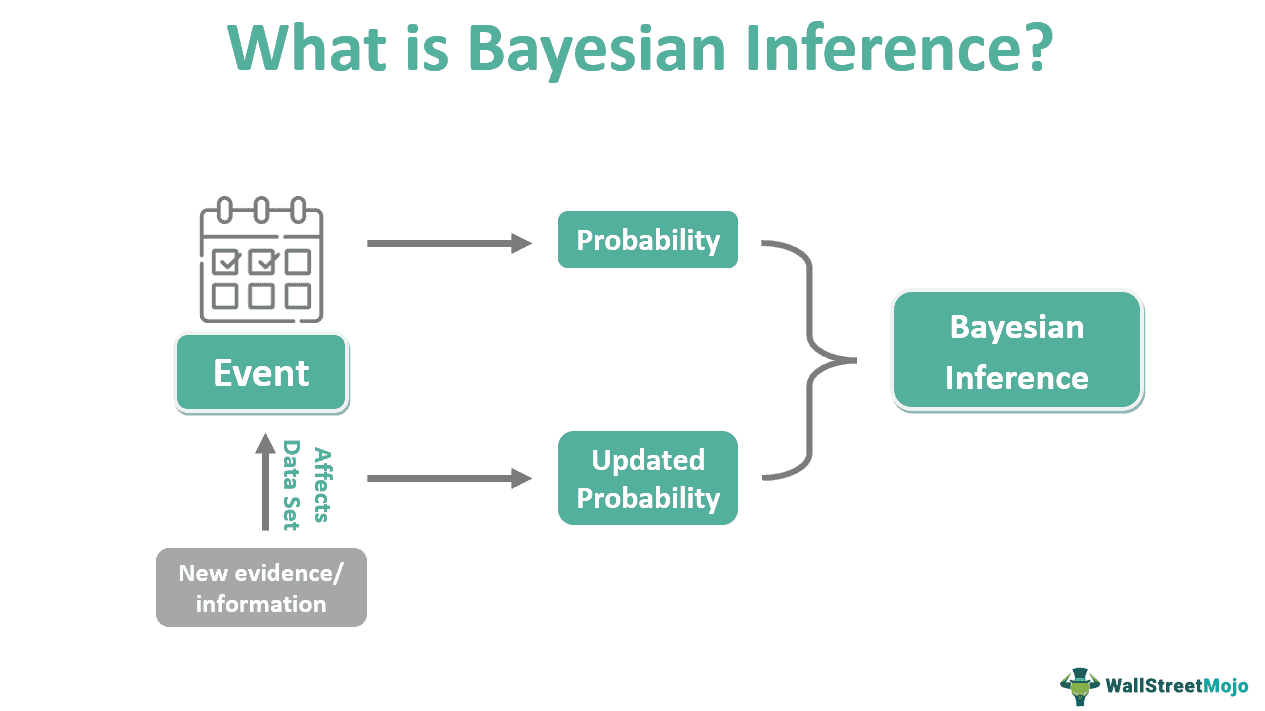
贝叶斯分析,一种统计推断方法(以英国数学家托马斯-贝叶斯命名),允许人们将关于人口参数的先验信息与样本所含信息的证据相结合,以指导统计推断过程。
statistics-lab™ 为您的留学生涯保驾护航 在代写贝叶斯分析Bayesian Analysis方面已经树立了自己的口碑, 保证靠谱, 高质且原创的统计Statistics代写服务。我们的专家在代写贝叶斯分析Bayesian Analysis代写方面经验极为丰富,各种代写贝叶斯分析Bayesian Analysis相关的作业也就用不着说。
统计代写|贝叶斯分析代写Bayesian Analysis代考|Bayesian inference
Bayesian statistical conclusions about a parameter $\theta$, or unobserved data $\tilde{y}$, are made in terms of probability statements. These probability statements are conditional on the observed value of $y$, and in our notation are written simply as $p(\theta \mid y)$ or $p(\tilde{y} \mid y)$. We also implicitly condition on the known values of any covariates, $x$. It is at the fundamental level of conditioning on observed data that Bayesian inference departs from the approach to statistical inference described in many textbooks, which is based on a retrospective evaluation of the procedure used to estimate $\theta$ (or $\tilde{y}$ ) over the distribution of possible $y$ values conditional on the true unknown value of $\theta$. Despite this difference, it will be seen that in many simple analyses, superficially similar conclusions result from the two approaches to statistical inference. However, analyses obtained using Bayesian methods can be easily extended to more complex problems. In this section, we present the basic mathematics and notation of Bayesian inference, followed in the next section by an example from genetics.
Probability notation
Some comments on notation are needed at this point. First, $p(\cdot \mid \cdot)$ denotes a conditional probability density with the arguments determined by the context, and similarly for $p(\cdot)$, which denotes a marginal distribution. We use the terms ‘distribution’ and ‘density’ interchangeably. The same notation is used for continuous density functions and discrete probability mass functions. Different distributions in the same equation (or expression) will each be denoted by $p(\cdot)$, as in (1.1) below, for example. Although an abuse of standard mathematical notation, this method is compact and similar to the standard practice of using $p(\cdot)$ for the probability of any discrete event, where the sample space is also suppressed in the notation. Depending on context, to avoid confusion, we may use the notation $\operatorname{Pr}(\cdot)$ for the probability of an event; for example, $\operatorname{Pr}(\theta>2)=\int_{\theta>2} p(\theta) d \theta$. When using a standard distribution, we use a notation based on the name of the distribution; for example, if $\theta$ has a normal distribution with mean $\mu$ and variance $\sigma^2$, we write $\theta \sim \mathrm{N}\left(\mu, \sigma^2\right)$ or $p(\theta)=\mathrm{N}\left(\theta \mid \mu, \sigma^2\right)$ or, to be even more explicit, $p\left(\theta \mid \mu, \sigma^2\right)=\mathrm{N}\left(\theta \mid \mu, \sigma^2\right)$. Throughout, we use notation such as $\mathrm{N}\left(\mu, \sigma^2\right)$ for random variables and $\mathrm{N}\left(\theta \mid \mu, \sigma^2\right)$ for density functions. Notation and formulas for several standard distributions appear in Appendix A.
We also occasionally use the following expressions for all-positive random variables $\theta$ : the coefficient of variation is defined as $\operatorname{sd}(\theta) / \mathrm{E}(\theta)$, the geometric mean is $\exp (\mathrm{E}[\log (\theta)])$, and the geometric standard deviation is $\exp (\operatorname{sd}[\log (\theta)])$.
统计代写|贝叶斯分析代写Bayesian Analysis代考|Bayes’ rule
In order to make probability statements about $\theta$ given $y$, we must begin with a model providing a joint probability distribution for $\theta$ and $y$. The joint probability mass or density function can be written as a product of two densities that are often referred to as the prior distribution $p(\theta)$ and the sampling distribution (or data distribution) $p(y \mid \theta)$, respectively:
$$
p(\theta, y)=p(\theta) p(y \mid \theta)
$$
Simply conditioning on the known value of the data $y$, using the basic property of conditional probability known as Bayes’ rule, yields the posterior density:
$$
p(\theta \mid y)=\frac{p(\theta, y)}{p(y)}=\frac{p(\theta) p(y \mid \theta)}{p(y)}
$$
where $p(y)=\sum_\theta p(\theta) p(y \mid \theta)$, and the sum is over all possible values of $\theta$ (or $p(y)=$ $\int p(\theta) p(y \mid \theta) d \theta$ in the case of continuous $\left.\theta\right)$. An equivalent form of (1.1) omits the factor $p(y)$, which does not depend on $\theta$ and, with fixed $y$, can thus be considered a constant, yielding the unnormalized posterior density, which is the right side of (1.2):
$$
p(\theta \mid y) \propto p(\theta) p(y \mid \theta)
$$
The second term in this expression, $p(y \mid \theta)$, is taken here as a function of $\theta$, not of $y$. These simple formulas encapsulate the technical core of Bayesian inference: the primary task of any specific application is to develop the model $p(\theta, y)$ and perform the computations to summarize $p(\theta \mid y)$ in appropriate ways.

贝叶斯分析代考
统计代写|贝叶斯分析代写Bayesian Analysis代考|Bayesian inference
关于参数$\theta$或未观测数据$\tilde{y}$的贝叶斯统计结论是根据概率陈述得出的。这些概率陈述以$y$的观测值为条件,在我们的符号中简单地写成$p(\theta \mid y)$或$p(\tilde{y} \mid y)$。我们还隐式地以任何协变量的已知值为条件,$x$。贝叶斯推理与许多教科书中描述的统计推断方法不同,这是在对观察到的数据进行条件反射的基本层面上,这是基于对用于估计$\theta$(或$\tilde{y}$)可能的$y$值分布的过程的回顾性评估,该分布以$\theta$的真实未知值为条件。尽管存在这种差异,但可以看到,在许多简单的分析中,两种统计推断方法得出的结论表面上相似。然而,使用贝叶斯方法得到的分析可以很容易地扩展到更复杂的问题。在本节中,我们将介绍贝叶斯推理的基本数学和符号,下一节将介绍遗传学中的一个例子。
概率符号
此时需要对符号进行一些注释。首先,$p(\cdot \mid \cdot)$表示由上下文确定参数的条件概率密度,类似地,$p(\cdot)$表示边际分布。我们交替使用“分布”和“密度”这两个术语。连续密度函数和离散概率质量函数使用相同的符号。相同方程(或表达式)中的不同分布将分别用$p(\cdot)$表示,例如,如下面的(1.1)所示。虽然滥用了标准数学符号,但这种方法很紧凑,类似于使用$p(\cdot)$表示任何离散事件的概率的标准做法,其中样本空间也在符号中被抑制。根据上下文,为了避免混淆,我们可以使用$\operatorname{Pr}(\cdot)$表示事件的概率;例如:$\operatorname{Pr}(\theta>2)=\int_{\theta>2} p(\theta) d \theta$。当使用标准分布时,我们使用基于分布名称的符号;例如,如果$\theta$有一个均值$\mu$和方差$\sigma^2$的正态分布,我们写$\theta \sim \mathrm{N}\left(\mu, \sigma^2\right)$或$p(\theta)=\mathrm{N}\left(\theta \mid \mu, \sigma^2\right)$,或者更明确地说,$p\left(\theta \mid \mu, \sigma^2\right)=\mathrm{N}\left(\theta \mid \mu, \sigma^2\right)$。在整个过程中,我们使用$\mathrm{N}\left(\mu, \sigma^2\right)$表示随机变量,$\mathrm{N}\left(\theta \mid \mu, \sigma^2\right)$表示密度函数。几个标准分布的符号和公式见附录A。
对于全正随机变量$\theta$,我们偶尔也会用到以下表达式:变异系数定义为$\operatorname{sd}(\theta) / \mathrm{E}(\theta)$,几何均值为$\exp (\mathrm{E}[\log (\theta)])$,几何标准差为$\exp (\operatorname{sd}[\log (\theta)])$。
统计代写|贝叶斯分析代写Bayesian Analysis代考|Bayes’ rule
为了对给定$y$的$\theta$做出概率陈述,我们必须从一个模型开始,该模型提供了$\theta$和$y$的联合概率分布。联合概率质量或密度函数可以写成两个密度的乘积,这两个密度通常分别称为先验分布$p(\theta)$和抽样分布(或数据分布)$p(y \mid \theta)$:
$$
p(\theta, y)=p(\theta) p(y \mid \theta)
$$
简单地对已知的数据值$y$进行调节,利用条件概率的基本属性,即贝叶斯规则,得到后验密度:
$$
p(\theta \mid y)=\frac{p(\theta, y)}{p(y)}=\frac{p(\theta) p(y \mid \theta)}{p(y)}
$$
其中$p(y)=\sum_\theta p(\theta) p(y \mid \theta)$,对$\theta$的所有可能值求和(如果连续为$\left.\theta\right)$,则为$p(y)=$$\int p(\theta) p(y \mid \theta) d \theta$)。式(1.1)的等效形式省略了不依赖于$\theta$的因子$p(y)$,当$y$固定时,可以认为是一个常数,从而得到非归一化后验密度,即式(1.2)的右侧:
$$
p(\theta \mid y) \propto p(\theta) p(y \mid \theta)
$$
这个表达式中的第二项$p(y \mid \theta)$在这里是$\theta$的函数,而不是$y$的函数。这些简单的公式概括了贝叶斯推理的技术核心:任何特定应用程序的主要任务都是开发模型$p(\theta, y)$,并以适当的方式执行计算以总结$p(\theta \mid y)$。

统计代写请认准statistics-lab™. statistics-lab™为您的留学生涯保驾护航。
金融工程代写
金融工程是使用数学技术来解决金融问题。金融工程使用计算机科学、统计学、经济学和应用数学领域的工具和知识来解决当前的金融问题,以及设计新的和创新的金融产品。
非参数统计代写
非参数统计指的是一种统计方法,其中不假设数据来自于由少数参数决定的规定模型;这种模型的例子包括正态分布模型和线性回归模型。
广义线性模型代考
广义线性模型(GLM)归属统计学领域,是一种应用灵活的线性回归模型。该模型允许因变量的偏差分布有除了正态分布之外的其它分布。
术语 广义线性模型(GLM)通常是指给定连续和/或分类预测因素的连续响应变量的常规线性回归模型。它包括多元线性回归,以及方差分析和方差分析(仅含固定效应)。
有限元方法代写
有限元方法(FEM)是一种流行的方法,用于数值解决工程和数学建模中出现的微分方程。典型的问题领域包括结构分析、传热、流体流动、质量运输和电磁势等传统领域。
有限元是一种通用的数值方法,用于解决两个或三个空间变量的偏微分方程(即一些边界值问题)。为了解决一个问题,有限元将一个大系统细分为更小、更简单的部分,称为有限元。这是通过在空间维度上的特定空间离散化来实现的,它是通过构建对象的网格来实现的:用于求解的数值域,它有有限数量的点。边界值问题的有限元方法表述最终导致一个代数方程组。该方法在域上对未知函数进行逼近。[1] 然后将模拟这些有限元的简单方程组合成一个更大的方程系统,以模拟整个问题。然后,有限元通过变化微积分使相关的误差函数最小化来逼近一个解决方案。
tatistics-lab作为专业的留学生服务机构,多年来已为美国、英国、加拿大、澳洲等留学热门地的学生提供专业的学术服务,包括但不限于Essay代写,Assignment代写,Dissertation代写,Report代写,小组作业代写,Proposal代写,Paper代写,Presentation代写,计算机作业代写,论文修改和润色,网课代做,exam代考等等。写作范围涵盖高中,本科,研究生等海外留学全阶段,辐射金融,经济学,会计学,审计学,管理学等全球99%专业科目。写作团队既有专业英语母语作者,也有海外名校硕博留学生,每位写作老师都拥有过硬的语言能力,专业的学科背景和学术写作经验。我们承诺100%原创,100%专业,100%准时,100%满意。
随机分析代写
随机微积分是数学的一个分支,对随机过程进行操作。它允许为随机过程的积分定义一个关于随机过程的一致的积分理论。这个领域是由日本数学家伊藤清在第二次世界大战期间创建并开始的。
时间序列分析代写
随机过程,是依赖于参数的一组随机变量的全体,参数通常是时间。 随机变量是随机现象的数量表现,其时间序列是一组按照时间发生先后顺序进行排列的数据点序列。通常一组时间序列的时间间隔为一恒定值(如1秒,5分钟,12小时,7天,1年),因此时间序列可以作为离散时间数据进行分析处理。研究时间序列数据的意义在于现实中,往往需要研究某个事物其随时间发展变化的规律。这就需要通过研究该事物过去发展的历史记录,以得到其自身发展的规律。
回归分析代写
多元回归分析渐进(Multiple Regression Analysis Asymptotics)属于计量经济学领域,主要是一种数学上的统计分析方法,可以分析复杂情况下各影响因素的数学关系,在自然科学、社会和经济学等多个领域内应用广泛。
MATLAB代写
MATLAB 是一种用于技术计算的高性能语言。它将计算、可视化和编程集成在一个易于使用的环境中,其中问题和解决方案以熟悉的数学符号表示。典型用途包括:数学和计算算法开发建模、仿真和原型制作数据分析、探索和可视化科学和工程图形应用程序开发,包括图形用户界面构建MATLAB 是一个交互式系统,其基本数据元素是一个不需要维度的数组。这使您可以解决许多技术计算问题,尤其是那些具有矩阵和向量公式的问题,而只需用 C 或 Fortran 等标量非交互式语言编写程序所需的时间的一小部分。MATLAB 名称代表矩阵实验室。MATLAB 最初的编写目的是提供对由 LINPACK 和 EISPACK 项目开发的矩阵软件的轻松访问,这两个项目共同代表了矩阵计算软件的最新技术。MATLAB 经过多年的发展,得到了许多用户的投入。在大学环境中,它是数学、工程和科学入门和高级课程的标准教学工具。在工业领域,MATLAB 是高效研究、开发和分析的首选工具。MATLAB 具有一系列称为工具箱的特定于应用程序的解决方案。对于大多数 MATLAB 用户来说非常重要,工具箱允许您学习和应用专业技术。工具箱是 MATLAB 函数(M 文件)的综合集合,可扩展 MATLAB 环境以解决特定类别的问题。可用工具箱的领域包括信号处理、控制系统、神经网络、模糊逻辑、小波、仿真等。