统计代写|商业分析作业代写Statistical Modelling for Business代考|Describing Central Tendency
如果你也在 怎样代写商业分析Statistical Modelling for Business这个学科遇到相关的难题,请随时右上角联系我们的24/7代写客服。
商业分析就是利用数据分析和统计的方法,来分析企业之前的商业表现,从而通过分析结果来对未来的商业战略进行预测和指导 。
statistics-lab™ 为您的留学生涯保驾护航 在代写商业分析Statistical Modelling for Business方面已经树立了自己的口碑, 保证靠谱, 高质且原创的统计Statistics代写服务。我们的专家在代写商业分析Statistical Modelling for Business方面经验极为丰富,各种代写商业分析Statistical Modelling for Business相关的作业也就用不着说。
我们提供的商业分析Statistical Modelling for Business及其相关学科的代写,服务范围广, 其中包括但不限于:
- Statistical Inference 统计推断
- Statistical Computing 统计计算
- Advanced Probability Theory 高等楖率论
- Advanced Mathematical Statistics 高等数理统计学
- (Generalized) Linear Models 广义线性模型
- Statistical Machine Learning 统计机器学习
- Longitudinal Data Analysis 纵向数据分析
- Foundations of Data Science 数据科学基础
统计代写|商业分析作业代写Statistical Modelling for Business代考|The mean, median, and mode
In addition to describing the shape of the distribution of a sample or population of measurements, we also describe the data set’s central tendency. A measure of central tendency represents the center or middle of the data. Sometimes we think of a measure of central tendency as a typical value. However, as we will see, not all measures of central tendency are necessarily typical values.
One important measure of central tendency for a population of measurements is the population mean. We define it as follows:More precisely, the population mean is calculated by adding all the population measurements and then dividing the resulting sum by the number of population measurements. For instance, suppose that Chris is a college junior majoring in business. This semester Chris is taking five classes and the numbers of students enrolled in the classes (that is, the class sizes) are as follows:
The mean $\mu$ of this population of class sizes is
$$
\mu=\frac{60+41+15+30+34}{5}=\frac{180}{5}=36
$$
Because this population of five class sizes is small, it is possible to compute the population mean. Often, however, a population is very large and we cannot obtain a measurement for each population element. Therefore, we cannot compute the population mean. In such a case, we must estimate the population mean by using a sample of measurements.
In order to understand how to estimate a population mean, we must realize that the population mean is a population parameter.
统计代写|商业分析作业代写Statistical Modelling for Business代考|The Car Mileage Case: Estimating Mileage
In order to offer its tax credit, the federal government has decided to define the “typical” EPA combined city and highway mileage for a car model as the mean $\mu$ of the population of EPA combined mileages that would be obtained by all cars of this type. Here, using the mean to represent a typical value is probably reasonable. We know that some individual cars will get mileages that are lower than the mean and some will get mileages that are above it. However, because there will be many thousands of these cars on the road, the mean mileage obtained by these cars is probably a reasonable way to represent the model’s overall fuel economy. Therefore, the government will offer its tax credit to any automaker selling a midsize model equipped with an automatic transmission that achieves a mean EPA combined mileage of at least $31 \mathrm{mpg}$.
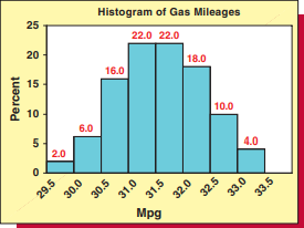
To demonstrate that its new midsize model qualifies for the tax credit, the automaker in this case study wishes to use the sample of 50 mileages in Table $3.1$ to estimate $\mu$, the model’s mean mileage. Before calculating the mean of the entire sample of 50 mileages, we will illustrate the formulas involved by calculating the mean of the first five of these mileages.
Table $3.1$ tells us that $x_{1}=30.8, x_{2}=31.7, x_{3}=30.1, x_{4}=31.6$, and $x_{5}=32.1$, so the sum of the first five mileages is
$$
\begin{aligned}
\sum_{i=1}^{5} x_{i} &=x_{1}+x_{2}+x_{3}+x_{4}+x_{5} \
&=30.8+31 . \overline{3}+30.1+31.6+3 \overline{2} .1=156.3
\end{aligned}
$$
Therefore, the mean of the first five mileages is
$$
\bar{x}=\frac{\sum_{i=1}^{5} x_{i}}{5}=\frac{156.3}{5}=31.26
$$
Of course, intuitively, we are likely to obtain a more accurate point estimate of the population mean by using all of the available sample information. The sum of all 50 mileages can be verified to be
$$
\sum_{i=1}^{50} x_{i}=x_{1}+x_{2}+\cdots+x_{50}=30.8+31.7+\cdots+31.4=1578
$$
Therefore, the mean of the sample of 50 mileages is
$$
\bar{x}=\frac{\sum_{i=1}^{50} x_{i}}{50}=\frac{1578}{50}=31.56
$$
This point estimate says we estimate that the mean mileage that would be obtained by all of the new midsize cars that will or could potentially be produced this year is $31.56 \mathrm{mpg}$. Unless we are extremely lucky, however, there will be sampling error. That is, the point estimate $\bar{x}=31.56$ mpg, which is the average of the sample of fifty randomly selected mileages, will probably not exactly equal the population mean $\mu$, which is the average mileage that would be obtained by all cars. Therefore, although $\bar{x}=31.56$ provides some evidence that $\mu$ is at least 31 and thus that the automaker should get the tax credit, it does not provide definitive evidence. In later chapters, we discuss how to assess the reliability of the sample mean and how to use a measure of reliability to decide whether sample information provides definitive evidence.
统计代写|商业分析作业代写Statistical Modelling for Business代考|Comparing the mean, median, and mode
Often we construct a histogram for a sample to make inferences about the shape of the sampled population. When we do this, it can be useful to “smooth out” the histogram and use the resulting relative frequency curve to describe the shape of the population. Relative frequency curves can have many shapes. Three common shapes are illustrated in Figure $3.3$. Part (a) of this figure depicts a population described by a symmetrical relative frequency curve. For such a population, the mean $(\mu)$, median $\left(M_{s}\right)$, and mode $\left(M_{s}\right)$ are all equal. Note that in this case all three of these quantities are located under the highest point of the curve. It follows that when the frequency distribution of a sample of measurements is approximately symmetrical, then the sample mean, median, and mode will be nearly the same. For instance,
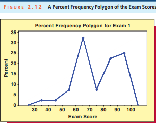
consider the sample of 50 mileages in Table 3.1. Because the histogram of these mileages in Figure $3.2$ is approximately symmetrical, the mean $-31.56$ – and the median-31.55- of the mileages are approximately equal to each other.
Figure $3.3$ (b) depicts a population that is skewed to the right. Here the population mean is larger than the population median, and the population median is larger than the population mode (the mode is located under the highest point of the relative frequency curve). In this case the population mean averages in the large values in the upper tail of the distribution. Thus the population mean is more affected by these large values than is the population median. To understand this, we consider the following example.
金融中的随机方法代写
统计代写|商业分析作业代写Statistical Modelling for Business代考|The mean, median, and mode
除了描述样本或测量群体的分布形状外,我们还描述了数据集的集中趋势。集中趋势的度量代表数据的中心或中间。有时我们将集中趋势的度量视为一个典型值。然而,正如我们将看到的,并非所有集中趋势的度量都必然是典型值。
测量群体集中趋势的一个重要度量是群体均值。我们将其定义如下:更准确地说,总体均值是通过将所有总体测量值相加,然后将所得总和除以总体测量值的数量来计算的。例如,假设 Chris 是一名商业专业的大三学生。本学期 Chris 上 5 节课,在校学生人数(即班级人数)如下:
均值μ这个班级规模的人口是
μ=60+41+15+30+345=1805=36
因为这个五个班级规模的人口很小,所以可以计算人口平均值。但是,通常人口非常大,我们无法获得每个人口元素的测量值。因此,我们无法计算总体均值。在这种情况下,我们必须使用测量样本来估计总体均值。
为了理解如何估计总体均值,我们必须认识到总体均值是总体参数。
统计代写|商业分析作业代写Statistical Modelling for Business代考|The Car Mileage Case: Estimating Mileage
为了提供税收抵免,联邦政府已决定将汽车模型的“典型”EPA 城市和高速公路组合里程定义为平均值μ这种类型的所有汽车将获得的 EPA 总里程数。在这里,用平均值来表示一个典型值可能是合理的。我们知道,有些个别汽车的行驶里程会低于平均值,而有些汽车的行驶里程会高于平均值。但是,由于道路上会有成千上万辆这样的汽车,这些汽车所获得的平均里程可能是代表该车型整体燃油经济性的合理方式。因此,政府将向任何销售配备自动变速器的中型车型的汽车制造商提供税收抵免,该车型的平均 EPA 综合里程至少为31米pG.
为了证明其新的中型车型有资格获得税收抵免,本案例研究中的汽车制造商希望使用表中 50 英里的样本3.1估计μ,模型的平均里程。在计算 50 英里的整个样本的平均值之前,我们将通过计算前 5 英里的平均值来说明所涉及的公式。
桌子3.1告诉我们X1=30.8,X2=31.7,X3=30.1,X4=31.6, 和X5=32.1,所以前五英里的总和是
∑一世=15X一世=X1+X2+X3+X4+X5 =30.8+31.3¯+30.1+31.6+32¯.1=156.3
因此,前五英里的平均值为
X¯=∑一世=15X一世5=156.35=31.26
当然,直观地说,我们很可能通过使用所有可用的样本信息来获得对总体均值的更准确的点估计。可以验证所有 50 里程的总和为
∑一世=150X一世=X1+X2+⋯+X50=30.8+31.7+⋯+31.4=1578
因此,50 英里的样本的平均值为
X¯=∑一世=150X一世50=157850=31.56
该点估计表明,我们估计今年将或可能生产的所有新中型汽车的平均行驶里程为31.56米pG. 然而,除非我们非常幸运,否则会有抽样误差。即点估计X¯=31.56mpg 是随机选择的 50 英里的样本的平均值,可能不会完全等于总体平均值μ,这是所有汽车将获得的平均里程数。因此,虽然X¯=31.56提供了一些证据表明μ至少是 31 岁,因此汽车制造商应该获得税收抵免,它没有提供确切的证据。在后面的章节中,我们将讨论如何评估样本均值的可靠性以及如何使用可靠性度量来确定样本信息是否提供了确凿的证据。
统计代写|商业分析作业代写Statistical Modelling for Business代考|Comparing the mean, median, and mode
我们经常为样本构建直方图,以推断样本总体的形状。当我们这样做时,“平滑”直方图并使用生成的相对频率曲线来描述总体形状会很有用。相对频率曲线可以有多种形状。三种常见的形状如图所示3.3. 该图的 (a) 部分描绘了由对称相对频率曲线描述的总体。对于这样的人群,均值(μ), 中位数(米s), 和模式(米s)都是平等的。请注意,在这种情况下,所有这三个量都位于曲线的最高点下方。因此,当测量样本的频率分布近似对称时,样本均值、中值和众数将几乎相同。例如,
考虑表 3.1 中 50 英里的样本。因为图中这些里程的直方图3.2近似对称,均值−31.56– 里程数的中位数 31.55- 大致相等。
数字3.3(b) 描绘了向右倾斜的人口。这里总体均值大于总体中位数,总体中位数大于总体众数(众数位于相对频率曲线最高点下方)。在这种情况下,总体平均值是分布上尾中较大值的平均值。因此,总体平均值比总体中位数更受这些大值的影响。为了理解这一点,我们考虑下面的例子。

统计代写请认准statistics-lab™. statistics-lab™为您的留学生涯保驾护航。统计代写|python代写代考
随机过程代考
在概率论概念中,随机过程是随机变量的集合。 若一随机系统的样本点是随机函数,则称此函数为样本函数,这一随机系统全部样本函数的集合是一个随机过程。 实际应用中,样本函数的一般定义在时间域或者空间域。 随机过程的实例如股票和汇率的波动、语音信号、视频信号、体温的变化,随机运动如布朗运动、随机徘徊等等。
贝叶斯方法代考
贝叶斯统计概念及数据分析表示使用概率陈述回答有关未知参数的研究问题以及统计范式。后验分布包括关于参数的先验分布,和基于观测数据提供关于参数的信息似然模型。根据选择的先验分布和似然模型,后验分布可以解析或近似,例如,马尔科夫链蒙特卡罗 (MCMC) 方法之一。贝叶斯统计概念及数据分析使用后验分布来形成模型参数的各种摘要,包括点估计,如后验平均值、中位数、百分位数和称为可信区间的区间估计。此外,所有关于模型参数的统计检验都可以表示为基于估计后验分布的概率报表。
广义线性模型代考
广义线性模型(GLM)归属统计学领域,是一种应用灵活的线性回归模型。该模型允许因变量的偏差分布有除了正态分布之外的其它分布。
statistics-lab作为专业的留学生服务机构,多年来已为美国、英国、加拿大、澳洲等留学热门地的学生提供专业的学术服务,包括但不限于Essay代写,Assignment代写,Dissertation代写,Report代写,小组作业代写,Proposal代写,Paper代写,Presentation代写,计算机作业代写,论文修改和润色,网课代做,exam代考等等。写作范围涵盖高中,本科,研究生等海外留学全阶段,辐射金融,经济学,会计学,审计学,管理学等全球99%专业科目。写作团队既有专业英语母语作者,也有海外名校硕博留学生,每位写作老师都拥有过硬的语言能力,专业的学科背景和学术写作经验。我们承诺100%原创,100%专业,100%准时,100%满意。
机器学习代写
随着AI的大潮到来,Machine Learning逐渐成为一个新的学习热点。同时与传统CS相比,Machine Learning在其他领域也有着广泛的应用,因此这门学科成为不仅折磨CS专业同学的“小恶魔”,也是折磨生物、化学、统计等其他学科留学生的“大魔王”。学习Machine learning的一大绊脚石在于使用语言众多,跨学科范围广,所以学习起来尤其困难。但是不管你在学习Machine Learning时遇到任何难题,StudyGate专业导师团队都能为你轻松解决。
多元统计分析代考
基础数据: $N$ 个样本, $P$ 个变量数的单样本,组成的横列的数据表
变量定性: 分类和顺序;变量定量:数值
数学公式的角度分为: 因变量与自变量
时间序列分析代写
随机过程,是依赖于参数的一组随机变量的全体,参数通常是时间。 随机变量是随机现象的数量表现,其时间序列是一组按照时间发生先后顺序进行排列的数据点序列。通常一组时间序列的时间间隔为一恒定值(如1秒,5分钟,12小时,7天,1年),因此时间序列可以作为离散时间数据进行分析处理。研究时间序列数据的意义在于现实中,往往需要研究某个事物其随时间发展变化的规律。这就需要通过研究该事物过去发展的历史记录,以得到其自身发展的规律。
回归分析代写
多元回归分析渐进(Multiple Regression Analysis Asymptotics)属于计量经济学领域,主要是一种数学上的统计分析方法,可以分析复杂情况下各影响因素的数学关系,在自然科学、社会和经济学等多个领域内应用广泛。
MATLAB代写
MATLAB 是一种用于技术计算的高性能语言。它将计算、可视化和编程集成在一个易于使用的环境中,其中问题和解决方案以熟悉的数学符号表示。典型用途包括:数学和计算算法开发建模、仿真和原型制作数据分析、探索和可视化科学和工程图形应用程序开发,包括图形用户界面构建MATLAB 是一个交互式系统,其基本数据元素是一个不需要维度的数组。这使您可以解决许多技术计算问题,尤其是那些具有矩阵和向量公式的问题,而只需用 C 或 Fortran 等标量非交互式语言编写程序所需的时间的一小部分。MATLAB 名称代表矩阵实验室。MATLAB 最初的编写目的是提供对由 LINPACK 和 EISPACK 项目开发的矩阵软件的轻松访问,这两个项目共同代表了矩阵计算软件的最新技术。MATLAB 经过多年的发展,得到了许多用户的投入。在大学环境中,它是数学、工程和科学入门和高级课程的标准教学工具。在工业领域,MATLAB 是高效研究、开发和分析的首选工具。MATLAB 具有一系列称为工具箱的特定于应用程序的解决方案。对于大多数 MATLAB 用户来说非常重要,工具箱允许您学习和应用专业技术。工具箱是 MATLAB 函数(M 文件)的综合集合,可扩展 MATLAB 环境以解决特定类别的问题。可用工具箱的领域包括信号处理、控制系统、神经网络、模糊逻辑、小波、仿真等。