分类: 图像处理Image Processing

CS代写|图像处理作业代写Image Processing代考|COMP345

如果你也在 怎样代写图像处理Image Processing这个学科遇到相关的难题,请随时右上角联系我们的24/7代写客服。

图像处理是使用数字计算机通过一种算法来处理数字图像。

statistics-lab™ 为您的留学生涯保驾护航 在代写图像处理Image Processing方面已经树立了自己的口碑, 保证靠谱, 高质且原创的统计Statistics代写服务。我们的专家在代写图像处理Image Processing代写方面经验极为丰富,各种代写图像处理Image Processing相关的作业也就用不着说。

我们提供的图像处理Image Processing及其相关学科的代写,服务范围广, 其中包括但不限于:

  • Statistical Inference 统计推断
  • Statistical Computing 统计计算
  • Advanced Probability Theory 高等楖率论
  • Advanced Mathematical Statistics 高等数理统计学
  • (Generalized) Linear Models 广义线性模型
  • Statistical Machine Learning 统计机器学习
  • Longitudinal Data Analysis 纵向数据分析
  • Foundations of Data Science 数据科学基础
CS代写|图像处理作业代写Image Processing代考|COMP345

CS代写|图像处理作业代写Image Processing代考|Half-Tone Output Technology

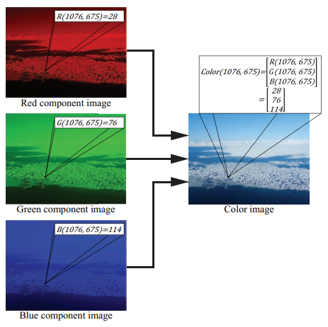
General printing equipment can only directly output binary images. For example, the grayscale output of a laser printer has only two levels (either printing, outputting black; or not printing, outputting white). To output a grayscale image on a binary image output device and maintain its original grayscale level, a technique called half-tone output is often used.
Half-tone output technology can be regarded as a technology that converts grayscale images into binary images. It converts various gray scales in the intended output image into a binary point mode so that the grayscale image can be output by a printing device that can only directly output binary points. At the same time, it takes advantage of the integrated characteristics of the human eye, by controlling the form of the output binary point pattern (including number, size, shape, etc.) to give people a visual sense of multiple gray levels. In other words, the image output by the half-tone output technology is still a binary image at a very fine scale, but due to the spatial local averaging effect of the eyes, what is perceived is a grayscale image at a coarser scale. For example, in a binary image, the gray level of each pixel is only white or black, but from a certain distance, the unit perceived by the human eye is composed of multiple pixels, then the gray level perceived by the human eye is the average gray level of all pixels in this unit (proportional to the number of black pixels).

Half-tone output technology is mainly divided into two types: amplitude modulation (AM) technology and frequency modulation (FM) technology, which will be introduced separately below.

In the beginning, the half-tone output technology proposed and used displays of different gray levels by adjusting the size of the output black dots, which can be called amplitude modulation (AM) half-tone output technology. For example, the pictures in the early newspapers used ink dots of different sizes on the grid to represent the gray scale. When viewed from a certain distance, a group of small ink dots can produce a brighter gray scale visual effect, while a group of large ink dots can produce a darker gray scale visual effect. In practice, the size of ink dots is inversely proportional to the gray scale being represented, that is, the dots printed in the bright image region are small, and the dots printed in the dark image region are larger. When the ink dot is small enough and the observation distance is long enough, the human eye can obtain a relatively continuous and smooth gray-scale image according to

the integrated characteristics. In general, the resolution of pictures in newspapers is about 100 dots per inch (DPI), while the resolution of pictures in books or magazines is about 300 DPI.

In amplitude modulation, the binary points are regularly arranged. The size of these dots varies according to the gray scale to be represented, and the shape of the dots is not a decisive factor. For example, on a laser printer, it simulates different gray scales by controlling the proportion of ink coverage, and the shape of the ink dots is not strictly controlled. When the amplitude modulation technology is used, the effect of the output binary point mode not only depends on the size of each point but also depends on the size of the grid interval. The smaller the interval, the higher the output resolution. The interval size of the grid is limited by the resolution of the printer (measured in DPI).

CS代写|图像处理作业代写Image Processing代考|Half-Tone Output Mask

A specific implementation method of half-tone output is to first subdivide the image output unit and combine the adjacent basic binary points to form the output unit so that each output unit contains several basic binary points. Let some basic binary points output black while other basic binary points output white to get different grayscale effects. In other words, to output different gray levels, a set of masks/templates needs to be established, and each mask corresponds to an output unit. Divide each mask into regular grids, and each grid corresponds to a basic binary point. By adjusting each basic binary point to black or white, each mask can output a different grayscale so as to achieve the purpose of outputting grayscale images.

If a mask is divided into $2 \times 2$ grids, five different gray levels can be output according to the way shown in Figure 1.7. If a mask is divided into $3 \times 3$ grids, ten different gray scales can be output according to the way shown in Figure 1.8. If a mask is divided into $4 \times 4$ grids, 17 different gray scales can be output according to the way shown in Figure 1.9. By analogy, if a mask is divided into $n \times n$ grids, then $n^2+1$ different gray levels can be output.
Because there are $C_k^n=n ! /(n-k) ! k !$ different methods for putting $k$ points into $n$ units, the arrangement of black points in these figures is not unique. Note that if a grid is black at a certain gray level, it will still be black in all outputs greater than that gray level.

Divide the mask into grids according to the above method, then to output 256 gray levels, a mask needs to be divided into $16 \times 16$ units, that is, $16 \times 16$ positions are used to represent one pixel. It can be seen that the spatial resolution of the output image will be greatly affected. It can be seen that the half-tone output technology is only worth using when the gray value output by the output device itself is limited, and it is a reduction in spatial resolution in exchange for an increase in amplitude resolution. Assuming that each pixel in a $2 \times 2$ matrix can be white or black, each pixel requires one bit. Regarding this $2 \times 2$ matrix as a half-tone output unit, this unit needs 4 bits and can output 5 gray scales ( 16 modes),which are $0 / 4,1 / 4,2 / 4,3 / 4$, and $4 / 4$ (or written as $0,1,2,3$, and 4). However, if a pixel is represented by four bits, the pixel can have 16 gray levels. From this point of view, when the half-tone output uses the same storage unit, if the number of output levels increases, the number of output units will decrease.

To maintain the sharpness of the details in the image, it is necessary to have more lines per inch; at the same time, to represent these details, it also needs to have more brightness levels. This requires the printer to be able to print a large number of very small dots. Dividing a template into $8 \times 8$ grids can print 65 gray scales. For printing at 125 lines per inch, this corresponds to $8 \times 125=1,000 \mathrm{dpi}$. In most applications, this is the lower limit of the printed image. Color printing requires smaller dots, and high-quality printing often requires $2,400-3,000$ dpi.

When outputting images on different media, the required resolutions are often different. For example, when an image is displayed on the screen, the number of rows per inch generally corresponds to the number of grids per inch. When displaying images in newspapers, a resolution of at least 85 lines per inch is often used; for magazines or books, a resolution of at least 133 lines or 175 lines per inch is often used.

CS代写|图像处理作业代写Image Processing代考|COMP345

图像处理代考

CS代写|图像处理作业代写Image Processing代考|Half-Tone Output Technology

一般的印刷设备只能直接输出二值图像。例如,激光打印机的灰度输出只有两个级别(打印,输出黑色;或不打印,输出白色)。为了在二进制图像输出设备上输出灰度图像并保持其原始灰度级,通常使用一种称为半色调输出的技术。
半色调输出技术可以看作是一种将灰度图像转换为二值图像的技术。它将预期输出图像中的各种灰度转换为二进制点模式,使灰度图像可以由只能直接输出二进制点的打印设备输出。同时,它利用人眼的综合特性,通过控制输出二进制点图案的形式(包括数量、大小、形状等),给人以多重灰度的视觉感受。也就是说,半色调输出技术输出的图像仍然是非常精细尺度的二值图像,但由于眼睛的空间局部平均效应,感知到的是较粗尺度的灰度图像。例如,在二值图像中,

半色调输出技术主要分为调幅(AM)技术和调频(FM)技术两种,下面分别介绍。

半色调输出技术最初是通过调整输出黑点的大小来提出和使用不同灰度的显示器,可称为调幅(AM)半色调输出技术。例如,早期报纸上的图片在网格上使用不同大小的墨点来表示灰度。从一定距离看,一组小墨点可以产生较亮的灰度视觉效果,而一组大墨点可以产生较暗的灰度视觉效果。在实际应用中,墨点的大小与所代表的灰度成反比,即在亮图像区域打印的墨点较小,在暗图像区域打印的墨点较大。当墨点足够小,观察距离足够长时,

综合特征。一般来说,报纸上图片的分辨率约为每英寸100点(DPI),而书籍或杂志上的图片分辨率约为300 DPI。

在幅度调制中,二进制点是规则排列的。这些点的大小根据要表示的灰度而变化,点的形状不是决定性因素。比如在激光打印机上,通过控制墨水覆盖的比例来模拟不同的灰度,对墨点的形状没有严格控制。使用幅度调制技术时,输出二进制点模式的效果不仅取决于每个点的大小,还取决于网格间隔的大小。间隔越小,输出分辨率越高。网格的间隔大小受打印机分辨率的限制(以 DPI 为单位)。

CS代写|图像处理作业代写Image Processing代考|Half-Tone Output Mask

半色调输出的一种具体实现方法是先对图像输出单元进行细分,将相邻的基本二进制点组合形成输出单元,使得每个输出单元包含若干个基本二进制点。让一些基本二进制点输出黑色,而其他基本二进制点输出白色,以获得不同的灰度效果。也就是说,要输出不同的灰度级,需要建立一组掩码/模板,每个掩码对应一个输出单元。将每个掩码分成规则的网格,每个网格对应一个基本的二进制点。通过将每个基本二进制点调整为黑色或白色,每个掩模可以输出不同的灰度,从而达到输出灰度图像的目的。

如果一个掩码分为2×2格,按照图 1.7 所示的方式可以输出五种不同的灰度。如果一个掩码分为3×3格,按照图 1.8 所示的方式可以输出十种不同的灰度。如果一个掩码分为4×4格,按照图 1.9 所示的方式可以输出 17 种不同的灰度。以此类推,如果一个面具被分为n×n格子,然后n2+1可以输出不同的灰度。
因为有Cķn=n!/(n−ķ)!ķ!不同的放置方法ķ指向n单位,这些图中黑点的排列并不是唯一的。请注意,如果网格在某个灰度级为黑色,则在所有大于该灰度级的输出中仍将是黑色。

按照上面的方法将mask划分成网格,那么要输出256个灰度级,需要将一个mask划分为16×16单位,即16×16位置用于表示一个像素。可以看出,输出图像的空间分辨率会受到很大影响。可见,半色调输出技术只有在输出设备本身输出的灰度值有限的情况下才值得使用,它是以空间分辨率的降低换取幅度分辨率的提高。假设每个像素在2×2矩阵可以是白色或黑色,每个像素需要一位。关于这个2×2矩阵作为半色调输出单元,该单元需要 4 位,可以输出 5 种灰度(16 种模式),分别是0/4,1/4,2/4,3/4, 和4/4(或写成0,1,2,3, 和 4)。但是,如果一个像素用 4 位表示,则该像素可以有 16 个灰度级。由此看来,当半色调输出使用相同的存储单元时,如果输出级数增加,输出单元数会减少。

为了保持图像中细节的清晰度,每英寸必须有更多的线条;同时,为了表现这些细节,还需要有更多的亮度等级。这就要求打印机能够打印大量非常小的点。将模板划分为8×8网格可以打印65个灰度。对于以每英寸 125 行打印,这对应于8×125=1,000dp一世. 在大多数应用中,这是打印图像的下限。彩色打印需要更小的网点,而高质量打印通常需要2,400−3,000dpi。

在不同媒体上输出图像时,所需的分辨率往往不同。例如,在屏幕上显示图像时,每英寸的行数通常对应于每英寸的网格数。在报纸上显示图像时,通常使用至少 85 行/英寸的分辨率;对于杂志或书籍,通常使用每英寸至少 133 行或 175 行的分辨率。

CS代写|图像处理作业代写Image Processing代考 请认准statistics-lab™

统计代写请认准statistics-lab™. statistics-lab™为您的留学生涯保驾护航。

金融工程代写

金融工程是使用数学技术来解决金融问题。金融工程使用计算机科学、统计学、经济学和应用数学领域的工具和知识来解决当前的金融问题,以及设计新的和创新的金融产品。

非参数统计代写

非参数统计指的是一种统计方法,其中不假设数据来自于由少数参数决定的规定模型;这种模型的例子包括正态分布模型和线性回归模型。

广义线性模型代考

广义线性模型(GLM)归属统计学领域,是一种应用灵活的线性回归模型。该模型允许因变量的偏差分布有除了正态分布之外的其它分布。

术语 广义线性模型(GLM)通常是指给定连续和/或分类预测因素的连续响应变量的常规线性回归模型。它包括多元线性回归,以及方差分析和方差分析(仅含固定效应)。

有限元方法代写

有限元方法(FEM)是一种流行的方法,用于数值解决工程和数学建模中出现的微分方程。典型的问题领域包括结构分析、传热、流体流动、质量运输和电磁势等传统领域。

有限元是一种通用的数值方法,用于解决两个或三个空间变量的偏微分方程(即一些边界值问题)。为了解决一个问题,有限元将一个大系统细分为更小、更简单的部分,称为有限元。这是通过在空间维度上的特定空间离散化来实现的,它是通过构建对象的网格来实现的:用于求解的数值域,它有有限数量的点。边界值问题的有限元方法表述最终导致一个代数方程组。该方法在域上对未知函数进行逼近。[1] 然后将模拟这些有限元的简单方程组合成一个更大的方程系统,以模拟整个问题。然后,有限元通过变化微积分使相关的误差函数最小化来逼近一个解决方案。

tatistics-lab作为专业的留学生服务机构,多年来已为美国、英国、加拿大、澳洲等留学热门地的学生提供专业的学术服务,包括但不限于Essay代写,Assignment代写,Dissertation代写,Report代写,小组作业代写,Proposal代写,Paper代写,Presentation代写,计算机作业代写,论文修改和润色,网课代做,exam代考等等。写作范围涵盖高中,本科,研究生等海外留学全阶段,辐射金融,经济学,会计学,审计学,管理学等全球99%专业科目。写作团队既有专业英语母语作者,也有海外名校硕博留学生,每位写作老师都拥有过硬的语言能力,专业的学科背景和学术写作经验。我们承诺100%原创,100%专业,100%准时,100%满意。

随机分析代写


随机微积分是数学的一个分支,对随机过程进行操作。它允许为随机过程的积分定义一个关于随机过程的一致的积分理论。这个领域是由日本数学家伊藤清在第二次世界大战期间创建并开始的。

时间序列分析代写

随机过程,是依赖于参数的一组随机变量的全体,参数通常是时间。 随机变量是随机现象的数量表现,其时间序列是一组按照时间发生先后顺序进行排列的数据点序列。通常一组时间序列的时间间隔为一恒定值(如1秒,5分钟,12小时,7天,1年),因此时间序列可以作为离散时间数据进行分析处理。研究时间序列数据的意义在于现实中,往往需要研究某个事物其随时间发展变化的规律。这就需要通过研究该事物过去发展的历史记录,以得到其自身发展的规律。

回归分析代写

多元回归分析渐进(Multiple Regression Analysis Asymptotics)属于计量经济学领域,主要是一种数学上的统计分析方法,可以分析复杂情况下各影响因素的数学关系,在自然科学、社会和经济学等多个领域内应用广泛。

MATLAB代写

MATLAB 是一种用于技术计算的高性能语言。它将计算、可视化和编程集成在一个易于使用的环境中,其中问题和解决方案以熟悉的数学符号表示。典型用途包括:数学和计算算法开发建模、仿真和原型制作数据分析、探索和可视化科学和工程图形应用程序开发,包括图形用户界面构建MATLAB 是一个交互式系统,其基本数据元素是一个不需要维度的数组。这使您可以解决许多技术计算问题,尤其是那些具有矩阵和向量公式的问题,而只需用 C 或 Fortran 等标量非交互式语言编写程序所需的时间的一小部分。MATLAB 名称代表矩阵实验室。MATLAB 最初的编写目的是提供对由 LINPACK 和 EISPACK 项目开发的矩阵软件的轻松访问,这两个项目共同代表了矩阵计算软件的最新技术。MATLAB 经过多年的发展,得到了许多用户的投入。在大学环境中,它是数学、工程和科学入门和高级课程的标准教学工具。在工业领域,MATLAB 是高效研究、开发和分析的首选工具。MATLAB 具有一系列称为工具箱的特定于应用程序的解决方案。对于大多数 MATLAB 用户来说非常重要,工具箱允许您学习应用专业技术。工具箱是 MATLAB 函数(M 文件)的综合集合,可扩展 MATLAB 环境以解决特定类别的问题。可用工具箱的领域包括信号处理、控制系统、神经网络、模糊逻辑、小波、仿真等。

R语言代写问卷设计与分析代写
PYTHON代写回归分析与线性模型代写
MATLAB代写方差分析与试验设计代写
STATA代写机器学习/统计学习代写
SPSS代写计量经济学代写
EVIEWS代写时间序列分析代写
EXCEL代写深度学习代写
SQL代写各种数据建模与可视化代写

CS代写|图像处理作业代写Image Processing代考|ELE454

如果你也在 怎样代写图像处理Image Processing这个学科遇到相关的难题,请随时右上角联系我们的24/7代写客服。

图像处理是使用数字计算机通过一种算法来处理数字图像。

statistics-lab™ 为您的留学生涯保驾护航 在代写图像处理Image Processing方面已经树立了自己的口碑, 保证靠谱, 高质且原创的统计Statistics代写服务。我们的专家在代写图像处理Image Processing代写方面经验极为丰富,各种代写图像处理Image Processing相关的作业也就用不着说。

我们提供的图像处理Image Processing及其相关学科的代写,服务范围广, 其中包括但不限于:

  • Statistical Inference 统计推断
  • Statistical Computing 统计计算
  • Advanced Probability Theory 高等楖率论
  • Advanced Mathematical Statistics 高等数理统计学
  • (Generalized) Linear Models 广义线性模型
  • Statistical Machine Learning 统计机器学习
  • Longitudinal Data Analysis 纵向数据分析
  • Foundations of Data Science 数据科学基础
CS代写|图像处理作业代写Image Processing代考|ELE454

CS代写|图像处理作业代写Image Processing代考|Images and Pixels

The objective world is three-dimensional (3-D) in space, but the image obtained from the objective scene is generally two-dimensional (2-D). An image can be represented by a 2-D array $f(x, y)$, where $x$ and $y$ represent the position of a coordinate point in the 2-D space $X Y$, and $f$ represents the image value of a property $F$ at a certain point $(x, y)$. For example, $f$ in a grayscale image represents a gray value, which often corresponds to the observed brightness of an objective scene. Text images are often binary images, and there are only two values for $f$, corresponding to text and blank space, respectively. The image at the point $(x, y)$ can also have multiple properties at the same time. In this case, it can be represented by a vector $f$. For example, a color image has three values of red, green, and blue at each image point, which can be recorded as $\left[f_r(x, y), f_g(x, y), f_b(x, y)\right]$. It needs to be pointed out that people always use images according to the different properties at different positions in the image.

An image can represent the spatial distribution of radiant energy. This distribution can be a function of five variables $T(x, y, z, t, \lambda)$, where $x, y$, and $z$ are spatial variables,

and $t$ represents time variables, $\lambda$ is wavelength (corresponding to the spectral variable). For example, a red object reflects light with a wavelength of $0.57-0.78 \mu \mathrm{m}$ and absorbs almost all energy of other wavelengths; a green object reflects light with a wavelength of $0.48-0.57 \mu \mathrm{m}$; a blue object reflects light with a wavelength of $0.40-0.48 \mu \mathrm{m}$. Ultraviolet (color) objects reflect light with a wavelength of $0.25-0.40 \mu \mathrm{m}$, and infrared (color) objects reflect light with a wavelength of $0.78-1.5 \mu \mathrm{m}$. Together, they cover a wavelength range of $0.25-1.5 \mu \mathrm{m}$. Since the actual image is finite in time and space, $T(x, y, z, t, \lambda)$ is a 5-D finite function.

The images acquired in the early years are mostly continuous (analog), that is, the values of $f, x$, and $y$ can be any real numbers. With the invention of the computer and the development of electronic equipment, the acquired images are all discrete (digital) and can be processed directly by the computer. Someone once used $I(r, c)$ to represent a digital image, where the values of $I, r$, and $c$ are all integers. Here $I$ represents the discretized $f ;(r, c)$ represents the discretized $(x, y)$, where $r$ represents the image row, and $c$ represents the image column. The discussion in this book is related to digital images. Images or $f(x, y)$ are used to represent digital images without causing confusion. Unless otherwise specified, $f, x$, and $y$ are all taken their values in the integer set.

In the early days, the term “picture” was generally used to refer to images. With the development of digital technology, the term “image” is now used to represent a discretized “image” because “computers store numerical images of a picture or scene” (Zhang 1996). Each basic unit in an image is called an image element, and in the early days, when the “picture” was used to represent an image, it was called a pixel. For 2-D images, “pel” has also been used to refer to the basic unit. If one collects a series of 2-D images or uses some special equipment, one can also get 3-D images. For 3-D images, voxel is often used to represent the basic unit. Someone has also suggested to use “imel” to represent various image units.

CS代写|图像处理作业代写Image Processing代考|Spatial Resolution and Amplitude Resolution

From the above introduction and discussion of image representation and display, it can be known that the content of a 2-D grayscale image is determined by the number of pixels (the number of rows of the image multiplied by the number of columns of the image) and by the number of gray levels for each pixel. The former determines the spatial resolution of the image, while the latter determines the amplitude resolution of the image. From the perspective of image acquisition, the acquisition of images is to record the spatial distribution of the light reflection intensity of the scene within a certain field of view. The accuracy in the spatial field of view here corresponds to the spatial resolution of the image, and the accuracy in the intensity range corresponds to the amplitude resolution of the image. The former corresponds to the number of digitized spatial sampling points while the latter corresponds to the quantization levels of the sampling point value (for grayscale images, it refers to gray levels; for depth images, it refers to depth levels). They are all important performance indicators of image acquisition devices.

The spatial resolution and amplitude resolution of the image are determined by sampling and quantization, respectively. Taking a typical CCD camera as an example, the spatial resolution of the image is mainly determined by the size and arrangement of the photoelectric sensing units in the image acquisition matrix in the camera, and the amplitude resolution of the grayscale image is mainly determined by the number of stages in the quantization of the electrical signal intensity. As shown in Figure 1.3, the signal radiated from the photoreceptive unit in the image acquisition matrix is sampled in space and quantized in intensity.

The sampling process can be seen as dividing the image plane into regular grids. The position of each grid is determined by a pair of Cartesian coordinates $(x, y)$, where $x$ and $y$ are integers. Let $f(\cdot)$ be a function that assigns gray values to the grid point $(x, y)$, where $f$ is an integer in $F$, then $f(x, y)$ is a digital image, and this assignment process is a quantization process.

From the perspective of computer processing of images, an image must be discretized in space and gray level before it can be processed by the computer. The discretization of spatial coordinates is called spatial sampling (abbreviated as sampling), which determines the spatial resolution of the image; the discretization of gray values is called grayscale quantization (abbreviated as quantization), which determines the amplitude resolution of the image.

CS代写|图像处理作业代写Image Processing代考|ELE454

图像处理代考

CS代写|图像处理作业代写Image Processing代考|Images and Pixels

客观世界在空间上是三维的(3-D),但从客观场景得到的图像一般是二维的(2-D)。图像可以用二维数组表示F(X,是), 在哪里X和是表示坐标点在二维空间中的位置X是, 和F表示属性的图像值F在某一点(X,是). 例如,F在灰度图像中表示一个灰度值,它通常对应于观察到的客观场景的亮度。文本图像通常是二值图像,只有两个值F,分别对应文本和空格。该点的图像(X,是)也可以同时拥有多个属性。在这种情况下,它可以用一个向量来表示F. 例如,一幅彩色图像在每个图像点上具有红、绿、蓝三个值,可以记为[Fr(X,是),FG(X,是),Fb(X,是)]. 需要指出的是,人们总是根据图像中不同位置的不同属性来使用图像。

图像可以表示辐射能量的空间分布。该分布可以是五个变量的函数吨(X,是,和,吨,l), 在哪里X,是, 和和是空间变量,

和吨表示时间变量,l是波长(对应于光谱变量)。例如,红色物体反射波长为0.57−0.78米米并吸收几乎所有其他波长的能量;绿色物体反射波长为0.48−0.57米米; 蓝色物体反射波长为0.40−0.48米米. 紫外线(彩色)物体反射波长为0.25−0.40米米, 红外(彩色)物体反射波长为0.78−1.5米米. 它们共同覆盖的波长范围为0.25−1.5米米. 由于实际图像在时间和空间上是有限的,吨(X,是,和,吨,l)是一个 5-D 有限函数。

早年获取的图像大多是连续的(模拟的),即F,X, 和是可以是任何实数。随着计算机的发明和电子设备的发展,所获取的图像都是离散的(数字的),可以直接由计算机处理。曾经有人用过我(r,C)表示数字图像,其中的值我,r, 和C都是整数。这里我表示离散的F;(r,C)表示离散的(X,是), 在哪里r表示图像行,并且C表示图像列。本书中的讨论与数字图像有关。图像或F(X,是)用于表示数字图像而不会引起混淆。除非另有规定,F,X, 和是都在整数集中取它们的值。

在早期,“图片”一词通常用于指代图像。随着数字技术的发展,“图像”一词现在被用来表示离散化的“图像”,因为“计算机存储了图片或场景的数字图像”(Zhang 1996)。图像中的每个基本单元称为图像元素,在早期,当“图片”用于表示图像时,称为像素。对于二维图像,“pel”也被用来指代基本单位。如果收集一系列 2-D 图像或使用一些特殊设备,也可以得到 3-D 图像。对于 3D 图像,通常使用体素来表示基本单位。也有人建议使用“imel”来表示各种图像单元。

CS代写|图像处理作业代写Image Processing代考|Spatial Resolution and Amplitude Resolution

从以上对图像表示和显示的介绍和讨论可知,一张二维灰度图像的内容是由像素数(图像的行数乘以图像的列数)决定的) 和每个像素的灰度级数。前者决定了图像的空间分辨率,而后者决定了图像的幅度分辨率。从图像采集的角度来看,图像的采集就是记录一定视野内场景的光反射强度的空间分布。这里的空间视场精度对应于图像的空间分辨率,强度范围内的精度对应于图像的幅度分辨率。前者对应的是数字化的空间采样点的个数,后者对应的是采样点值的量化级别(对于灰度图像,它是指灰度级;对于深度图像,它是指深度级别)。它们都是图像采集设备的重要性能指标。

图像的空间分辨率和幅度分辨率分别由采样和量化决定。以典型的CCD相机为例,图像的空间分辨率主要由相机内图像采集矩阵中光电传感单元的大小和排列方式决定,而灰度图像的幅值分辨率主要由电信号强度量化的阶段数。如图 1.3 所示,从图像采集矩阵中的感光单元辐射的信号在空间中进行采样并在强度上进行量化。

采样过程可以看作是将图像平面划分为规则的网格。每个网格的位置由一对笛卡尔坐标确定(X,是), 在哪里X和是是整数。让F(⋅)是一个将灰度值分配给网格点的函数(X,是), 在哪里F是一个整数F, 然后F(X,是)是数字图像,这个赋值过程是一个量化过程。

从计算机处理图像的角度来看,图像必须在空间和灰度上进行离散化,才能被计算机处理。空间坐标的离散化称为空间采样(简称采样),它决定了图像的空间分辨率;灰度值的离散化称为灰度量化(简称量化),它决定了图像的幅值分辨率。

CS代写|图像处理作业代写Image Processing代考 请认准statistics-lab™

统计代写请认准statistics-lab™. statistics-lab™为您的留学生涯保驾护航。

金融工程代写

金融工程是使用数学技术来解决金融问题。金融工程使用计算机科学、统计学、经济学和应用数学领域的工具和知识来解决当前的金融问题,以及设计新的和创新的金融产品。

非参数统计代写

非参数统计指的是一种统计方法,其中不假设数据来自于由少数参数决定的规定模型;这种模型的例子包括正态分布模型和线性回归模型。

广义线性模型代考

广义线性模型(GLM)归属统计学领域,是一种应用灵活的线性回归模型。该模型允许因变量的偏差分布有除了正态分布之外的其它分布。

术语 广义线性模型(GLM)通常是指给定连续和/或分类预测因素的连续响应变量的常规线性回归模型。它包括多元线性回归,以及方差分析和方差分析(仅含固定效应)。

有限元方法代写

有限元方法(FEM)是一种流行的方法,用于数值解决工程和数学建模中出现的微分方程。典型的问题领域包括结构分析、传热、流体流动、质量运输和电磁势等传统领域。

有限元是一种通用的数值方法,用于解决两个或三个空间变量的偏微分方程(即一些边界值问题)。为了解决一个问题,有限元将一个大系统细分为更小、更简单的部分,称为有限元。这是通过在空间维度上的特定空间离散化来实现的,它是通过构建对象的网格来实现的:用于求解的数值域,它有有限数量的点。边界值问题的有限元方法表述最终导致一个代数方程组。该方法在域上对未知函数进行逼近。[1] 然后将模拟这些有限元的简单方程组合成一个更大的方程系统,以模拟整个问题。然后,有限元通过变化微积分使相关的误差函数最小化来逼近一个解决方案。

tatistics-lab作为专业的留学生服务机构,多年来已为美国、英国、加拿大、澳洲等留学热门地的学生提供专业的学术服务,包括但不限于Essay代写,Assignment代写,Dissertation代写,Report代写,小组作业代写,Proposal代写,Paper代写,Presentation代写,计算机作业代写,论文修改和润色,网课代做,exam代考等等。写作范围涵盖高中,本科,研究生等海外留学全阶段,辐射金融,经济学,会计学,审计学,管理学等全球99%专业科目。写作团队既有专业英语母语作者,也有海外名校硕博留学生,每位写作老师都拥有过硬的语言能力,专业的学科背景和学术写作经验。我们承诺100%原创,100%专业,100%准时,100%满意。

随机分析代写


随机微积分是数学的一个分支,对随机过程进行操作。它允许为随机过程的积分定义一个关于随机过程的一致的积分理论。这个领域是由日本数学家伊藤清在第二次世界大战期间创建并开始的。

时间序列分析代写

随机过程,是依赖于参数的一组随机变量的全体,参数通常是时间。 随机变量是随机现象的数量表现,其时间序列是一组按照时间发生先后顺序进行排列的数据点序列。通常一组时间序列的时间间隔为一恒定值(如1秒,5分钟,12小时,7天,1年),因此时间序列可以作为离散时间数据进行分析处理。研究时间序列数据的意义在于现实中,往往需要研究某个事物其随时间发展变化的规律。这就需要通过研究该事物过去发展的历史记录,以得到其自身发展的规律。

回归分析代写

多元回归分析渐进(Multiple Regression Analysis Asymptotics)属于计量经济学领域,主要是一种数学上的统计分析方法,可以分析复杂情况下各影响因素的数学关系,在自然科学、社会和经济学等多个领域内应用广泛。

MATLAB代写

MATLAB 是一种用于技术计算的高性能语言。它将计算、可视化和编程集成在一个易于使用的环境中,其中问题和解决方案以熟悉的数学符号表示。典型用途包括:数学和计算算法开发建模、仿真和原型制作数据分析、探索和可视化科学和工程图形应用程序开发,包括图形用户界面构建MATLAB 是一个交互式系统,其基本数据元素是一个不需要维度的数组。这使您可以解决许多技术计算问题,尤其是那些具有矩阵和向量公式的问题,而只需用 C 或 Fortran 等标量非交互式语言编写程序所需的时间的一小部分。MATLAB 名称代表矩阵实验室。MATLAB 最初的编写目的是提供对由 LINPACK 和 EISPACK 项目开发的矩阵软件的轻松访问,这两个项目共同代表了矩阵计算软件的最新技术。MATLAB 经过多年的发展,得到了许多用户的投入。在大学环境中,它是数学、工程和科学入门和高级课程的标准教学工具。在工业领域,MATLAB 是高效研究、开发和分析的首选工具。MATLAB 具有一系列称为工具箱的特定于应用程序的解决方案。对于大多数 MATLAB 用户来说非常重要,工具箱允许您学习应用专业技术。工具箱是 MATLAB 函数(M 文件)的综合集合,可扩展 MATLAB 环境以解决特定类别的问题。可用工具箱的领域包括信号处理、控制系统、神经网络、模糊逻辑、小波、仿真等。

R语言代写问卷设计与分析代写
PYTHON代写回归分析与线性模型代写
MATLAB代写方差分析与试验设计代写
STATA代写机器学习/统计学习代写
SPSS代写计量经济学代写
EVIEWS代写时间序列分析代写
EXCEL代写深度学习代写
SQL代写各种数据建模与可视化代写

机器视觉代写|图像处理作业代写Image Processing代考|Ice Edge Detection

如果你也在 怎样代写图像处理Image Processing这个学科遇到相关的难题,请随时右上角联系我们的24/7代写客服。

图像处理是使用数字计算机通过一种算法来处理数字图像。

statistics-lab™ 为您的留学生涯保驾护航 在代写图像处理Image Processing方面已经树立了自己的口碑, 保证靠谱, 高质且原创的统计Statistics代写服务。我们的专家在代写图像处理Image Processing代写方面经验极为丰富,各种代写图像处理Image Processing相关的作业也就用不着说。

我们提供的图像处理Image Processing及其相关学科的代写,服务范围广, 其中包括但不限于:

  • Statistical Inference 统计推断
  • Statistical Computing 统计计算
  • Advanced Probability Theory 高等楖率论
  • Advanced Mathematical Statistics 高等数理统计学
  • (Generalized) Linear Models 广义线性模型
  • Statistical Machine Learning 统计机器学习
  • Longitudinal Data Analysis 纵向数据分析
  • Foundations of Data Science 数据科学基础
机器视觉代写|图像处理作业代写Image Processing代考|Ice Edge Detection

机器视觉代写|图像处理作业代写Image Processing代考|GRADIENT OPERATOR

The gradient, which is the first-order derivative, has a direction toward the most rapid change in intensity. The gradient of a digital image with pixel value $f(x, y)$ is defined as the vector:
$$
\nabla f=\left[\begin{array}{l}
G_{x} \
G_{y}
\end{array}\right]=\left[\begin{array}{l}
\frac{\partial f}{\partial x} \
\frac{\partial f}{\partial y}
\end{array}\right]
$$
and the gradient magnitude is given by:
$$
|\nabla f|=\sqrt{G_{x}^{2}+G_{y}^{2}}=\sqrt{\left(\frac{\partial f}{\partial x}\right)^{2}+\left(\frac{\partial f}{\partial y}\right)^{2}}
$$

while the direction of the gradient vector is given by the angle:
$$
\theta=\angle f=\arctan \left(\frac{G_{x}}{G_{y}}\right)
$$
with respect to the $x$-axis, where for implementation we use the arctan() function for correct quadrant mapping.

For computational efficiency, the gradient magnitude is sometimes approximated by using the squared gradient magnitude:
$$
\nabla f \approx G_{x}^{2}+G_{y}^{2}
$$
or the absolute gradient magnitude:
$$
\nabla f \approx\left|G_{x}\right|+\left|G_{y}\right|
$$
where these two approximations also preserve the relative changes in intensity scales.
The gradient of an image can be used for the detection of edges in the image; it requires the calculation of the partial derivatives $G_{x}$ and $G_{y}$ at every pixel location in the image. To directly estimate the partial derivatives $G_{x}$ and $G_{y}$ is one of the key issues in this method. The discrete approximation of partial derivatives over a neighborhood about a point is required. For example, it is a common and simple way to form the running difference of pixels along rows and columns of the image, which gives the approximation:
$$
\begin{aligned}
&\frac{\partial f}{\partial x}(x, y) \approx f(x+1, y)-f(x, y) \
&\frac{\partial f}{\partial y}(x, y) \approx f(x, y+1)-f(x, y)
\end{aligned}
$$
To implement the derivatives over an entire image, the edge detector, which is a local image processing method designed to detect edge pixels, filters the image with convolution kernels. So, the Equations $4.6 \mathrm{a}$ and $4.6 \mathrm{~b}$ can then be implemented for all pertinent values of $x$ and $y$ by filtering $f(x, y)$ with the simple 1-dimensional convolution kernels shown in Figure 4.1.

机器视觉代写|图像处理作业代写Image Processing代考|LAPLACIAN

Similar to the first-order derivative, the second-order derivative, which is the Laplacian of the image, is defined as:
$$
\nabla^{2} f=\frac{\partial^{2} f}{\partial x^{2}}+\frac{\partial^{2} f}{\partial y^{2}}
$$
The second-order derivative along the $x$ direction can be approximated by differentiating Equation $4.6 \mathrm{a}$ with respect to $x$, e.g.:
$$
\begin{aligned}
\frac{\partial^{2} f}{\partial x^{2}}(x, y) & \approx \frac{\partial G_{x}(x, y)}{\partial x} \
&=\frac{\partial f(x+1, y)}{\partial x}-\frac{\partial f(x, y)}{\partial x} \
& \approx[f(x+2, y)-f(x+1, y)]-[f(x+1, y)-f(x, y)] \
&=f(x+2, y)-2 f(x+1, y)+f(x, y)
\end{aligned}
$$

Since this approximation is centered about the pixel $(x+1, y)$, however, we replace $x$ with $x-1$ and obtain the result:
$$
\frac{\partial^{2} f}{\partial x^{2}}(x, y) \approx f(x+1, y)+f(x-1, y)-2 f(x, y)
$$
This is the desired approximation to the second partial derivative centered about the pixel $(x, y)$. Similarly,
$$
\frac{\partial^{2} f}{\partial y^{2}}(x, y) \approx f(x, y+1)+f(x, y-1)-2 f(x, y)
$$
Combining Equations $4.11$ and $4.12$ two equations into a single operator according to Equation $4.9$ gives an approximation of the Laplacian:
$$
\nabla^{2} f(x, y)=f(x-1, y)+f(x+1, y)+f(x, y-1)+f(x, y+1)-4 f(x, y)
$$
This expression simply measures the weighted differences between a pixel and its 4-neighbors, and it can be implemented by using the kernel in Figure 4.4(a).

Sometimes it is desired to give more weight to the center pixels in the neighborhood, and Equation $4.13$ can be extended to include the diagonal terms, for instance, using the kernel in Figure 4.4(b).

机器视觉代写|图像处理作业代写Image Processing代考|MORPHOLOGICAL EDGE DETECTION

Morphology refers to geometrical characteristics related to the form and structure of objects, such as size, shape, and orientation. In image processing, mathematical morphology involves geometric analysis of shapes and textures in images based on some simple mathematical concepts from set theory. It is used to extract image components that are useful in representation and description of region shapes, such as boundaries, skeletons, convex hull, etc.

Morphological operators work with an image and a structuring element. The structuring element is a small set or subimage used to probe the given image for specific properties. It is also known as a kernel, and can be represented as a matrix of 0 s and Is. Values of 1 in the matrix indicate the points that belong to the structuring element, while values of 0 indicate otherwise. The structuring element has a desired shape, such as square, rectangle, disk, diamond, etc. The origin of a structuring element identifies the pixel of interest (the pixel being processed), and it must be clearly specified. The origin is typically at the center of gravity; however, it could be located at any desired position of the structuring element. Figure $4.7$ shows examples of different structuring elements of various sizes with their origins highlighted in the corresponding geometric centers.

机器视觉代写|图像处理作业代写Image Processing代考|Ice Edge Detection

图像处理代考

机器视觉代写|图像处理作业代写Image Processing代考|GRADIENT OPERATOR

梯度是一阶导数,具有强度变化最快的方向。具有像素值的数字图像的梯度F(X,是)定义为向量:
∇F=[GX G是]=[∂F∂X ∂F∂是]
梯度幅度由下式给出:
|∇F|=GX2+G是2=(∂F∂X)2+(∂F∂是)2

而梯度向量的方向由角度给出:
θ=∠F=反正切⁡(GXG是)
相对于该X-axis,为了实现,我们使用 arctan() 函数进行正确的象限映射。

为了计算效率,梯度幅度有时通过使用平方梯度幅度来近似:
∇F≈GX2+G是2
或绝对梯度幅度:
∇F≈|GX|+|G是|
其中这两个近似值还保留了强度尺度的相对变化。
图像的梯度可以用于图像边缘的检测;它需要计算偏导数GX和G是在图像中的每个像素位置。直接估计偏导数GX和G是是该方法的关键问题之一。需要对一个点的邻域进行偏导数的离散逼近。例如,形成图像沿行和列的像素运行差异是一种常见且简单的方法,它给出了近似值:
∂F∂X(X,是)≈F(X+1,是)−F(X,是) ∂F∂是(X,是)≈F(X,是+1)−F(X,是)
为了在整个图像上实现导数,边缘检测器是一种旨在检测边缘像素的局部图像处理方法,它使用卷积核对图像进行过滤。所以,方程4.6一种和4.6 b然后可以为所有相关值实现X和是通过过滤F(X,是)使用图 4.1 所示的简单一维卷积核。

机器视觉代写|图像处理作业代写Image Processing代考|LAPLACIAN

与一阶导数类似,二阶导数,即图像的拉普拉斯算子,定义为:
∇2F=∂2F∂X2+∂2F∂是2
沿的二阶导数X方向可以通过微分方程来近似4.6一种关于X,例如:
∂2F∂X2(X,是)≈∂GX(X,是)∂X =∂F(X+1,是)∂X−∂F(X,是)∂X ≈[F(X+2,是)−F(X+1,是)]−[F(X+1,是)−F(X,是)] =F(X+2,是)−2F(X+1,是)+F(X,是)

由于该近似值以像素为中心(X+1,是),但是,我们替换X和X−1并获得结果:
∂2F∂X2(X,是)≈F(X+1,是)+F(X−1,是)−2F(X,是)
这是以像素为中心的二阶偏导数的所需近似值(X,是). 相似地,
∂2F∂是2(X,是)≈F(X,是+1)+F(X,是−1)−2F(X,是)
组合方程4.11和4.12根据方程式将两个方程式合并为一个运算符4.9给出拉普拉斯算子的近似值:
∇2F(X,是)=F(X−1,是)+F(X+1,是)+F(X,是−1)+F(X,是+1)−4F(X,是)
这个表达式只是测量一个像素与其 4 个相邻像素之间的加权差异,它可以通过使用图 4.4(a) 中的内核来实现。

有时需要给邻域中的中心像素更多的权重,并且等式4.13可以扩展到包括对角项,例如,使用图 4.4(b) 中的内核。

机器视觉代写|图像处理作业代写Image Processing代考|MORPHOLOGICAL EDGE DETECTION

形态学是指与物体的形式和结构有关的几何特征,如大小、形状和方向。在图像处理中,数学形态学涉及基于集合论中的一些简单数学概念对图像中的形状和纹理进行几何分析。它用于提取对区域形状的表示和描述有用的图像分量,例如边界、骨架、凸包等。

形态学运算符使用图像和结构元素。结构元素是一个小的集合或子图像,用于探测给定图像的特定属性。也称为核,可以表示为 0 s 和 Is 的矩阵。矩阵中的值为 1 表示属于结构元素的点,而值为 0 表示其他情况。结构化元素具有所需的形状,例如正方形、矩形、圆盘、菱形等。结构化元素的原点标识感兴趣的像素(正在处理的像素),并且必须明确指定。原点通常位于重心;但是,它可以位于结构元素的任何所需位置。数字4.7显示了各种尺寸的不同结构元素的示例,它们的起源在相应的几何中心突出显示。

机器视觉代写|图像处理作业代写Image Processing代考 请认准statistics-lab™

统计代写请认准statistics-lab™. statistics-lab™为您的留学生涯保驾护航。

金融工程代写

金融工程是使用数学技术来解决金融问题。金融工程使用计算机科学、统计学、经济学和应用数学领域的工具和知识来解决当前的金融问题,以及设计新的和创新的金融产品。

非参数统计代写

非参数统计指的是一种统计方法,其中不假设数据来自于由少数参数决定的规定模型;这种模型的例子包括正态分布模型和线性回归模型。

广义线性模型代考

广义线性模型(GLM)归属统计学领域,是一种应用灵活的线性回归模型。该模型允许因变量的偏差分布有除了正态分布之外的其它分布。

术语 广义线性模型(GLM)通常是指给定连续和/或分类预测因素的连续响应变量的常规线性回归模型。它包括多元线性回归,以及方差分析和方差分析(仅含固定效应)。

有限元方法代写

有限元方法(FEM)是一种流行的方法,用于数值解决工程和数学建模中出现的微分方程。典型的问题领域包括结构分析、传热、流体流动、质量运输和电磁势等传统领域。

有限元是一种通用的数值方法,用于解决两个或三个空间变量的偏微分方程(即一些边界值问题)。为了解决一个问题,有限元将一个大系统细分为更小、更简单的部分,称为有限元。这是通过在空间维度上的特定空间离散化来实现的,它是通过构建对象的网格来实现的:用于求解的数值域,它有有限数量的点。边界值问题的有限元方法表述最终导致一个代数方程组。该方法在域上对未知函数进行逼近。[1] 然后将模拟这些有限元的简单方程组合成一个更大的方程系统,以模拟整个问题。然后,有限元通过变化微积分使相关的误差函数最小化来逼近一个解决方案。

tatistics-lab作为专业的留学生服务机构,多年来已为美国、英国、加拿大、澳洲等留学热门地的学生提供专业的学术服务,包括但不限于Essay代写,Assignment代写,Dissertation代写,Report代写,小组作业代写,Proposal代写,Paper代写,Presentation代写,计算机作业代写,论文修改和润色,网课代做,exam代考等等。写作范围涵盖高中,本科,研究生等海外留学全阶段,辐射金融,经济学,会计学,审计学,管理学等全球99%专业科目。写作团队既有专业英语母语作者,也有海外名校硕博留学生,每位写作老师都拥有过硬的语言能力,专业的学科背景和学术写作经验。我们承诺100%原创,100%专业,100%准时,100%满意。

随机分析代写


随机微积分是数学的一个分支,对随机过程进行操作。它允许为随机过程的积分定义一个关于随机过程的一致的积分理论。这个领域是由日本数学家伊藤清在第二次世界大战期间创建并开始的。

时间序列分析代写

随机过程,是依赖于参数的一组随机变量的全体,参数通常是时间。 随机变量是随机现象的数量表现,其时间序列是一组按照时间发生先后顺序进行排列的数据点序列。通常一组时间序列的时间间隔为一恒定值(如1秒,5分钟,12小时,7天,1年),因此时间序列可以作为离散时间数据进行分析处理。研究时间序列数据的意义在于现实中,往往需要研究某个事物其随时间发展变化的规律。这就需要通过研究该事物过去发展的历史记录,以得到其自身发展的规律。

回归分析代写

多元回归分析渐进(Multiple Regression Analysis Asymptotics)属于计量经济学领域,主要是一种数学上的统计分析方法,可以分析复杂情况下各影响因素的数学关系,在自然科学、社会和经济学等多个领域内应用广泛。

MATLAB代写

MATLAB 是一种用于技术计算的高性能语言。它将计算、可视化和编程集成在一个易于使用的环境中,其中问题和解决方案以熟悉的数学符号表示。典型用途包括:数学和计算算法开发建模、仿真和原型制作数据分析、探索和可视化科学和工程图形应用程序开发,包括图形用户界面构建MATLAB 是一个交互式系统,其基本数据元素是一个不需要维度的数组。这使您可以解决许多技术计算问题,尤其是那些具有矩阵和向量公式的问题,而只需用 C 或 Fortran 等标量非交互式语言编写程序所需的时间的一小部分。MATLAB 名称代表矩阵实验室。MATLAB 最初的编写目的是提供对由 LINPACK 和 EISPACK 项目开发的矩阵软件的轻松访问,这两个项目共同代表了矩阵计算软件的最新技术。MATLAB 经过多年的发展,得到了许多用户的投入。在大学环境中,它是数学、工程和科学入门和高级课程的标准教学工具。在工业领域,MATLAB 是高效研究、开发和分析的首选工具。MATLAB 具有一系列称为工具箱的特定于应用程序的解决方案。对于大多数 MATLAB 用户来说非常重要,工具箱允许您学习应用专业技术。工具箱是 MATLAB 函数(M 文件)的综合集合,可扩展 MATLAB 环境以解决特定类别的问题。可用工具箱的领域包括信号处理、控制系统、神经网络、模糊逻辑、小波、仿真等。

R语言代写问卷设计与分析代写
PYTHON代写回归分析与线性模型代写
MATLAB代写方差分析与试验设计代写
STATA代写机器学习/统计学习代写
SPSS代写计量经济学代写
EVIEWS代写时间序列分析代写
EXCEL代写深度学习代写
SQL代写各种数据建模与可视化代写

机器视觉代写|图像处理作业代写Image Processing代考|Ice Pixel Detection

如果你也在 怎样代写图像处理Image Processing这个学科遇到相关的难题,请随时右上角联系我们的24/7代写客服。

图像处理是使用数字计算机通过一种算法来处理数字图像。

statistics-lab™ 为您的留学生涯保驾护航 在代写图像处理Image Processing方面已经树立了自己的口碑, 保证靠谱, 高质且原创的统计Statistics代写服务。我们的专家在代写图像处理Image Processing代写方面经验极为丰富,各种代写图像处理Image Processing相关的作业也就用不着说。

我们提供的图像处理Image Processing及其相关学科的代写,服务范围广, 其中包括但不限于:

  • Statistical Inference 统计推断
  • Statistical Computing 统计计算
  • Advanced Probability Theory 高等楖率论
  • Advanced Mathematical Statistics 高等数理统计学
  • (Generalized) Linear Models 广义线性模型
  • Statistical Machine Learning 统计机器学习
  • Longitudinal Data Analysis 纵向数据分析
  • Foundations of Data Science 数据科学基础
机器视觉代写|图像处理作业代写Image Processing代考|Ice Pixel Detection

机器视觉代写|图像处理作业代写Image Processing代考|THRESHOLDING

The pixels in the same region have similar intensity. Based on that ice is whiter than water, the pixel values are normally very different between ice and water pixels, and thresholding is thus a natural choice to segment ice regions from water regions.
The thresholding method is based on the pixel’s grayscale value. It extracts the objects from the background and converts the grayscale image into a binary image. Assuming that an object is brighter than the background, the object and background pixels have intensity levels grouped into two dominant modes. The threshold $T$ is selected to distinguish the objects from the background. A pixel is marked as “object” if its value is greater than the threshold value and as “background” otherwise, that is:
$$
g(x, y)= \begin{cases}1 & \text { if } f(x, y)>T \ 0 & \text { if } f(x, y) \leq T\end{cases}
$$
where $g(x, y)$ and $f(x, y)$ are the pixel intensity values located in the $x^{\text {th }}$ row, $y^{\text {th }}$ column of the binary and grayscale image, respectively. This turns the grayscale image into a binary image.

When a constant threshold value is used over the entire image, it is called global thresholding. Otherwise, it is called variable thresholding, which allows the threshold to vary across the image.

机器视觉代写|图像处理作业代写Image Processing代考|GLOBAL THRESHOLDING

When the intensity distributions of objects and background pixels in an image are sufficiently distinct, it is possible to use a global threshold applicable for the entire image. The key to using the global thresholding is in how to select the threshold value, for which there are several different methods.

As mentioned in Section 2.2, image histogram is a useful tool for thresholding. If a histogram has a deep and sharp valley (local minima) between two peaks (local maxima), e.g., the bimodal histogram as shown in Figure 3.1, that represent objects and background, respectively, an appropriate value for the threshold will be in the valley between the two peaks in the histogram.

For example, as seen in Figure 3.2, the histogram of the grayscale sea ice image in Figure 3.2(a) clearly has two distinct modes, one for the objects (sea ice) and the other for the background (water). A suitable threshold for separating these two modes can be chosen at the bottom of this valley. As a result, it is easy to choose a threshold $T=125$ that separates them. Then the grayscale image can be converted into the binary image as shown in Figure $3.2(\mathrm{c})$, and the ice concentration is thereby estimated as $41.47 \%$.

This method is very simple. However, it is often difficult to detect the valley bottom precisely, especially when the image histogram is “noisy”, causing many local minima and maxima. Often the objects and background modes in the histogram are not distinct, making it more difficult to determine where the background intensities end and the object intensities begin. Furthermore, in most applications there are usually enough variability between images such that, even if a global thresholding is feasible, an algorithm capable of automatically estimating the threshold value for each image will be most accurate.

机器视觉代写|图像处理作业代写Image Processing代考|Otsu thresholding

To automatically select an optimal value for the threshold, Otsu proposed a method from the viewpoint of discriminant analysis; it directly approaches the feasibility of evaluating the “goodness” of the threshold [114].

Let $[0,1,2, \cdots, L-1]$ denote the $L$ intensity levels for a given image with size $M \times N$, and let $n_{i}$ denote the number of pixels with intensity $i$. The total number of pixels in the image, denoted by $n$, is then:
$$
n=M \times N=\sum_{i=0}^{L-1} n_{i}
$$
To examine the formulation of this method, the histogram is normalized as a discrete probability density function:
$$
p_{i}=\frac{n_{i}}{n}, \quad p_{i} \geq 0, \sum_{i=0}^{L-1} p_{i}=1
$$
Now suppose that a threshold $t(0<t<L-1)$ is chosen to divide the pixels into two classes $C_{0}$ and $C_{1}$, where $C_{0}$ is the set of pixels with levels $[0,1, \cdots, t]$, and $C_{1}$ is the set of pixels with levels $[t+1, t+2, \cdots, L-1]$. Then the probabilities of class $C_{0}$ occurrence is given by the cumulative sum:
$$
P_{0}(t)=P\left(C_{0}\right)=\sum_{i=0}^{l} p_{i}
$$
Similarly, the probability of class $C_{1}$ occurrence is given by
$$
P_{1}(t)=P\left(C_{1}\right)=\sum_{i=l+1}^{L-1} p_{i}=1-P_{0}(t)
$$
The mean intensity of the pixels in class $C_{0}$ is given by:
$$
\begin{aligned}
m_{0}(t) &=\sum_{i=0}^{t} i P\left(i \mid C_{0}\right) \
&=\sum_{i=0}^{t} i \frac{P\left(C_{0} \mid i\right) P(i)}{P\left(C_{0}\right)} \
&=\frac{1}{P_{0}(t)} \sum_{i=0}^{t} i p_{i}
\end{aligned}
$$
where $P\left(C_{0} \mid i\right)=1, P(i)=p_{i}$, and $P\left(C_{0}\right)=P_{0}(t)$. Similarly, the mean intensity of the pixels in class $C_{1}$ is given by:
$$
\begin{aligned}
m_{1}(t) &=\sum_{i=l+1}^{L-1} i P\left(i \mid C_{0}\right) \
&=\frac{1}{P_{1}(t)} \sum_{i=l+1}^{L-1} i p_{i}
\end{aligned}
$$

机器视觉代写|图像处理作业代写Image Processing代考|Ice Pixel Detection

图像处理代考

机器视觉代写|图像处理作业代写Image Processing代考|THRESHOLDING

同一区域中的像素具有相似的强度。基于冰比水更白,冰和水像素之间的像素值通常非常不同,因此阈值化是从水区域分割冰区域的自然选择。
阈值方法是基于像素的灰度值。它从背景中提取对象并将灰度图像转换为二值图像。假设一个物体比背景亮,物体和背景像素的强度等级分为两种主要模式。门槛吨被选中以将对象与背景区分开来。如果像素值大于阈值,则将其标记为“对象”,否则将其标记为“背景”,即:
G(X,是)={1 如果 F(X,是)>吨 0 如果 F(X,是)≤吨
在哪里G(X,是)和F(X,是)是位于Xth 排,是th 二值和灰度图像的列,分别。这会将灰度图像变成二值图像。

当在整个图像上使用恒定阈值时,称为全局阈值。否则,它被称为可变阈值,它允许阈值在图像中变化。

机器视觉代写|图像处理作业代写Image Processing代考|GLOBAL THRESHOLDING

当图像中物体和背景像素的强度分布足够明显时,可以使用适用于整个图像的全局阈值。使用全局阈值的关键是如何选择阈值,有几种不同的方法。

如 2.2 节所述,图像直方图是一个有用的阈值工具。如果直方图在两个峰(局部最大值)之间有一个深而尖的谷(局部最小值),例如,如图 3.1 所示的双峰直方图,分别代表对象和背景,则阈值的适当值将在直方图中两个峰值之间的谷值。

例如,如图 3.2 所示,图 3.2(a) 中灰度海冰图像的直方图显然具有两种不同的模式,一种用于物体(海冰),另一种用于背景(水)。可以在该谷底选择用于分离这两种模式的合适阈值。结果,很容易选择一个阈值吨=125将它们分开。然后可以将灰度图像转换为二值图像,如图3.2(C),因此冰浓度估计为41.47%.

这个方法很简单。然而,准确检测谷底往往很困难,尤其是当图像直方图“有噪声”时,会导致许多局部最小值和最大值。通常,直方图中的对象和背景模式并不明显,因此更难以确定背景强度的结束位置和对象强度的开始位置。此外,在大多数应用中,图像之间通常存在足够的可变性,因此即使全局阈值是可行的,能够自动估计每个图像的阈值的算法也将是最准确的。

机器视觉代写|图像处理作业代写Image Processing代考|Otsu thresholding

为了自动选择阈值的最佳值,Otsu 从判别分析的角度提出了一种方法;它直接接近评估阈值“好坏”的可行性[114]。

让[0,1,2,⋯,大号−1]表示大号具有大小的给定图像的强度级别米×ñ, 然后让n一世表示具有强度的像素数一世. 图像中的像素总数,表示为n, 那么:
n=米×ñ=∑一世=0大号−1n一世
为了检查该方法的公式,将直方图归一化为离散概率密度函数:
p一世=n一世n,p一世≥0,∑一世=0大号−1p一世=1
现在假设一个阈值吨(0<吨<大号−1)选择将像素分为两类C0和C1, 在哪里C0是具有级别的像素集[0,1,⋯,吨], 和C1是具有级别的像素集[吨+1,吨+2,⋯,大号−1]. 然后是类的概率C0发生由累积和给出:
磷0(吨)=磷(C0)=∑一世=0lp一世
同样,类的概率C1发生由
磷1(吨)=磷(C1)=∑一世=l+1大号−1p一世=1−磷0(吨)
类中像素的平均强度C0是(谁)给的:
米0(吨)=∑一世=0吨一世磷(一世∣C0) =∑一世=0吨一世磷(C0∣一世)磷(一世)磷(C0) =1磷0(吨)∑一世=0吨一世p一世
在哪里磷(C0∣一世)=1,磷(一世)=p一世, 和磷(C0)=磷0(吨). 同样,类中像素的平均强度C1是(谁)给的:
米1(吨)=∑一世=l+1大号−1一世磷(一世∣C0) =1磷1(吨)∑一世=l+1大号−1一世p一世

机器视觉代写|图像处理作业代写Image Processing代考 请认准statistics-lab™

统计代写请认准statistics-lab™. statistics-lab™为您的留学生涯保驾护航。

金融工程代写

金融工程是使用数学技术来解决金融问题。金融工程使用计算机科学、统计学、经济学和应用数学领域的工具和知识来解决当前的金融问题,以及设计新的和创新的金融产品。

非参数统计代写

非参数统计指的是一种统计方法,其中不假设数据来自于由少数参数决定的规定模型;这种模型的例子包括正态分布模型和线性回归模型。

广义线性模型代考

广义线性模型(GLM)归属统计学领域,是一种应用灵活的线性回归模型。该模型允许因变量的偏差分布有除了正态分布之外的其它分布。

术语 广义线性模型(GLM)通常是指给定连续和/或分类预测因素的连续响应变量的常规线性回归模型。它包括多元线性回归,以及方差分析和方差分析(仅含固定效应)。

有限元方法代写

有限元方法(FEM)是一种流行的方法,用于数值解决工程和数学建模中出现的微分方程。典型的问题领域包括结构分析、传热、流体流动、质量运输和电磁势等传统领域。

有限元是一种通用的数值方法,用于解决两个或三个空间变量的偏微分方程(即一些边界值问题)。为了解决一个问题,有限元将一个大系统细分为更小、更简单的部分,称为有限元。这是通过在空间维度上的特定空间离散化来实现的,它是通过构建对象的网格来实现的:用于求解的数值域,它有有限数量的点。边界值问题的有限元方法表述最终导致一个代数方程组。该方法在域上对未知函数进行逼近。[1] 然后将模拟这些有限元的简单方程组合成一个更大的方程系统,以模拟整个问题。然后,有限元通过变化微积分使相关的误差函数最小化来逼近一个解决方案。

tatistics-lab作为专业的留学生服务机构,多年来已为美国、英国、加拿大、澳洲等留学热门地的学生提供专业的学术服务,包括但不限于Essay代写,Assignment代写,Dissertation代写,Report代写,小组作业代写,Proposal代写,Paper代写,Presentation代写,计算机作业代写,论文修改和润色,网课代做,exam代考等等。写作范围涵盖高中,本科,研究生等海外留学全阶段,辐射金融,经济学,会计学,审计学,管理学等全球99%专业科目。写作团队既有专业英语母语作者,也有海外名校硕博留学生,每位写作老师都拥有过硬的语言能力,专业的学科背景和学术写作经验。我们承诺100%原创,100%专业,100%准时,100%满意。

随机分析代写


随机微积分是数学的一个分支,对随机过程进行操作。它允许为随机过程的积分定义一个关于随机过程的一致的积分理论。这个领域是由日本数学家伊藤清在第二次世界大战期间创建并开始的。

时间序列分析代写

随机过程,是依赖于参数的一组随机变量的全体,参数通常是时间。 随机变量是随机现象的数量表现,其时间序列是一组按照时间发生先后顺序进行排列的数据点序列。通常一组时间序列的时间间隔为一恒定值(如1秒,5分钟,12小时,7天,1年),因此时间序列可以作为离散时间数据进行分析处理。研究时间序列数据的意义在于现实中,往往需要研究某个事物其随时间发展变化的规律。这就需要通过研究该事物过去发展的历史记录,以得到其自身发展的规律。

回归分析代写

多元回归分析渐进(Multiple Regression Analysis Asymptotics)属于计量经济学领域,主要是一种数学上的统计分析方法,可以分析复杂情况下各影响因素的数学关系,在自然科学、社会和经济学等多个领域内应用广泛。

MATLAB代写

MATLAB 是一种用于技术计算的高性能语言。它将计算、可视化和编程集成在一个易于使用的环境中,其中问题和解决方案以熟悉的数学符号表示。典型用途包括:数学和计算算法开发建模、仿真和原型制作数据分析、探索和可视化科学和工程图形应用程序开发,包括图形用户界面构建MATLAB 是一个交互式系统,其基本数据元素是一个不需要维度的数组。这使您可以解决许多技术计算问题,尤其是那些具有矩阵和向量公式的问题,而只需用 C 或 Fortran 等标量非交互式语言编写程序所需的时间的一小部分。MATLAB 名称代表矩阵实验室。MATLAB 最初的编写目的是提供对由 LINPACK 和 EISPACK 项目开发的矩阵软件的轻松访问,这两个项目共同代表了矩阵计算软件的最新技术。MATLAB 经过多年的发展,得到了许多用户的投入。在大学环境中,它是数学、工程和科学入门和高级课程的标准教学工具。在工业领域,MATLAB 是高效研究、开发和分析的首选工具。MATLAB 具有一系列称为工具箱的特定于应用程序的解决方案。对于大多数 MATLAB 用户来说非常重要,工具箱允许您学习应用专业技术。工具箱是 MATLAB 函数(M 文件)的综合集合,可扩展 MATLAB 环境以解决特定类别的问题。可用工具箱的领域包括信号处理、控制系统、神经网络、模糊逻辑、小波、仿真等。

R语言代写问卷设计与分析代写
PYTHON代写回归分析与线性模型代写
MATLAB代写方差分析与试验设计代写
STATA代写机器学习/统计学习代写
SPSS代写计量经济学代写
EVIEWS代写时间序列分析代写
EXCEL代写深度学习代写
SQL代写各种数据建模与可视化代写

机器视觉代写|图像处理作业代写Image Processing代考|BILINEAR INTERPOLATION

如果你也在 怎样代写图像处理Image Processing这个学科遇到相关的难题,请随时右上角联系我们的24/7代写客服。

图像处理是使用数字计算机通过一种算法来处理数字图像。

statistics-lab™ 为您的留学生涯保驾护航 在代写图像处理Image Processing方面已经树立了自己的口碑, 保证靠谱, 高质且原创的统计Statistics代写服务。我们的专家在代写图像处理Image Processing代写方面经验极为丰富,各种代写图像处理Image Processing相关的作业也就用不着说。

我们提供的图像处理Image Processing及其相关学科的代写,服务范围广, 其中包括但不限于:

  • Statistical Inference 统计推断
  • Statistical Computing 统计计算
  • Advanced Probability Theory 高等楖率论
  • Advanced Mathematical Statistics 高等数理统计学
  • (Generalized) Linear Models 广义线性模型
  • Statistical Machine Learning 统计机器学习
  • Longitudinal Data Analysis 纵向数据分析
  • Foundations of Data Science 数据科学基础
机器视觉代写|图像处理作业代写Image Processing代考|BILINEAR INTERPOLATION

机器视觉代写|图像处理作业代写Image Processing代考|BILINEAR INTERPOLATION

The bilinear interpolation, also called first-order interpolation, calculates the intensity value for any point $(u, v)$ in the input image by using a low-degree polynomial of the form:
$$
f(u, v)=\sum_{m=0}^{1} \sum_{n=0}^{1} a_{m n} u^{m} v^{n}
$$
where the function $f$ gives the intensity value at $(u, v), a_{m n}(m, n=0,1)$ are coefficients determined by the four nearest neighbors.

When the intensity values of the four nearest neighbors are known, the general idea of the bilinear interpolation is to use linear interpolations along the $x$ – and $y$ directions to determine the intensity value at $(u, v)$. As exemplified in Figure $2.24, P$ denotes the interpolated point for which an intensity value must be calculated, $(u, v)$

are its coordinates mapped from the output image by Equation $2.33$, and $P_{1}, P_{2}, P_{3}$, and $P_{4}$ are its four nearest neighbors in the input image with the coordinates $(i, j)$, $(i, j+1),(i+1, j)$, and $(i+1, j+1)$, respectively. The bilinear interpolation first interpolates linearly along the $x$-direction to find the values at $Q_{1}$ and $Q_{2}$ :
$$
\begin{aligned}
&f\left(Q_{1}\right)=(j+1-v) f\left(P_{1}\right)+(v-j) f\left(P_{2}\right) \
&f\left(Q_{2}\right)=(j+1-v) f\left(P_{3}\right)+(v-j) f\left(P_{4}\right)
\end{aligned}
$$
then interpolates linearly along $y$-direction to obtain the value of $P$ :
$$
\begin{aligned}
f(P)=&(i+1-u) f\left(Q_{1}\right)+(u-i) f\left(Q_{2}\right) \
=&(i+1-u)\left[(j+1-v) f\left(P_{1}\right)+(v-j) f\left(P_{2}\right)\right] \
&+(u-i)\left[(j+1-v) f\left(P_{3}\right)+(v-j) f\left(P_{4}\right)\right] \
=&(i+1-u)(j+1-v) f\left(P_{1}\right)+(i+1-u)(v-j) f\left(P_{2}\right) \
&+(u-i)(j+1-v) f\left(P_{3}\right)+(u-i)(v-j) f\left(P_{4}\right)
\end{aligned}
$$
which gives:
$$
f(P)=[i+1-u \quad u-i]\left[\begin{array}{cc}
f\left(P_{1}\right) & f\left(P_{2}\right) \
f\left(P_{3}\right) & f\left(P_{4}\right)
\end{array}\right]\left[\begin{array}{c}
j+1-v \
v-j
\end{array}\right]
$$

机器视觉代写|图像处理作业代写Image Processing代考|BICUBIC INTERPOLATION

The bicubic interpolation, also called third-order interpolation, calculates the intensity value of any point $(u, v)$ in the input image by reconstructing a surface among its four nearest neighbors based on their intensity values, the derivatives in both $x$ – and $y$-directions, and the cross derivatives.

Similar to the bilinear interpolation, the bicubic interpolation calculates the intensity value for a point $(u, v)$ by fitting a cubic polynomial:
$$
f(u, v)=\sum_{m=0}^{3} \sum_{n=0}^{3} a_{m n} u^{m} v^{n}
$$
where $a_{m n}(m, n=0,1,2,3)$ are coefficients determined by its $4 \times 4$ nearest neighbors in the input image, that is, the four nearest neighbors of the point $(u, v)$ (empty circles as seen in Figure 2.25), and their horizontal, vertical, and diagonal neighboring pixels (black dots as seen in Figure 2.25). The latter are used to calculate the first-order derivatives in both $x$ – and $y$-directions and the cross derivative at each of the four nearest neighbors of point $(u, v)$. Then 8 first-order derivatives in both the $x$ – and $y$ directions and 4 cross derivatives, together with 4 intensity values at the four nearest neighbors of point $(u, v)$ give a linear system of 16 equations to determine the 16 coefficients of $a_{m n}$ in Equation $2.39$ [122].

机器视觉代写|图像处理作业代写Image Processing代考|Bicubic interpolation

Instead of directly calculating the solution of this linear system, typically by some matrix inversion, an alternative approach is to use a cubic convolution interpolation kernel that is composed of piecewise cubic polynomials defined on the subintervals $(-2,-1),(-1,0),(0,1)$, and $(1,2)[78]$. Assume the coordinates of the four nearest neighbors of point $(u, v)$ in the input image are $(i, j),(i, j+1),(i+1, j)$, and $(i+$ $1, j+1)$. Then the interpolated pixel intensity may be expressed in the compact form [121]:
$$
f(u, v)=\sum_{m=-1}^{2} \sum_{n=-1}^{2} f(u+m, v+n) r_{c}{(m+i-u)} r_{c}{-(n+j-v)}
$$
36
Sea Ice Image Processing with MATLAB
where $r_{c}(x)$ denotes a bicubic interpolation function, given by :
$$
r_{c}(x)= \begin{cases}(a+2)|x|^{3}-(a+3)|x|^{2}+1, & \text { if } 0 \leq|x| \leq 1 \ a|x|^{3}-5 a|x|^{2}+8 a|x|-4 a, & \text { if } 1<|x| \leq 2 \ 0, & \text { if }|x|>2\end{cases}
$$
where $a$ is the weighting factor that can be used as a tuning parameter to obtain a best visual interpolation result [118].

Compared with the bilinear interpolation, the bicubic interpolation method extends the influence of more neighboring pixels, and it takes not only the intensity values but also the intensity derivatives into account. Therefore, this method can produce more clear result than the bilinear interpolation method; however, at the expense of more computational complexity.

机器视觉代写|图像处理作业代写Image Processing代考|BILINEAR INTERPOLATION

图像处理代考

机器视觉代写|图像处理作业代写Image Processing代考|BILINEAR INTERPOLATION

双线性插值,也称为一阶插值,计算任意点的强度值(在,在)在输入图像中使用以下形式的低次多项式:
F(在,在)=∑米=01∑n=01一种米n在米在n
函数在哪里F给出强度值(在,在),一种米n(米,n=0,1)是由四个最近邻确定的系数。

当四个最近邻的强度值已知时,双线性插值的一般思想是沿X- 和是确定强度值的方向(在,在). 如图所示2.24,磷表示必须计算强度值的插值点,(在,在)

是通过公式从输出图像映射的坐标2.33, 和磷1,磷2,磷3, 和磷4是它在输入图像中的四个最近邻,坐标(一世,j), (一世,j+1),(一世+1,j), 和(一世+1,j+1), 分别。双线性插值首先沿线性插值X- 找到值的方向问1和问2 :
F(问1)=(j+1−在)F(磷1)+(在−j)F(磷2) F(问2)=(j+1−在)F(磷3)+(在−j)F(磷4)
然后沿线性插值是- 获取值的方向磷:
F(磷)=(一世+1−在)F(问1)+(在−一世)F(问2) =(一世+1−在)[(j+1−在)F(磷1)+(在−j)F(磷2)] +(在−一世)[(j+1−在)F(磷3)+(在−j)F(磷4)] =(一世+1−在)(j+1−在)F(磷1)+(一世+1−在)(在−j)F(磷2) +(在−一世)(j+1−在)F(磷3)+(在−一世)(在−j)F(磷4)
这使:
F(磷)=[一世+1−在在−一世][F(磷1)F(磷2) F(磷3)F(磷4)][j+1−在 在−j]

机器视觉代写|图像处理作业代写Image Processing代考|BICUBIC INTERPOLATION

双三次插值,也称为三阶插值,计算任意点的强度值(在,在)在输入图像中,通过基于其强度值在其四个最近邻居之间重建一个表面,两者中的导数X- 和是-方向和交叉导数。

与双线性插值类似,双三次插值计算一个点的强度值(在,在)通过拟合三次多项式:
F(在,在)=∑米=03∑n=03一种米n在米在n
在哪里一种米n(米,n=0,1,2,3)是由其确定的系数4×4输入图像中的最近邻,即该点的四个最近邻(在,在)(如图 2.25 所示的空圆圈),以及它们的水平、垂直和对角相邻像素(如图 2.25 所示的黑点)。后者用于计算两者的一阶导数X- 和是- 点的四个最近邻居中的每一个的方向和交叉导数(在,在). 然后 8 个一阶导数X- 和是方向和 4 个交叉导数,以及点的四个最近邻居的 4 个强度值(在,在)给出一个由 16 个方程组成的线性系统来确定 16 个系数一种米n在方程2.39 [122].

机器视觉代写|图像处理作业代写Image Processing代考|Bicubic interpolation

代替直接计算这个线性系统的解,通常通过一些矩阵求逆,另一种方法是使用三次卷积插值内核,该内核由定义在子区间上的分段三次多项式组成(−2,−1),(−1,0),(0,1), 和(1,2)[78]. 假设点的四个最近邻的坐标(在,在)在输入图像中是(一世,j),(一世,j+1),(一世+1,j), 和(一世+ 1,j+1). 然后插值像素强度可以用紧凑的形式表示[121]:
F(在,在)=∑米=−12∑n=−12F(在+米,在+n)rC(米+一世−在)rC−(n+j−在)
36使用 MATLAB进行
海冰图像处理
rC(X)表示双三次插值函数,由 给出:
rC(X)={(一种+2)|X|3−(一种+3)|X|2+1, 如果 0≤|X|≤1 一种|X|3−5一种|X|2+8一种|X|−4一种, 如果 1<|X|≤2 0, 如果 |X|>2
在哪里一种是可以用作调整参数以获得最佳视觉插值结果的加权因子[118]。

与双线性插值相比,双三次插值方法扩展了更多相邻像素的影响,不仅考虑了强度值,还考虑了强度导数。因此,这种方法比双线性插值法可以产生更清晰的结果;然而,以更高的计算复杂性为代价。

机器视觉代写|图像处理作业代写Image Processing代考 请认准statistics-lab™

统计代写请认准statistics-lab™. statistics-lab™为您的留学生涯保驾护航。

金融工程代写

金融工程是使用数学技术来解决金融问题。金融工程使用计算机科学、统计学、经济学和应用数学领域的工具和知识来解决当前的金融问题,以及设计新的和创新的金融产品。

非参数统计代写

非参数统计指的是一种统计方法,其中不假设数据来自于由少数参数决定的规定模型;这种模型的例子包括正态分布模型和线性回归模型。

广义线性模型代考

广义线性模型(GLM)归属统计学领域,是一种应用灵活的线性回归模型。该模型允许因变量的偏差分布有除了正态分布之外的其它分布。

术语 广义线性模型(GLM)通常是指给定连续和/或分类预测因素的连续响应变量的常规线性回归模型。它包括多元线性回归,以及方差分析和方差分析(仅含固定效应)。

有限元方法代写

有限元方法(FEM)是一种流行的方法,用于数值解决工程和数学建模中出现的微分方程。典型的问题领域包括结构分析、传热、流体流动、质量运输和电磁势等传统领域。

有限元是一种通用的数值方法,用于解决两个或三个空间变量的偏微分方程(即一些边界值问题)。为了解决一个问题,有限元将一个大系统细分为更小、更简单的部分,称为有限元。这是通过在空间维度上的特定空间离散化来实现的,它是通过构建对象的网格来实现的:用于求解的数值域,它有有限数量的点。边界值问题的有限元方法表述最终导致一个代数方程组。该方法在域上对未知函数进行逼近。[1] 然后将模拟这些有限元的简单方程组合成一个更大的方程系统,以模拟整个问题。然后,有限元通过变化微积分使相关的误差函数最小化来逼近一个解决方案。

tatistics-lab作为专业的留学生服务机构,多年来已为美国、英国、加拿大、澳洲等留学热门地的学生提供专业的学术服务,包括但不限于Essay代写,Assignment代写,Dissertation代写,Report代写,小组作业代写,Proposal代写,Paper代写,Presentation代写,计算机作业代写,论文修改和润色,网课代做,exam代考等等。写作范围涵盖高中,本科,研究生等海外留学全阶段,辐射金融,经济学,会计学,审计学,管理学等全球99%专业科目。写作团队既有专业英语母语作者,也有海外名校硕博留学生,每位写作老师都拥有过硬的语言能力,专业的学科背景和学术写作经验。我们承诺100%原创,100%专业,100%准时,100%满意。

随机分析代写


随机微积分是数学的一个分支,对随机过程进行操作。它允许为随机过程的积分定义一个关于随机过程的一致的积分理论。这个领域是由日本数学家伊藤清在第二次世界大战期间创建并开始的。

时间序列分析代写

随机过程,是依赖于参数的一组随机变量的全体,参数通常是时间。 随机变量是随机现象的数量表现,其时间序列是一组按照时间发生先后顺序进行排列的数据点序列。通常一组时间序列的时间间隔为一恒定值(如1秒,5分钟,12小时,7天,1年),因此时间序列可以作为离散时间数据进行分析处理。研究时间序列数据的意义在于现实中,往往需要研究某个事物其随时间发展变化的规律。这就需要通过研究该事物过去发展的历史记录,以得到其自身发展的规律。

回归分析代写

多元回归分析渐进(Multiple Regression Analysis Asymptotics)属于计量经济学领域,主要是一种数学上的统计分析方法,可以分析复杂情况下各影响因素的数学关系,在自然科学、社会和经济学等多个领域内应用广泛。

MATLAB代写

MATLAB 是一种用于技术计算的高性能语言。它将计算、可视化和编程集成在一个易于使用的环境中,其中问题和解决方案以熟悉的数学符号表示。典型用途包括:数学和计算算法开发建模、仿真和原型制作数据分析、探索和可视化科学和工程图形应用程序开发,包括图形用户界面构建MATLAB 是一个交互式系统,其基本数据元素是一个不需要维度的数组。这使您可以解决许多技术计算问题,尤其是那些具有矩阵和向量公式的问题,而只需用 C 或 Fortran 等标量非交互式语言编写程序所需的时间的一小部分。MATLAB 名称代表矩阵实验室。MATLAB 最初的编写目的是提供对由 LINPACK 和 EISPACK 项目开发的矩阵软件的轻松访问,这两个项目共同代表了矩阵计算软件的最新技术。MATLAB 经过多年的发展,得到了许多用户的投入。在大学环境中,它是数学、工程和科学入门和高级课程的标准教学工具。在工业领域,MATLAB 是高效研究、开发和分析的首选工具。MATLAB 具有一系列称为工具箱的特定于应用程序的解决方案。对于大多数 MATLAB 用户来说非常重要,工具箱允许您学习应用专业技术。工具箱是 MATLAB 函数(M 文件)的综合集合,可扩展 MATLAB 环境以解决特定类别的问题。可用工具箱的领域包括信号处理、控制系统、神经网络、模糊逻辑、小波、仿真等。

R语言代写问卷设计与分析代写
PYTHON代写回归分析与线性模型代写
MATLAB代写方差分析与试验设计代写
STATA代写机器学习/统计学习代写
SPSS代写计量经济学代写
EVIEWS代写时间序列分析代写
EXCEL代写深度学习代写
SQL代写各种数据建模与可视化代写

机器视觉代写|图像处理作业代写Image Processing代考|CHAIN CODE

如果你也在 怎样代写图像处理Image Processing这个学科遇到相关的难题,请随时右上角联系我们的24/7代写客服。

图像处理是使用数字计算机通过一种算法来处理数字图像。

statistics-lab™ 为您的留学生涯保驾护航 在代写图像处理Image Processing方面已经树立了自己的口碑, 保证靠谱, 高质且原创的统计Statistics代写服务。我们的专家在代写图像处理Image Processing代写方面经验极为丰富,各种代写图像处理Image Processing相关的作业也就用不着说。

我们提供的图像处理Image Processing及其相关学科的代写,服务范围广, 其中包括但不限于:

  • Statistical Inference 统计推断
  • Statistical Computing 统计计算
  • Advanced Probability Theory 高等楖率论
  • Advanced Mathematical Statistics 高等数理统计学
  • (Generalized) Linear Models 广义线性模型
  • Statistical Machine Learning 统计机器学习
  • Longitudinal Data Analysis 纵向数据分析
  • Foundations of Data Science 数据科学基础
机器视觉代写|图像处理作业代写Image Processing代考|CHAIN CODE

机器视觉代写|图像处理作业代写Image Processing代考|CHAIN CODE

Chain codes are a notation for recording the list of boundary pixels of an object. The chain code uses a logically connected sequence of straight-line segments with specified length and direction to represent the boundary [45]. A chain code can be created by tracking a boundary in some direction, say clockwise, and assigning a direction to the segments connecting every pair of pixels. The direction of each segment is coded by using a 4- or 8 -connected numbering scheme, as shown in Figure 2.18. An example of the representations of an object boundary by using 4 – and 8 directional chain codes are shown in Figure 2.19.

Figure $2.18$ Numbering scheme of the chain code.
Taking an 8 -connected numbering scheme, for example, each code indicates the change of angular direction (in multiples of $45^{\circ}$ ) from one boundary pixel to the next. The even codes $0,2,4$, and 6 correspond to horizontal and vertical directions, while the odd codes $1,3,5$, and 7 correspond to the diagonal directions. The boundary has changed direction when a change occurs between two consecutive chain codes, and the change in the code direction usually indicates a corner on the boundary. By using the chain code, a complete description of an object boundary can be represented by the coordinates of the starting point together with the list of chain codes leading to subsequent boundary pixels, as shown in Figure $2.20$. This representation of a list of boundary pixels becomes more succinct than using all boundary pixels’ coordinates.
However, the chain code depends on the starting point, and different starting points result in different chain codes for the same boundary. To address this, the chain code for a boundary can be normalized with respect to the starting point by treating it as a circular or periodic sequence of direction numbers, and redefining the starting point such that the resulting sequence of numbers is of minimum magnitude.

机器视觉代写|图像处理作业代写Image Processing代考|IMAGE INTERPOLATION

An image gives the intensity values at the integral lattice locations, that is, the coordinates of each pixel are both integers. Image interpolation is the process of using known pixel intensity values to estimate the values at arbitrary locations other than those defined exactly by the integral lattice locations.

Image interpolation is a fundamental operation in image processing and has been widely used in image zooming, rotating, geometric calibration, etc. For example, as seen in Figure 2.22, suppose the input image coordinates $(x, y)$ are assigned to another pair of image coordinates $(\eta, \xi)$ by some coordinate transformation T:
$$
(\eta, \xi)=\mathrm{T}{(x, y)}
$$
Then the intensity values of the input image also have to be assigned to the corresponding locations of the transformed image. However, with the coordinate transform $\mathrm{T}$, some output pixels with coordinates calculated by Equation $2.32$ may be located between the integer-valued grid points in the $x y$-plane. Thus, the image interpolation techniques are applied to determine the intensity values at those in-between locations. Note also that two or more pixels in the input image can be mapped into the same pixel in the output image by the coordinate transform, in which case the image interpolation techniques can be used to combine multiple input pixel values into a common output pixel value.

机器视觉代写|图像处理作业代写Image Processing代考|NEAREST NEIGHBOR INTERPOLATION

The nearest neighbor interpolation, also called zero-order interpolation, assigns to each output pixel the intensity value of its nearest neighbor in the input image. To perform nearest neighbor interpolation method, the coordinates of every pixel in the output image, denoted as $(m, n)$, are first mapped into the input image by:
$$
(u, v)=\mathrm{T}^{-1}{(m, n)}
$$
where $(u, v)$ becomes the corresponding coordinates in the input image. Then the intensity value of the pixel located at $(m, n)$ in the output image is set as the value of the pixel that has the shortest distance to $(u, v)$ in the input image. This process is illustrated by Figure $2.23$.The nearest neighbor interpolation method is computationally very simple and fast. However, this method only uses the value of the pixel that is closest to the interpolated location, without taking account of the influence of other neighboring pixels. As a result, this method may produce severe mosaic and saw-tooth effect.

机器视觉代写|图像处理作业代写Image Processing代考|CHAIN CODE

图像处理代考

机器视觉代写|图像处理作业代写Image Processing代考|CHAIN CODE

链码是一种用于记录对象边界像素列表的符号。链码使用具有指定长度和方向的直线段的逻辑连接序列来表示边界[45]。可以通过沿某个方向(例如顺时针)跟踪边界并将方向分配给连接每对像素的线段来创建链码。每个段的方向使用 4 或 8 连接的编号方案进行编码,如图 2.18 所示。图 2.19 显示了使用 4 和 8 方向链码表示对象边界的示例。

数字2.18链码的编号方案。
以 8 连接的编号方案为例,每个代码表示角度方向的变化(以45∘) 从一个边界像素到下一个。偶数码0,2,4, 和 6 对应水平和垂直方向,而奇码1,3,5, 和 7 对应于对角线方向。当两个连续的链码之间发生变化时,边界已经改变方向,而代码方向的变化通常表示边界上有一个角。通过链码的使用,一个物体边界的完整描述可以用起点坐标和通向后续边界像素的链码列表来表示,如图2.20. 这种边界像素列表的表示比使用所有边界像素的坐标更简洁。
但是,链码依赖于起点,不同的起点导致同一边界的不同链码。为了解决这个问题,可以将边界的链码相对于起点进行归一化,方法是将其视为方向数字的循环或周期性序列,并重新定义起点,以使生成的数字序列具有最小量级。

机器视觉代写|图像处理作业代写Image Processing代考|IMAGE INTERPOLATION

一幅图像给出了积分格位置的强度值,即每个像素的坐标都是整数。图像插值是使用已知像素强度值来估计任意位置的值的过程,而不是由积分格位置精确定义的值。

图像插值是图像处理中的一项基本操作,已广泛应用于图像缩放、旋转、几何校准等。例如,如图 2.22 所示,假设输入图像坐标(X,是)分配给另一对图像坐标(这,X)通过一些坐标变换 T:
(这,X)=吨(X,是)
然后输入图像的强度值也必须分配给变换图像的相应位置。然而,随着坐标变换吨, 一些输出像素,其坐标由公式计算2.32可能位于整数值网格点之间X是-飞机。因此,应用图像插值技术来确定中间位置的强度值。还要注意,输入图像中的两个或更多像素可以通过坐标变换映射到输出图像中的相同像素,在这种情况下,可以使用图像插值技术将多个输入像素值组合成一个公共输出像素值。

机器视觉代写|图像处理作业代写Image Processing代考|NEAREST NEIGHBOR INTERPOLATION

最近邻插值,也称为零阶插值,将输入图像中其最近邻的强度值分配给每个输出像素。为了执行最近邻插值方法,输出图像中每个像素的坐标,表示为(米,n), 首先通过以下方式映射到输入图像中:
(在,在)=吨−1(米,n)
在哪里(在,在)成为输入图像中的对应坐标。那么位于的像素的强度值(米,n)在输出图像中设置为距离最短的像素的值(在,在)在输入图像中。这个过程如图所示2.23. 最近邻插值法在计算上非常简单和快速。但是,这种方法只使用最接近插值位置的像素的值,没有考虑其他相邻像素的影响。因此,这种方法可能会产生严重的马赛克和锯齿效应。

机器视觉代写|图像处理作业代写Image Processing代考 请认准statistics-lab™

统计代写请认准statistics-lab™. statistics-lab™为您的留学生涯保驾护航。

金融工程代写

金融工程是使用数学技术来解决金融问题。金融工程使用计算机科学、统计学、经济学和应用数学领域的工具和知识来解决当前的金融问题,以及设计新的和创新的金融产品。

非参数统计代写

非参数统计指的是一种统计方法,其中不假设数据来自于由少数参数决定的规定模型;这种模型的例子包括正态分布模型和线性回归模型。

广义线性模型代考

广义线性模型(GLM)归属统计学领域,是一种应用灵活的线性回归模型。该模型允许因变量的偏差分布有除了正态分布之外的其它分布。

术语 广义线性模型(GLM)通常是指给定连续和/或分类预测因素的连续响应变量的常规线性回归模型。它包括多元线性回归,以及方差分析和方差分析(仅含固定效应)。

有限元方法代写

有限元方法(FEM)是一种流行的方法,用于数值解决工程和数学建模中出现的微分方程。典型的问题领域包括结构分析、传热、流体流动、质量运输和电磁势等传统领域。

有限元是一种通用的数值方法,用于解决两个或三个空间变量的偏微分方程(即一些边界值问题)。为了解决一个问题,有限元将一个大系统细分为更小、更简单的部分,称为有限元。这是通过在空间维度上的特定空间离散化来实现的,它是通过构建对象的网格来实现的:用于求解的数值域,它有有限数量的点。边界值问题的有限元方法表述最终导致一个代数方程组。该方法在域上对未知函数进行逼近。[1] 然后将模拟这些有限元的简单方程组合成一个更大的方程系统,以模拟整个问题。然后,有限元通过变化微积分使相关的误差函数最小化来逼近一个解决方案。

tatistics-lab作为专业的留学生服务机构,多年来已为美国、英国、加拿大、澳洲等留学热门地的学生提供专业的学术服务,包括但不限于Essay代写,Assignment代写,Dissertation代写,Report代写,小组作业代写,Proposal代写,Paper代写,Presentation代写,计算机作业代写,论文修改和润色,网课代做,exam代考等等。写作范围涵盖高中,本科,研究生等海外留学全阶段,辐射金融,经济学,会计学,审计学,管理学等全球99%专业科目。写作团队既有专业英语母语作者,也有海外名校硕博留学生,每位写作老师都拥有过硬的语言能力,专业的学科背景和学术写作经验。我们承诺100%原创,100%专业,100%准时,100%满意。

随机分析代写


随机微积分是数学的一个分支,对随机过程进行操作。它允许为随机过程的积分定义一个关于随机过程的一致的积分理论。这个领域是由日本数学家伊藤清在第二次世界大战期间创建并开始的。

时间序列分析代写

随机过程,是依赖于参数的一组随机变量的全体,参数通常是时间。 随机变量是随机现象的数量表现,其时间序列是一组按照时间发生先后顺序进行排列的数据点序列。通常一组时间序列的时间间隔为一恒定值(如1秒,5分钟,12小时,7天,1年),因此时间序列可以作为离散时间数据进行分析处理。研究时间序列数据的意义在于现实中,往往需要研究某个事物其随时间发展变化的规律。这就需要通过研究该事物过去发展的历史记录,以得到其自身发展的规律。

回归分析代写

多元回归分析渐进(Multiple Regression Analysis Asymptotics)属于计量经济学领域,主要是一种数学上的统计分析方法,可以分析复杂情况下各影响因素的数学关系,在自然科学、社会和经济学等多个领域内应用广泛。

MATLAB代写

MATLAB 是一种用于技术计算的高性能语言。它将计算、可视化和编程集成在一个易于使用的环境中,其中问题和解决方案以熟悉的数学符号表示。典型用途包括:数学和计算算法开发建模、仿真和原型制作数据分析、探索和可视化科学和工程图形应用程序开发,包括图形用户界面构建MATLAB 是一个交互式系统,其基本数据元素是一个不需要维度的数组。这使您可以解决许多技术计算问题,尤其是那些具有矩阵和向量公式的问题,而只需用 C 或 Fortran 等标量非交互式语言编写程序所需的时间的一小部分。MATLAB 名称代表矩阵实验室。MATLAB 最初的编写目的是提供对由 LINPACK 和 EISPACK 项目开发的矩阵软件的轻松访问,这两个项目共同代表了矩阵计算软件的最新技术。MATLAB 经过多年的发展,得到了许多用户的投入。在大学环境中,它是数学、工程和科学入门和高级课程的标准教学工具。在工业领域,MATLAB 是高效研究、开发和分析的首选工具。MATLAB 具有一系列称为工具箱的特定于应用程序的解决方案。对于大多数 MATLAB 用户来说非常重要,工具箱允许您学习应用专业技术。工具箱是 MATLAB 函数(M 文件)的综合集合,可扩展 MATLAB 环境以解决特定类别的问题。可用工具箱的领域包括信号处理、控制系统、神经网络、模糊逻辑、小波、仿真等。

R语言代写问卷设计与分析代写
PYTHON代写回归分析与线性模型代写
MATLAB代写方差分析与试验设计代写
STATA代写机器学习/统计学习代写
SPSS代写计量经济学代写
EVIEWS代写时间序列分析代写
EXCEL代写深度学习代写
SQL代写各种数据建模与可视化代写

机器视觉代写|图像处理作业代写Image Processing代考|SET OPERATIONS ON BINARY IMAGES

如果你也在 怎样代写图像处理Image Processing这个学科遇到相关的难题,请随时右上角联系我们的24/7代写客服。

图像处理是使用数字计算机通过一种算法来处理数字图像。

statistics-lab™ 为您的留学生涯保驾护航 在代写图像处理Image Processing方面已经树立了自己的口碑, 保证靠谱, 高质且原创的统计Statistics代写服务。我们的专家在代写图像处理Image Processing代写方面经验极为丰富,各种代写图像处理Image Processing相关的作业也就用不着说。

我们提供的图像处理Image Processing及其相关学科的代写,服务范围广, 其中包括但不限于:

  • Statistical Inference 统计推断
  • Statistical Computing 统计计算
  • Advanced Probability Theory 高等楖率论
  • Advanced Mathematical Statistics 高等数理统计学
  • (Generalized) Linear Models 广义线性模型
  • Statistical Machine Learning 统计机器学习
  • Longitudinal Data Analysis 纵向数据分析
  • Foundations of Data Science 数据科学基础
机器视觉代写|图像处理作业代写Image Processing代考|SET OPERATIONS ON BINARY IMAGES

机器视觉代写|图像处理作业代写Image Processing代考|SET OPERATIONS ON BINARY IMAGES

Since a binary image is a matrix containing object pixels of value 1 and background pixels of value 0 , it can simply be represented as the set of those coordinate vectors

$(x, y)$ of the pixels that have value of 1 in the binary image, given by:
$$
G={(x, y) \mid g(x, y)=1}
$$
where $(x, y)$ are pairs of spatial coordinates, $g(x, y)$ is the pixel value $(0$ or 1$)$ at $(x, y)$, and $G$ represents the set of image pixels describing the object of interest. All other image pixels are assigned to the background.

Let $\mathbb{Z}$ be the set of integers. Let the elements of a binary image be represented by a set $A \subseteq \mathbb{Z} \times \mathbb{Z}$, whose elements are 2-dimensional vectors of the form $(x, y)$, which are spatial coordinates. If a set contains no elements, it is called an empty set or a null set, denoted by $\varnothing$. If $\omega=(x, y)$ is an element of $A$, then it is written as:
$$
\omega \in A
$$
otherwise, it is written as:
$\omega \notin A$
If every element of a set $A$ is also an element of a set $B$, then $A$ is said to be a subset of $B$ and written as:
$$
A \subseteq B
$$
A set $B$ of pixel coordinates $\omega$ that satisfy a particular condition is written as:
$$
B={\omega \mid \text { condition }}
$$
The universe set, $\mathbb{U}$, is the set of all elements in a given application. In image processing, the universe is typically defined as the rectangle containing all the pixels in an image.

The complement (or inverse) of $A$, denoted as $A^{c}$, is the set of all elements of $U$ that do not belong to set $A$, given by:
$$
A^{c}={\omega \mid \omega \notin A}=\mathbb{U}-A
$$
The complement of the binary image $A$ is the binary image that exchanges black and white, that is, 0 -valued pixels set to 1 -valued and 1 -valued pixels set to 0 -valued.
The union of two sets $A$ and $B$, denoted as $A \cup B$, is the set of all elements that belong to either $A, B$, or both, given by:
$$
A \cup B={\omega \in A \text { or } \omega \in B}
$$
The union of two binary images $A$ and $B$, is a binary image in which the pixels’ values are 1 if the corresponding input pixels’ values are 1 in $A$ or in $B$.

Similarly, the intersection of two sets $A$ and $B$, denoted as $A \cap B$, is the set of all elements that belong to both $A$ and $B$, given by:
$$
A \cap B={\omega \in A \text { and } \omega \in B}
$$
The intersection of two binary images $A$ and $B$ is a binary image where the pixels’ values are 1 if the corresponding input pixels’ values are 1 in both $A$ and $B$.

机器视觉代写|图像处理作业代写Image Processing代考|SET OPERATIONS ON GRAYSCALE IMAGES

When dealing with grayscale images, the set must represent an image with pixels having more than two values. The image intensity value is the third dimension besides the two spatial dimensions $x$ and $y$. A grayscale image can be represented as a binary image in a 3 -dimensional space, with the third dimension representing image intensities. The intensity values can be viewed as heights at each pixel above the $x y$-plane, according to a function $z=g(x, y)$ corresponds to a surface in the 3 dimensional space. Thus, a grayscale image can be represented as a set given by:
$$
G={(x, y, z) \mid z=g(x, y)}
$$
Because grayscale images are 3-dimensional sets, where the first two dimensions define the spatial coordinates and the third dimension denotes the grayscale intensity value, the preceding set operations for binary images are not applicable for grayscale images. Let the elements of a grayscale image be represented by a set $A \subseteq \mathbb{Z} \times \mathbb{Z} \times \mathbb{Z}$, whose elements are 3 -dimensional vectors of the form $(x, y, z)$, where the intensity value $z$ is also an integer value within the interval $\left[0,2^{k}-1\right]$ with $k$ defined as the number of bits used to represent $z$. The complement of $A$ is defined as the pairwise differences between a constant and the intensity of every pixel in an image, given by:
$$
A^{c}={(x, y, L-z) \mid(x, y, z) \in A}
$$
where $L=2^{k}-1$ is a constant. $A^{c}$ is an image of the same size as $A$; however, its pixel intensities have been inverted by substracting them from the constant $L$.

The union of two grayscale sets (images) $A$ and $B$ is defined as the maximum of corresponding pixel pairs, given by:
$$
A \cup B=\left{\max _{z}(a, b) \mid a \in A, b \in B\right}
$$
The outcome of $A \cup B$ is an image of the same size as these two images, formed from the maximum intensity between pairs of spatially corresponding elements.

机器视觉代写|图像处理作业代写Image Processing代考|LOGICAL OPERATIONS

The logical operations are derived from Boolean algebra, which is a mathematical approach to describe propositions whose outcome would be either TRUE or FALSE. The logical operations consist of three basic operations: NOT, OR, and AND. The terms NOT, OR, and AND are commonly used to denote complementation, union, and intersection, respectively. The NOT operation simply inverts the input value, that is, the output is FALSE if the input is TRUE, and it sets to TRUE if the input is FALSE. The OR operation produces the output TRUE if either one of the inputs is TRUE, and FALSE if and only if all the inputs are FALSE. The AND operation produces the output TRUE if and only if all inputs are TRUE, and FALSE otherwise. Any other logic operator, such as NAND, NOR, and XOR, etc., can be implemented by using only these three operators.

In image processing, the logic operations compare corresponding pixels of input images of the same size and generate an output image of the same size. When dealing with binary images, consisting of only 1 -valued object pixels and 0 -valued background pixels, the TRUE and FALSE states in logic operations correspond directly to the pixel values 1 and 0 , respectively. Hence, the logic operations can be applied in a straight forward manner on binary images using the rules from logical truth tables, as shown in Table $2.1$, to the pixel values from a pair of input images (or a single input image in the case of NOT operation).

机器视觉代写|图像处理作业代写Image Processing代考|SET OPERATIONS ON BINARY IMAGES

图像处理代考

机器视觉代写|图像处理作业代写Image Processing代考|SET OPERATIONS ON BINARY IMAGES

由于二值图像是包含值为 1 的对象像素和值为 0 的背景像素的矩阵,它可以简单地表示为这些坐标向量的集合

(X,是)二值图像中值为 1 的像素数,由下式给出:
G=(X,是)∣G(X,是)=1
在哪里(X,是)是空间坐标对,G(X,是)是像素值(0或 1)在(X,是), 和G表示描述感兴趣对象的图像像素集合。所有其他图像像素都分配给背景。

让从是整数的集合。让二值图像的元素由一个集合表示一种⊆从×从,其元素是形式为的二维向量(X,是),它们是空间坐标。如果一个集合不包含任何元素,则称为空集或空集,记为∅. 如果ω=(X,是)是一个元素一种,则写为:
ω∈一种
否则,写为:
ω∉一种
如果集合的每个元素一种也是集合的一个元素乙, 然后一种据说是一个子集乙并写成:
一种⊆乙
一套乙像素坐标ω满足特定条件的写成:
乙=ω∣ (健康)状况 
宇宙设定,在, 是给定应用程序中所有元素的集合。在图像处理中,宇宙通常被定义为包含图像中所有像素的矩形。

的补码(或反码)一种,记为一种C, 是所有元素的集合在不属于集合的一种,由:
一种C=ω∣ω∉一种=在−一种
二值图像的补码一种是交换黑白的二值图像,即 0 值像素设置为 1 值,1 值像素设置为 0 值。
两组的并集一种和乙,记为一种∪乙, 是属于任何一个的所有元素的集合一种,乙, 或两者, 由:
一种∪乙=ω∈一种 或者 ω∈乙
两个二值图像的并集一种和乙, 是一个二值图像,如果相应的输入像素值为 1,则像素值为 1一种或在乙.

同样,两个集合的交集一种和乙,记为一种∩乙, 是属于两者的所有元素的集合一种和乙,由:
一种∩乙=ω∈一种 和 ω∈乙
两个二值图像的交集一种和乙是一个二值图像,如果相应的输入像素的值在两者中都为 1,则像素的值为 1一种和乙.

机器视觉代写|图像处理作业代写Image Processing代考|SET OPERATIONS ON GRAYSCALE IMAGES

在处理灰度图像时,该集合必须表示具有两个以上像素值的图像。图像强度值是除了两个空间维度之外的第三个维度X和是. 灰度图像可以表示为 3 维空间中的二值图像,第三维表示图像强度。强度值可以看作是上方每个像素的高度X是-平面,根据功能和=G(X,是)对应于 3 维空间中的一个表面。因此,灰度图像可以表示为由下式给出的集合:
G=(X,是,和)∣和=G(X,是)
由于灰度图像是3维集合,其中前两个维度定义空间坐标,第三维表示灰度强度值,因此上述二值图像的集合操作不适用于灰度图像。让灰度图像的元素用一个集合来表示一种⊆从×从×从,其元素是 3 维向量,形式为(X,是,和), 其中强度值和也是区间内的整数值[0,2ķ−1]和ķ定义为用于表示的位数和. 的补充一种定义为常数和图像中每个像素的强度之间的成对差异,由下式给出:
一种C=(X,是,大号−和)∣(X,是,和)∈一种
在哪里大号=2ķ−1是一个常数。一种C是一个大小相同的图像一种; 然而,它的像素强度已经通过从常数中减去它们来反转大号.

两个灰度集(图像)的并集一种和乙定义为对应像素对的最大值,由下式给出:
A \cup B=\left{\max _{z}(a, b) \mid a \in A, b \in B\right}A \cup B=\left{\max _{z}(a, b) \mid a \in A, b \in B\right}
结果一种∪乙是与这两个图像大小相同的图像,由空间对应元素对之间的最大强度形成。

机器视觉代写|图像处理作业代写Image Processing代考|LOGICAL OPERATIONS

逻辑运算源自布尔代数,这是一种描述命题的数学方法,其结果为真或假。逻辑运算由三个基本运算组成:NOT、OR 和 AND。术语 NOT、OR 和 AND 通常分别用于表示互补、并集和交集。NOT 运算只是将输入值取反,也就是说,如果输入为 TRUE,则输出为 FALSE,如果输入为 FALSE,则设置为 TRUE。如果任一输入为 TRUE,OR 运算产生输出 TRUE,当且仅当所有输入为 FALSE 时才产生 FALSE。当且仅当所有输入为 TRUE 时,AND 运算才会产生输出 TRUE,否则会产生 FALSE。任何其他的逻辑运算符,例如NAND、NOR、XOR等,都可以仅使用这三个运算符来实现。

在图像处理中,逻辑运算比较相同大小的输入图像的对应像素,并生成相同大小的输出图像。在处理仅由 1 值对象像素和 0 值背景像素组成的二进制图像时,逻辑运算中的 TRUE 和 FALSE 状态分别直接对应于像素值 1 和 0 。因此,逻辑运算可以使用逻辑真值表中的规则以直接的方式应用于二进制图像,如表中所示2.1, 到来自一对输入图像(或在 NOT 操作的情况下为单个输入图像)的像素值。

机器视觉代写|图像处理作业代写Image Processing代考 请认准statistics-lab™

统计代写请认准statistics-lab™. statistics-lab™为您的留学生涯保驾护航。

金融工程代写

金融工程是使用数学技术来解决金融问题。金融工程使用计算机科学、统计学、经济学和应用数学领域的工具和知识来解决当前的金融问题,以及设计新的和创新的金融产品。

非参数统计代写

非参数统计指的是一种统计方法,其中不假设数据来自于由少数参数决定的规定模型;这种模型的例子包括正态分布模型和线性回归模型。

广义线性模型代考

广义线性模型(GLM)归属统计学领域,是一种应用灵活的线性回归模型。该模型允许因变量的偏差分布有除了正态分布之外的其它分布。

术语 广义线性模型(GLM)通常是指给定连续和/或分类预测因素的连续响应变量的常规线性回归模型。它包括多元线性回归,以及方差分析和方差分析(仅含固定效应)。

有限元方法代写

有限元方法(FEM)是一种流行的方法,用于数值解决工程和数学建模中出现的微分方程。典型的问题领域包括结构分析、传热、流体流动、质量运输和电磁势等传统领域。

有限元是一种通用的数值方法,用于解决两个或三个空间变量的偏微分方程(即一些边界值问题)。为了解决一个问题,有限元将一个大系统细分为更小、更简单的部分,称为有限元。这是通过在空间维度上的特定空间离散化来实现的,它是通过构建对象的网格来实现的:用于求解的数值域,它有有限数量的点。边界值问题的有限元方法表述最终导致一个代数方程组。该方法在域上对未知函数进行逼近。[1] 然后将模拟这些有限元的简单方程组合成一个更大的方程系统,以模拟整个问题。然后,有限元通过变化微积分使相关的误差函数最小化来逼近一个解决方案。

tatistics-lab作为专业的留学生服务机构,多年来已为美国、英国、加拿大、澳洲等留学热门地的学生提供专业的学术服务,包括但不限于Essay代写,Assignment代写,Dissertation代写,Report代写,小组作业代写,Proposal代写,Paper代写,Presentation代写,计算机作业代写,论文修改和润色,网课代做,exam代考等等。写作范围涵盖高中,本科,研究生等海外留学全阶段,辐射金融,经济学,会计学,审计学,管理学等全球99%专业科目。写作团队既有专业英语母语作者,也有海外名校硕博留学生,每位写作老师都拥有过硬的语言能力,专业的学科背景和学术写作经验。我们承诺100%原创,100%专业,100%准时,100%满意。

随机分析代写


随机微积分是数学的一个分支,对随机过程进行操作。它允许为随机过程的积分定义一个关于随机过程的一致的积分理论。这个领域是由日本数学家伊藤清在第二次世界大战期间创建并开始的。

时间序列分析代写

随机过程,是依赖于参数的一组随机变量的全体,参数通常是时间。 随机变量是随机现象的数量表现,其时间序列是一组按照时间发生先后顺序进行排列的数据点序列。通常一组时间序列的时间间隔为一恒定值(如1秒,5分钟,12小时,7天,1年),因此时间序列可以作为离散时间数据进行分析处理。研究时间序列数据的意义在于现实中,往往需要研究某个事物其随时间发展变化的规律。这就需要通过研究该事物过去发展的历史记录,以得到其自身发展的规律。

回归分析代写

多元回归分析渐进(Multiple Regression Analysis Asymptotics)属于计量经济学领域,主要是一种数学上的统计分析方法,可以分析复杂情况下各影响因素的数学关系,在自然科学、社会和经济学等多个领域内应用广泛。

MATLAB代写

MATLAB 是一种用于技术计算的高性能语言。它将计算、可视化和编程集成在一个易于使用的环境中,其中问题和解决方案以熟悉的数学符号表示。典型用途包括:数学和计算算法开发建模、仿真和原型制作数据分析、探索和可视化科学和工程图形应用程序开发,包括图形用户界面构建MATLAB 是一个交互式系统,其基本数据元素是一个不需要维度的数组。这使您可以解决许多技术计算问题,尤其是那些具有矩阵和向量公式的问题,而只需用 C 或 Fortran 等标量非交互式语言编写程序所需的时间的一小部分。MATLAB 名称代表矩阵实验室。MATLAB 最初的编写目的是提供对由 LINPACK 和 EISPACK 项目开发的矩阵软件的轻松访问,这两个项目共同代表了矩阵计算软件的最新技术。MATLAB 经过多年的发展,得到了许多用户的投入。在大学环境中,它是数学、工程和科学入门和高级课程的标准教学工具。在工业领域,MATLAB 是高效研究、开发和分析的首选工具。MATLAB 具有一系列称为工具箱的特定于应用程序的解决方案。对于大多数 MATLAB 用户来说非常重要,工具箱允许您学习应用专业技术。工具箱是 MATLAB 函数(M 文件)的综合集合,可扩展 MATLAB 环境以解决特定类别的问题。可用工具箱的领域包括信号处理、控制系统、神经网络、模糊逻辑、小波、仿真等。

R语言代写问卷设计与分析代写
PYTHON代写回归分析与线性模型代写
MATLAB代写方差分析与试验设计代写
STATA代写机器学习/统计学习代写
SPSS代写计量经济学代写
EVIEWS代写时间序列分析代写
EXCEL代写深度学习代写
SQL代写各种数据建模与可视化代写

机器视觉代写|图像处理作业代写Image Processing代考|DISTANCE TRANSFORM

如果你也在 怎样代写图像处理Image Processing这个学科遇到相关的难题,请随时右上角联系我们的24/7代写客服。

图像处理是使用数字计算机通过一种算法来处理数字图像。

statistics-lab™ 为您的留学生涯保驾护航 在代写图像处理Image Processing方面已经树立了自己的口碑, 保证靠谱, 高质且原创的统计Statistics代写服务。我们的专家在代写图像处理Image Processing代写方面经验极为丰富,各种代写图像处理Image Processing相关的作业也就用不着说。

我们提供的图像处理Image Processing及其相关学科的代写,服务范围广, 其中包括但不限于:

  • Statistical Inference 统计推断
  • Statistical Computing 统计计算
  • Advanced Probability Theory 高等楖率论
  • Advanced Mathematical Statistics 高等数理统计学
  • (Generalized) Linear Models 广义线性模型
  • Statistical Machine Learning 统计机器学习
  • Longitudinal Data Analysis 纵向数据分析
  • Foundations of Data Science 数据科学基础
机器视觉代写|图像处理作业代写Image Processing代考|DISTANCE TRANSFORM

机器视觉代写|图像处理作业代写Image Processing代考|DISTANCE TRANSFORM

Distance transform is an important tool in image processing, and it is normally only applied to binary images that consist of object and background pixels. A distance transform of a binary image specifies the distance from every pixel to the nearest background pixel. In other words, the distance transform converts a binary image into a grayscale image where each object pixel has a value corresponding to the minimum distance from the background. The resulting grayscale image is a so-called distance map.

Assume $f$ is a binary image, in which the pixels with a value of ‘ 0 ‘ indicate the background while the pixels with a value of ‘ 1 ‘ indicate the object. Let $B=$ ${p \mid f(p)=0}$ be the set of background pixels and $O={p \mid f(p)=1}$ be the set of object pixels. The distance transform of a binary image $f, D(p)$, can be given by [39]:
$$
D(p)= \begin{cases}0, & \text { if } p \in B \ \min _{q \in B} d(p, q), & \text { if } p \in O\end{cases}
$$
where function $d$ is a distance function or metric which is to determine the distance between pixels.

For pixels $p, q$, and $r$ in an image, a distance function $d$ satisfies the following three criteria [128]:

  1. Positive definite: $d(p, q) \geq 0(d(p, q)=0$ iff $p=q)$
  2. Symmetric: $d(p, q)=d(q, p)$
  3. Triangular: $d(p, r) \leq d(p, q)+d(q, r)$There are several types of distance metrics in image processing. The three most important ones are: Euclidean, city-block, and chessboard.

机器视觉代写|图像处理作业代写Image Processing代考|PERFORMANCE OF THE DISTANCE METRICS

Figure 2.14 Effects of different distance transforms.
denoted by the operator ‘ $*$ ‘, is defined as:
$$
\begin{aligned}
h(x, y) &=\omega(x, y) * f(x, y) \
&=\int_{-\infty}^{\infty} \int_{-\infty}^{\infty} \omega(u, v) f(x-u, y-v) \mathrm{d} u \mathrm{~d} v
\end{aligned}
$$
In image processing, where an image is represented by a set of pixels, convolution is a local operation that replaces each pixel in an image by a linear combination of its neighbors. The impulse response $\omega(x, y)$ is then referred to as a convolution kernel, and the convolution becomes the calculation of the sum of products of the kernel coefficients with the intensity values in the region encompassed by the kernel. The convolution of a kernel $\omega(x, y)$ of size $m \times n$ with an image $f(x, y)$ is given by:
$$
\begin{aligned}
h(x, y) &=\omega(x, y) * f(x, y) \
&=\sum_{s=-\frac{1}{2}}^{\frac{1}{2}} \sum_{t=-\frac{4}{2}}^{\frac{n}{2}} \omega(s, t) f(x-s, y-t)
\end{aligned}
$$
For each pixel $(x, y)$ in the image, the convolution value $h(x, y)$ is the weighted sum of the pixels in the neighborhood about $(x, y)$, where the individual weights are the corresponding coefficients in the convolution kernel. This procedure involves translating the convolution kernel to pixel $(x, y)$ in the image, multiplying each pixel in

the neighborhood by a corresponding coefficient in the convolution kernel, and summing the multiplications to obtain the response at each pixel $(x, y)$. Figure $2.15$ gives an example of convolution of an image with a $3 \times 3$ kernel. In this example, the response of the kernel at the center point $(x, y)$ of the $3 \times 3$ image neighborhood is given by:
$$
\begin{aligned}
h(x, y)=& \omega(-1,-1) f(x-1, y-1)+\omega(-1,0) f(x-1, y) \
&+\omega(-1,1) f(x-1, y+1)+\omega(0,-1) f(x, y-1) \
&+\omega(0,0) f(x, y)+\omega(0,1) f(x, y+1)+\omega(1,-1) f(x+1, y-1) \
&+\omega(1,0) f(x+1, y)+\omega(1,1) f(x+1, y+1)
\end{aligned}
$$

机器视觉代写|图像处理作业代写Image Processing代考|SET AND LOGICAL OPERATIONS

Since a binary image is a matrix containing object pixels of value 1 and background pixels of value 0 , it can simply be represented as the set of those coordinate vectors

$(x, y)$ of the pixels that have value of 1 in the binary image, given by:
$$
G={(x, y) \mid g(x, y)=1}
$$
where $(x, y)$ are pairs of spatial coordinates, $g(x, y)$ is the pixel value ( 0 or 1$)$ at $(x, y)$, and $G$ represents the set of image pixels describing the object of interest. All other image pixels are assigned to the background.

Let $\mathbb{Z}$ be the set of integers. Let the elements of a binary image be represented by a set $A \subseteq \mathbb{Z} \times \mathbb{Z}$, whose elements are 2-dimensional vectors of the form $(x, y)$, which are spatial coordinates. If a set contains no elements, it is called an empty set or a null set, denoted by $\varnothing$. If $\omega=(x, y)$ is an element of $A$, then it is written as:
$\omega \in A$
otherwise, it is written as:
$\omega \notin A$
If every element of a set $A$ is also an element of a set $B$, then $A$ is said to be a subset of $B$ and written as:
$$
A \subseteq B
$$
A set $B$ of pixel coordinates $\omega$ that satisfy a particular condition is written as:
$$
B={\omega \mid \text { condition }}
$$
The universe set, $\mathbb{U}$, is the set of all elements in a given application. In image processing, the universe is typically defined as the rectangle containing all the pixels in an image.

The complement (or inverse) of $A$, denoted as $A^{c}$, is the set of all elements of $U$ that do not belong to set $A$, given by:
$$
A^{c}={\omega \mid \omega \notin A}=\mathbb{U}-A
$$
The complement of the binary image $A$ is the binary image that exchanges black and white, that is, 0 -valued pixels set to 1 -valued and 1 -valued pixels set to 0 -valued.
The union of two sets $A$ and $B$, denoted as $A \cup B$, is the set of all elements that belong to either $A, B$, or both, given by:
$$
A \cup B={\omega \in A \text { or } \omega \in B}
$$
The union of two binary images $A$ and $B$, is a binary image in which the pixels’ values are 1 if the corresponding input pixels’ values are 1 in $A$ or in $B$.

Similarly, the intersection of two sets $A$ and $B$, denoted as $A \cap B$, is the set of all elements that belong to both $A$ and $B$, given by:
$$
A \cap B={\omega \in A \text { and } \omega \in B}
$$
The intersection of two binary images $A$ and $B$ is a binary image where the pixels’ values are 1 if the corresponding input pixels’ values are 1 in both $A$ and $B$.

机器视觉代写|图像处理作业代写Image Processing代考|DISTANCE TRANSFORM

图像处理代考

机器视觉代写|图像处理作业代写Image Processing代考|DISTANCE TRANSFORM

距离变换是图像处理中的一个重要工具,通常只适用于由物体和背景像素组成的二值图像。二值图像的距离变换指定从每个像素到最近的背景像素的距离。换言之,距离变换将二值图像转换为灰度图像,其中每个对象像素具有对应于与背景的最小距离的值。得到的灰度图像是所谓的距离图。

认为F是二值图像,其中值为“0”的像素表示背景,而值为“1”的像素表示对象。让乙= p∣F(p)=0是一组背景像素和这=p∣F(p)=1是对象像素的集合。二值图像的距离变换F,D(p), 可以由 [39] 给出:
D(p)={0, 如果 p∈乙 分钟q∈乙d(p,q), 如果 p∈这
函数d是一个距离函数或度量,用于确定像素之间的距离。

对于像素p,q, 和r在图像中,距离函数d满足以下三个标准[128]:

  1. 正定:d(p,q)≥0(d(p,q)=0当且当p=q)
  2. 对称:d(p,q)=d(q,p)
  3. 三角形:d(p,r)≤d(p,q)+d(q,r)图像处理中有几种类型的距离度量。最重要的三个是:欧几里得、城市街区和棋盘。

机器视觉代写|图像处理作业代写Image Processing代考|PERFORMANCE OF THE DISTANCE METRICS

图 2.14 不同距离变换的效果。
由运算符’表示∗’,定义为:
H(X,是)=ω(X,是)∗F(X,是) =∫−∞∞∫−∞∞ω(在,在)F(X−在,是−在)d在 d在
在图像处理中,图像由一组像素表示,卷积是一种局部操作,它将图像中的每个像素替换为其相邻像素的线性组合。脉冲响应ω(X,是)则称为卷积核,卷积变为计算核系数与核所包含区域中的强度值的乘积之和。核的卷积ω(X,是)大小的米×n带有图像F(X,是)是(谁)给的:
H(X,是)=ω(X,是)∗F(X,是) =∑s=−1212∑吨=−42n2ω(s,吨)F(X−s,是−吨)
对于每个像素(X,是)在图像中,卷积值H(X,是)是邻域内像素的加权和(X,是),其中各个权重是卷积核中的相应系数。此过程涉及将卷积核转换为像素(X,是)在图像中,将每个像素相乘

卷积核中对应系数的邻域,并对乘法求和以获得每个像素的响应(X,是). 数字2.15给出一个图像与一个卷积的例子3×3核心。在这个例子中,内核在中心点的响应(X,是)的3×3图像邻域由下式给出:
H(X,是)=ω(−1,−1)F(X−1,是−1)+ω(−1,0)F(X−1,是) +ω(−1,1)F(X−1,是+1)+ω(0,−1)F(X,是−1) +ω(0,0)F(X,是)+ω(0,1)F(X,是+1)+ω(1,−1)F(X+1,是−1) +ω(1,0)F(X+1,是)+ω(1,1)F(X+1,是+1)

机器视觉代写|图像处理作业代写Image Processing代考|SET AND LOGICAL OPERATIONS

由于二值图像是包含值为 1 的对象像素和值为 0 的背景像素的矩阵,它可以简单地表示为这些坐标向量的集合

(X,是)二值图像中值为 1 的像素数,由下式给出:
G=(X,是)∣G(X,是)=1
在哪里(X,是)是空间坐标对,G(X,是)是像素值( 0 或 1)在(X,是), 和G表示描述感兴趣对象的图像像素集合。所有其他图像像素都分配给背景。

让从是整数的集合。让二值图像的元素由一个集合表示一种⊆从×从,其元素是形式为的二维向量(X,是),它们是空间坐标。如果一个集合不包含任何元素,则称为空集或空集,记为∅. 如果ω=(X,是)是一个元素一种,则写为:
ω∈一种
否则,写为:
ω∉一种
如果集合的每个元素一种也是集合的一个元素乙, 然后一种据说是一个子集乙并写成:
一种⊆乙
一套乙像素坐标ω满足特定条件的写成:
乙=ω∣ (健康)状况 
宇宙设定,在, 是给定应用程序中所有元素的集合。在图像处理中,宇宙通常被定义为包含图像中所有像素的矩形。

的补码(或反码)一种,记为一种C, 是所有元素的集合在不属于集合的一种,由:
一种C=ω∣ω∉一种=在−一种
二值图像的补码一种是交换黑白的二值图像,即 0 值像素设置为 1 值,1 值像素设置为 0 值。
两组的并集一种和乙,记为一种∪乙, 是属于任何一个的所有元素的集合一种,乙, 或两者, 由:
一种∪乙=ω∈一种 或者 ω∈乙
两个二值图像的并集一种和乙, 是一个二值图像,如果相应的输入像素值为 1,则像素值为 1一种或在乙.

同样,两个集合的交集一种和乙,记为一种∩乙, 是属于两者的所有元素的集合一种和乙,由:
一种∩乙=ω∈一种 和 ω∈乙
两个二值图像的交集一种和乙是一个二值图像,如果相应的输入像素的值在两者中都为 1,则像素的值为 1一种和乙.

机器视觉代写|图像处理作业代写Image Processing代考 请认准statistics-lab™

统计代写请认准statistics-lab™. statistics-lab™为您的留学生涯保驾护航。

金融工程代写

金融工程是使用数学技术来解决金融问题。金融工程使用计算机科学、统计学、经济学和应用数学领域的工具和知识来解决当前的金融问题,以及设计新的和创新的金融产品。

非参数统计代写

非参数统计指的是一种统计方法,其中不假设数据来自于由少数参数决定的规定模型;这种模型的例子包括正态分布模型和线性回归模型。

广义线性模型代考

广义线性模型(GLM)归属统计学领域,是一种应用灵活的线性回归模型。该模型允许因变量的偏差分布有除了正态分布之外的其它分布。

术语 广义线性模型(GLM)通常是指给定连续和/或分类预测因素的连续响应变量的常规线性回归模型。它包括多元线性回归,以及方差分析和方差分析(仅含固定效应)。

有限元方法代写

有限元方法(FEM)是一种流行的方法,用于数值解决工程和数学建模中出现的微分方程。典型的问题领域包括结构分析、传热、流体流动、质量运输和电磁势等传统领域。

有限元是一种通用的数值方法,用于解决两个或三个空间变量的偏微分方程(即一些边界值问题)。为了解决一个问题,有限元将一个大系统细分为更小、更简单的部分,称为有限元。这是通过在空间维度上的特定空间离散化来实现的,它是通过构建对象的网格来实现的:用于求解的数值域,它有有限数量的点。边界值问题的有限元方法表述最终导致一个代数方程组。该方法在域上对未知函数进行逼近。[1] 然后将模拟这些有限元的简单方程组合成一个更大的方程系统,以模拟整个问题。然后,有限元通过变化微积分使相关的误差函数最小化来逼近一个解决方案。

tatistics-lab作为专业的留学生服务机构,多年来已为美国、英国、加拿大、澳洲等留学热门地的学生提供专业的学术服务,包括但不限于Essay代写,Assignment代写,Dissertation代写,Report代写,小组作业代写,Proposal代写,Paper代写,Presentation代写,计算机作业代写,论文修改和润色,网课代做,exam代考等等。写作范围涵盖高中,本科,研究生等海外留学全阶段,辐射金融,经济学,会计学,审计学,管理学等全球99%专业科目。写作团队既有专业英语母语作者,也有海外名校硕博留学生,每位写作老师都拥有过硬的语言能力,专业的学科背景和学术写作经验。我们承诺100%原创,100%专业,100%准时,100%满意。

随机分析代写


随机微积分是数学的一个分支,对随机过程进行操作。它允许为随机过程的积分定义一个关于随机过程的一致的积分理论。这个领域是由日本数学家伊藤清在第二次世界大战期间创建并开始的。

时间序列分析代写

随机过程,是依赖于参数的一组随机变量的全体,参数通常是时间。 随机变量是随机现象的数量表现,其时间序列是一组按照时间发生先后顺序进行排列的数据点序列。通常一组时间序列的时间间隔为一恒定值(如1秒,5分钟,12小时,7天,1年),因此时间序列可以作为离散时间数据进行分析处理。研究时间序列数据的意义在于现实中,往往需要研究某个事物其随时间发展变化的规律。这就需要通过研究该事物过去发展的历史记录,以得到其自身发展的规律。

回归分析代写

多元回归分析渐进(Multiple Regression Analysis Asymptotics)属于计量经济学领域,主要是一种数学上的统计分析方法,可以分析复杂情况下各影响因素的数学关系,在自然科学、社会和经济学等多个领域内应用广泛。

MATLAB代写

MATLAB 是一种用于技术计算的高性能语言。它将计算、可视化和编程集成在一个易于使用的环境中,其中问题和解决方案以熟悉的数学符号表示。典型用途包括:数学和计算算法开发建模、仿真和原型制作数据分析、探索和可视化科学和工程图形应用程序开发,包括图形用户界面构建MATLAB 是一个交互式系统,其基本数据元素是一个不需要维度的数组。这使您可以解决许多技术计算问题,尤其是那些具有矩阵和向量公式的问题,而只需用 C 或 Fortran 等标量非交互式语言编写程序所需的时间的一小部分。MATLAB 名称代表矩阵实验室。MATLAB 最初的编写目的是提供对由 LINPACK 和 EISPACK 项目开发的矩阵软件的轻松访问,这两个项目共同代表了矩阵计算软件的最新技术。MATLAB 经过多年的发展,得到了许多用户的投入。在大学环境中,它是数学、工程和科学入门和高级课程的标准教学工具。在工业领域,MATLAB 是高效研究、开发和分析的首选工具。MATLAB 具有一系列称为工具箱的特定于应用程序的解决方案。对于大多数 MATLAB 用户来说非常重要,工具箱允许您学习应用专业技术。工具箱是 MATLAB 函数(M 文件)的综合集合,可扩展 MATLAB 环境以解决特定类别的问题。可用工具箱的领域包括信号处理、控制系统、神经网络、模糊逻辑、小波、仿真等。

R语言代写问卷设计与分析代写
PYTHON代写回归分析与线性模型代写
MATLAB代写方差分析与试验设计代写
STATA代写机器学习/统计学习代写
SPSS代写计量经济学代写
EVIEWS代写时间序列分析代写
EXCEL代写深度学习代写
SQL代写各种数据建模与可视化代写

机器视觉代写|图像处理作业代写Image Processing代考|IMAGE HISTOGRAM

如果你也在 怎样代写图像处理Image Processing这个学科遇到相关的难题,请随时右上角联系我们的24/7代写客服。

图像处理是使用数字计算机通过一种算法来处理数字图像。

statistics-lab™ 为您的留学生涯保驾护航 在代写图像处理Image Processing方面已经树立了自己的口碑, 保证靠谱, 高质且原创的统计Statistics代写服务。我们的专家在代写图像处理Image Processing代写方面经验极为丰富,各种代写图像处理Image Processing相关的作业也就用不着说。

我们提供的图像处理Image Processing及其相关学科的代写,服务范围广, 其中包括但不限于:

  • Statistical Inference 统计推断
  • Statistical Computing 统计计算
  • Advanced Probability Theory 高等楖率论
  • Advanced Mathematical Statistics 高等数理统计学
  • (Generalized) Linear Models 广义线性模型
  • Statistical Machine Learning 统计机器学习
  • Longitudinal Data Analysis 纵向数据分析
  • Foundations of Data Science 数据科学基础
机器视觉代写|图像处理作业代写Image Processing代考|IMAGE HISTOGRAM

机器视觉代写|图像处理作业代写Image Processing代考|IMAGE HISTOGRAM

The histogram of an image is a statistic showing the distribution of the pixel intensity values. For an image with $L$ possible intensity levels in the range of $[0, L-1]$, the histogram is the number of pixels in the image at each different intensity level, defined as the discrete function:
$$
h\left(r_{k}\right)=n_{k}
$$
where $r_{k}$ is the $k^{\text {th }}$ intensity level in the interval $[0, L-1]$, and $n_{k}$ is the number of pixels in the image whose intensity level is $r_{k}$. Note that $L=2^{B}$ where $B$ is the bit depth of the image.

For a grayscale image that has $L$ different possible intensities, $L$ numbers will be displayed in its histogram to show the distribution of pixels among those grayscale values. An example of the histogram of an 8-bit grayscale image, which has 256 possible intensity levels, is shown in Figure 2.7. For a color image, three individual histograms of red, green, and blue channels can be taken, as shown in Figure $2.8$.
A histogram is usually normalized by dividing all elements of $h\left(r_{k}\right)$ by the total number of pixels in the image, denoted by $n$ :
$$
\begin{aligned}
p\left(r_{k}\right) &=\frac{h\left(r_{k}\right)}{n} \
&=\frac{n_{k}}{M \times N}
\end{aligned}
$$
for $k=0,1, \cdots, L-1$. Note also that $n=M \times N$, where $M$ and $N$ are the row and column dimensions of the image. From basic probability, $p\left(r_{k}\right)$ gives the probability of occurrence of intensity level $r_{k}$ in an image.

机器视觉代写|图像处理作业代写Image Processing代考|PIXEL NEIGHBORHOODS

The neighborhood of a pixel plays an important role in image processing; it is often required for many operations, such as denoise, interpolation, edge detection, and morphology etc. The 4-neighbors and 8 -neighbors are two common pixel neighborhoods that are used to process an image.

The 4-neighbors of a pixel $p$ located at $(x, y)$ are a set of pixels that connected vertically and horizontally to $p$. As seen in Figure $2.9$ (a), the 4-neighbors of $p$ are

denoted by $N_{4}(p)$, and given by:
$$
(x+1, y),(x-1, y),(x, y+1),(x, y-1)
$$
in terms of pixel coordinates. Each 4-neighbor of $p$ is a unit distance from $p$.
The four pixels that connected diagonally to $p$ are called diagonal neighbors $(D-$ neighbors). As seen in Figure $2.9$ (b), the diagonal neighbors of $p$, denoted by $N_{D}(p)$, are given by:
$$
(x+1, y+1),(x+1, y-1),(x-1, y+1),(x-1, y-1)
$$
and each of them is at Euclidean distance of $\sqrt{2}$ from $p$.
The 8-neighbors of a pixel $p$ include its four 4-neighbors and four diagonal neighbors as seen in Figure $2.9(\mathrm{c})$, and they are denoted by $N_{8}(p)$.

Be aware that some of the points in $N_{4}(p), N_{D}(p)$, and $N_{8}(p)$ fall outside the image if $p$ lies on the border of the image.

机器视觉代写|图像处理作业代写Image Processing代考|ADJACENCY

Let $V$ be a set of intensity values that is used to define adjacency. It specifies a criterion of similarity that the intensity values of adjacent pixels shall satisfy. For example, $V=1$ when the adjacent pixels are 1 -valued for a binary image. $V$ could also be a subset of the 256 intensity values for an 8 -bit grayscale image. Two pixels $p$ and $q$ with the intensity values from $V$ are said to be:
(a) 4-adjacent, if $q \in N_{4}(p)$.
(b) 8 -adjacent, if $q \in N_{8}(p)$.
(c) $m$-adjacent (mixed adjacent), if
(i) $q \in N_{4}(p)$, or
(ii) $q \in N_{D}(p)$ and $N_{4}(p) \cap N_{4}(q)=\varnothing$ (the set $N_{4}(p) \cap N_{4}(q)$ has no pixels whose intensity values are from $V$ ).

Mixed adjacency is a modification of 8 -adjacency. It is used to eliminate the ambiguities that often arise when 8 -adjacency is used (this will be explained in Section 2.3.3).

机器视觉代写|图像处理作业代写Image Processing代考|IMAGE HISTOGRAM

图像处理代考

机器视觉代写|图像处理作业代写Image Processing代考|IMAGE HISTOGRAM

图像的直方图是显示像素强度值分布的统计量。对于一个图像大号可能的强度水平范围内[0,大号−1],直方图是图像中每个不同强度级别的像素数,定义为离散函数:
H(rķ)=nķ
在哪里rķ是个ķth 区间内的强度水平[0,大号−1], 和nķ是图像中强度级别为的像素数rķ. 注意大号=2乙在哪里乙是图像的位深度。

对于具有大号不同的可能强度,大号数字将显示在其直方图中,以显示这些灰度值之间的像素分布。图 2.7 显示了一个 8 位灰度图像的直方图示例,该图像有 256 个可能的强度级别。对于彩色图像,可以分别获取红、绿、蓝三个通道的直方图,如图2.8.
直方图通常通过划分所有元素来归一化H(rķ)由图像中的像素总数,表示为n :
p(rķ)=H(rķ)n =nķ米×ñ
为了ķ=0,1,⋯,大号−1. 另请注意n=米×ñ, 在哪里米和ñ是图像的行和列尺寸。从基本概率,p(rķ)给出强度级别发生的概率rķ在图像中。

机器视觉代写|图像处理作业代写Image Processing代考|PIXEL NEIGHBORHOODS

像素的邻域在图像处理中起着重要的作用;许多操作通常需要它,例如去噪、插值、边缘检测和形态学等。4-neighbors 和 8-neighbors 是用于处理图像的两个常见像素邻域。

像素的 4 个相邻像素p位于(X,是)是一组垂直和水平连接到p. 如图所示2.9(a) 的 4 个邻域p是

表示为ñ4(p),并由以下给出:
(X+1,是),(X−1,是),(X,是+1),(X,是−1)
在像素坐标方面。每个 4 个邻居p是一个单位距离p.
对角线连接的四个像素p被称为对角邻居(D−邻居)。如图所示2.9(b),对角线邻居p,表示为ñD(p), 由下式给出:
(X+1,是+1),(X+1,是−1),(X−1,是+1),(X−1,是−1)
他们每个人都在欧几里得距离2从p.
一个像素的 8 个邻居p包括它的四个 4 邻居和四个对角线邻居,如图所示2.9(C),并且它们表示为ñ8(p).

请注意,其中的一些要点ñ4(p),ñD(p), 和ñ8(p)如果在图像之外p位于图像的边缘。

机器视觉代写|图像处理作业代写Image Processing代考|ADJACENCY

让在是一组用于定义邻接的强度值。它规定了相邻像素的强度值应满足的相似性标准。例如,在=1当相邻像素为二值图像的 1 值时。在也可以是 8 位灰度图像的 256 个强度值的子集。两个像素p和q强度值来自在被称为:
(a) 4-相邻,如果q∈ñ4(p).
(b) 8 – 相邻,如果q∈ñ8(p).
(C)米-adjacent(混合相邻),如果
(i)q∈ñ4(p), 或
(ii)q∈ñD(p)和ñ4(p)∩ñ4(q)=∅(该集ñ4(p)∩ñ4(q)没有强度值来自的像素在 ).

混合邻接是对 8 邻接的修改。它用于消除使用 8 邻接时经常出现的歧义(这将在第 2.3.3 节中解释)。

机器视觉代写|图像处理作业代写Image Processing代考 请认准statistics-lab™

统计代写请认准statistics-lab™. statistics-lab™为您的留学生涯保驾护航。

金融工程代写

金融工程是使用数学技术来解决金融问题。金融工程使用计算机科学、统计学、经济学和应用数学领域的工具和知识来解决当前的金融问题,以及设计新的和创新的金融产品。

非参数统计代写

非参数统计指的是一种统计方法,其中不假设数据来自于由少数参数决定的规定模型;这种模型的例子包括正态分布模型和线性回归模型。

广义线性模型代考

广义线性模型(GLM)归属统计学领域,是一种应用灵活的线性回归模型。该模型允许因变量的偏差分布有除了正态分布之外的其它分布。

术语 广义线性模型(GLM)通常是指给定连续和/或分类预测因素的连续响应变量的常规线性回归模型。它包括多元线性回归,以及方差分析和方差分析(仅含固定效应)。

有限元方法代写

有限元方法(FEM)是一种流行的方法,用于数值解决工程和数学建模中出现的微分方程。典型的问题领域包括结构分析、传热、流体流动、质量运输和电磁势等传统领域。

有限元是一种通用的数值方法,用于解决两个或三个空间变量的偏微分方程(即一些边界值问题)。为了解决一个问题,有限元将一个大系统细分为更小、更简单的部分,称为有限元。这是通过在空间维度上的特定空间离散化来实现的,它是通过构建对象的网格来实现的:用于求解的数值域,它有有限数量的点。边界值问题的有限元方法表述最终导致一个代数方程组。该方法在域上对未知函数进行逼近。[1] 然后将模拟这些有限元的简单方程组合成一个更大的方程系统,以模拟整个问题。然后,有限元通过变化微积分使相关的误差函数最小化来逼近一个解决方案。

tatistics-lab作为专业的留学生服务机构,多年来已为美国、英国、加拿大、澳洲等留学热门地的学生提供专业的学术服务,包括但不限于Essay代写,Assignment代写,Dissertation代写,Report代写,小组作业代写,Proposal代写,Paper代写,Presentation代写,计算机作业代写,论文修改和润色,网课代做,exam代考等等。写作范围涵盖高中,本科,研究生等海外留学全阶段,辐射金融,经济学,会计学,审计学,管理学等全球99%专业科目。写作团队既有专业英语母语作者,也有海外名校硕博留学生,每位写作老师都拥有过硬的语言能力,专业的学科背景和学术写作经验。我们承诺100%原创,100%专业,100%准时,100%满意。

随机分析代写


随机微积分是数学的一个分支,对随机过程进行操作。它允许为随机过程的积分定义一个关于随机过程的一致的积分理论。这个领域是由日本数学家伊藤清在第二次世界大战期间创建并开始的。

时间序列分析代写

随机过程,是依赖于参数的一组随机变量的全体,参数通常是时间。 随机变量是随机现象的数量表现,其时间序列是一组按照时间发生先后顺序进行排列的数据点序列。通常一组时间序列的时间间隔为一恒定值(如1秒,5分钟,12小时,7天,1年),因此时间序列可以作为离散时间数据进行分析处理。研究时间序列数据的意义在于现实中,往往需要研究某个事物其随时间发展变化的规律。这就需要通过研究该事物过去发展的历史记录,以得到其自身发展的规律。

回归分析代写

多元回归分析渐进(Multiple Regression Analysis Asymptotics)属于计量经济学领域,主要是一种数学上的统计分析方法,可以分析复杂情况下各影响因素的数学关系,在自然科学、社会和经济学等多个领域内应用广泛。

MATLAB代写

MATLAB 是一种用于技术计算的高性能语言。它将计算、可视化和编程集成在一个易于使用的环境中,其中问题和解决方案以熟悉的数学符号表示。典型用途包括:数学和计算算法开发建模、仿真和原型制作数据分析、探索和可视化科学和工程图形应用程序开发,包括图形用户界面构建MATLAB 是一个交互式系统,其基本数据元素是一个不需要维度的数组。这使您可以解决许多技术计算问题,尤其是那些具有矩阵和向量公式的问题,而只需用 C 或 Fortran 等标量非交互式语言编写程序所需的时间的一小部分。MATLAB 名称代表矩阵实验室。MATLAB 最初的编写目的是提供对由 LINPACK 和 EISPACK 项目开发的矩阵软件的轻松访问,这两个项目共同代表了矩阵计算软件的最新技术。MATLAB 经过多年的发展,得到了许多用户的投入。在大学环境中,它是数学、工程和科学入门和高级课程的标准教学工具。在工业领域,MATLAB 是高效研究、开发和分析的首选工具。MATLAB 具有一系列称为工具箱的特定于应用程序的解决方案。对于大多数 MATLAB 用户来说非常重要,工具箱允许您学习应用专业技术。工具箱是 MATLAB 函数(M 文件)的综合集合,可扩展 MATLAB 环境以解决特定类别的问题。可用工具箱的领域包括信号处理、控制系统、神经网络、模糊逻辑、小波、仿真等。

R语言代写问卷设计与分析代写
PYTHON代写回归分析与线性模型代写
MATLAB代写方差分析与试验设计代写
STATA代写机器学习/统计学习代写
SPSS代写计量经济学代写
EVIEWS代写时间序列分析代写
EXCEL代写深度学习代写
SQL代写各种数据建模与可视化代写

机器视觉代写|图像处理作业代写Image Processing代考|Digital Image Processing Preliminaries

如果你也在 怎样代写图像处理Image Processing这个学科遇到相关的难题,请随时右上角联系我们的24/7代写客服。

图像处理是使用数字计算机通过一种算法来处理数字图像。

statistics-lab™ 为您的留学生涯保驾护航 在代写图像处理Image Processing方面已经树立了自己的口碑, 保证靠谱, 高质且原创的统计Statistics代写服务。我们的专家在代写图像处理Image Processing代写方面经验极为丰富,各种代写图像处理Image Processing相关的作业也就用不着说。

我们提供的图像处理Image Processing及其相关学科的代写,服务范围广, 其中包括但不限于:

  • Statistical Inference 统计推断
  • Statistical Computing 统计计算
  • Advanced Probability Theory 高等楖率论
  • Advanced Mathematical Statistics 高等数理统计学
  • (Generalized) Linear Models 广义线性模型
  • Statistical Machine Learning 统计机器学习
  • Longitudinal Data Analysis 纵向数据分析
  • Foundations of Data Science 数据科学基础
机器视觉代写|图像处理作业代写Image Processing代考|Digital Image Processing Preliminaries

机器视觉代写|图像处理作业代写Image Processing代考|Digital Image Processing Preliminaries

A digital image in a 2-dimensional discrete space is the sampling and quantization of a 2 -dimensional continuous space, being a projection of a picture of objects and background in 3-dimensional space. A digital image is composed of 2 -dimensional array elements arranged in rows and columns. Those elements are the so-called pixels, and each of them holds a particular value to represent the picture at its location.
For a mathematical expression, a digital image can be represented as a function $f(x, y)$, where $(x, y)$ are integers and $f$ is a mapping that assigns an intensity value to each distinct pair of coordinates $(x, y)$. A digital image with $M$ rows and $N$ columns, which we say that the image is of size $M \times N$, can also be represented as a matrix:
$$
f=\left[\begin{array}{cccccc}
f(1,1) & f(1,2) & \cdots & f(1, y) & \cdots & f(1, N) \
f(2,1) & f(2,2) & \cdots & f(2, y) & \cdots & f(2, N) \
\vdots & \vdots & \ddots & \vdots & \ddots & \vdots \
f(x, 1) & f(x, 2) & \cdots & f(x, y) & \cdots & f(x, N) \
\vdots & \vdots & \ddots & \vdots & \ddots & \vdots \
f(M, 1) & f(M, 2) & \cdots & f(M, y) & \cdots & f(M, N)
\end{array}\right]
$$
where $f(x, y)(1 \leq x \leq M, 1 \leq y \leq N)$ is the finite and quantized value that represent the gray scale or color of the image at the point $(x, y)$.

In this chapter, some beforehand knowledge about digital image processing relevant to the sea ice image processing algorithms presented in this book is introduced.

机器视觉代写|图像处理作业代写Image Processing代考|The CMY and CMYK color spaces

The CMY (cyan, magenta, and yellow) color model is a subtractive color representation. It is typically used in color printing because cyan, magenta, and yellow are the primary colors of pigments. The CMY color model can be transformed from the RGB model by:
$$
\left[\begin{array}{c}
C \
M \
Y
\end{array}\right]=\left[\begin{array}{l}
1 \
1 \
1
\end{array}\right]-\left[\begin{array}{l}
R \
G \
B
\end{array}\right]
$$
where the tristimulus values in the RGB color model are normalized to the range $[0,1]$. Figure $2.4$ presents the CMY components of the color image shown in Figure $2.3$.

In practice, to produce true black color for printing without using excessive amounts of CMY pigments, black, called the key (K), is added as a fourth color, giving rise to the CMYK color model. The conversion between the CMYK and RGB is given by [121]:
$$
\left[\begin{array}{l}
C \
M \
Y \
K
\end{array}\right]=\left[\begin{array}{l}
1 \
1 \
1 \
0
\end{array}\right]-\left[\begin{array}{l}
R \
G \
B \
0
\end{array}\right]-K_{b}\left[\begin{array}{c}
u \
u \
u \
-b
\end{array}\right]
$$
where
$$
K_{b}=\min {1-R, 1-G, 1-B}
$$
and $u(0 \leq u \leq 1)$ is the under-color removal factor, and $b(0 \leq b \leq 1)$ is the darkness factor.

机器视觉代写|图像处理作业代写Image Processing代考|The HSI color space

Alternative to the RGB, CMY and CMYK color spaces, a hue-saturation color coding method, HSI (hue, saturation, and intensity), is also commonly used, particularly in the image processing algorithms based on color descriptions. Hue is an attribute that describes a pure color, while saturation (purity) is a measure of the degree to which pure color is diluted by white light. The HSI color model decouples the intensity component from the hue and saturation in a color image [49], and it can be obtained from the RGB color model by [121]:
$$
\begin{gathered}
{\left[\begin{array}{c}
I \
V_{1} \
V_{2}
\end{array}\right]=\left[\begin{array}{ccc}
\frac{1}{3} & \frac{1}{3} & \frac{1}{3} \
\frac{-1}{\sqrt{6}} & \frac{-1}{\sqrt{6}} & \frac{2}{\sqrt{6}} \
\frac{1}{\sqrt{6}} & \frac{-1}{\sqrt{6}} & 0
\end{array}\right]\left[\begin{array}{l}
R \
G \
B
\end{array}\right]} \
H=\arctan \left(\frac{V_{2}}{V_{1}}\right) \
S=\sqrt{V_{1}^{2}+V_{2}^{2}}
\end{gathered}
$$
Figure $2.5$ presents the HSI components of the color image shown in Figure $2.3$.

机器视觉代写|图像处理作业代写Image Processing代考|Digital Image Processing Preliminaries

图像处理代考

机器视觉代写|图像处理作业代写Image Processing代考|Digital Image Processing Preliminaries

二维离散空间中的数字图像是二维连续空间的采样和量化,是物体和背景图片在三维空间中的投影。数字图像由排列成行和列的二维阵列元素组成。这些元素就是所谓的像素,它们中的每一个都有一个特定的值来表示其所在位置的图片。
对于数学表达式,数字图像可以表示为一个函数F(X,是), 在哪里(X,是)是整数和F是一个映射,它为每对不同的坐标分配一个强度值(X,是). 带有数字图像米行和ñ列,我们说图像的大小米×ñ, 也可以表示为矩阵:
F=[F(1,1)F(1,2)⋯F(1,是)⋯F(1,ñ) F(2,1)F(2,2)⋯F(2,是)⋯F(2,ñ) ⋮⋮⋱⋮⋱⋮ F(X,1)F(X,2)⋯F(X,是)⋯F(X,ñ) ⋮⋮⋱⋮⋱⋮ F(米,1)F(米,2)⋯F(米,是)⋯F(米,ñ)]
在哪里F(X,是)(1≤X≤米,1≤是≤ñ)是表示图像在该点的灰度或颜色的有限和量化值(X,是).

在本章中,介绍了与本书中介绍的海冰图像处理算法相关的数字图像处理的一些前期知识。

机器视觉代写|图像处理作业代写Image Processing代考|The CMY and CMYK color spaces

CMY(青色、品红色和黄色)颜色模型是一种减色表示。它通常用于彩色印刷,因为青色、品红色和黄色是颜料的原色。CMY 颜色模型可以通过以下方式从 RGB 模型转换:
[C 米 是]=[1 1 1]−[R G 乙]
其中 RGB 颜色模型中的三色值被归一化为范围[0,1]. 数字2.4呈现如图所示的彩色图像的 CMY 分量2.3.

在实践中,为了在不使用过量 CMY 颜料的情况下产生真正的黑色用于印刷,黑色,称为键 (K),被添加为第四种颜色,从而产生了 CMYK 颜色模型。CMYK 和 RGB 之间的转换由 [121] 给出:
[C 米 是 ķ]=[1 1 1 0]−[R G 乙 0]−ķb[在 在 在 −b]
在哪里
ķb=分钟1−R,1−G,1−乙
和在(0≤在≤1)是底色去除因子,并且b(0≤b≤1)是黑暗因素。

机器视觉代写|图像处理作业代写Image Processing代考|The HSI color space

作为 RGB、CMY 和 CMYK 颜色空间的替代方案,一种色调饱和度颜色编码方法 HSI(色调、饱和度和强度)也很常用,尤其是在基于颜色描述的图像处理算法中。色调是描述纯色的属性,而饱和度(纯度)是衡量纯色被白光稀释的程度。HSI 颜色模型将强度分量与彩色图像中的色调和饱和度解耦 [49],它可以通过 [121] 从 RGB 颜色模型中获得:
[一世 在1 在2]=[131313 −16−1626 16−160][R G 乙] H=反正切⁡(在2在1) 小号=在12+在22
数字2.5呈现如图所示的彩色图像的 HSI 分量2.3.

机器视觉代写|图像处理作业代写Image Processing代考 请认准statistics-lab™

统计代写请认准statistics-lab™. statistics-lab™为您的留学生涯保驾护航。

金融工程代写

金融工程是使用数学技术来解决金融问题。金融工程使用计算机科学、统计学、经济学和应用数学领域的工具和知识来解决当前的金融问题,以及设计新的和创新的金融产品。

非参数统计代写

非参数统计指的是一种统计方法,其中不假设数据来自于由少数参数决定的规定模型;这种模型的例子包括正态分布模型和线性回归模型。

广义线性模型代考

广义线性模型(GLM)归属统计学领域,是一种应用灵活的线性回归模型。该模型允许因变量的偏差分布有除了正态分布之外的其它分布。

术语 广义线性模型(GLM)通常是指给定连续和/或分类预测因素的连续响应变量的常规线性回归模型。它包括多元线性回归,以及方差分析和方差分析(仅含固定效应)。

有限元方法代写

有限元方法(FEM)是一种流行的方法,用于数值解决工程和数学建模中出现的微分方程。典型的问题领域包括结构分析、传热、流体流动、质量运输和电磁势等传统领域。

有限元是一种通用的数值方法,用于解决两个或三个空间变量的偏微分方程(即一些边界值问题)。为了解决一个问题,有限元将一个大系统细分为更小、更简单的部分,称为有限元。这是通过在空间维度上的特定空间离散化来实现的,它是通过构建对象的网格来实现的:用于求解的数值域,它有有限数量的点。边界值问题的有限元方法表述最终导致一个代数方程组。该方法在域上对未知函数进行逼近。[1] 然后将模拟这些有限元的简单方程组合成一个更大的方程系统,以模拟整个问题。然后,有限元通过变化微积分使相关的误差函数最小化来逼近一个解决方案。

tatistics-lab作为专业的留学生服务机构,多年来已为美国、英国、加拿大、澳洲等留学热门地的学生提供专业的学术服务,包括但不限于Essay代写,Assignment代写,Dissertation代写,Report代写,小组作业代写,Proposal代写,Paper代写,Presentation代写,计算机作业代写,论文修改和润色,网课代做,exam代考等等。写作范围涵盖高中,本科,研究生等海外留学全阶段,辐射金融,经济学,会计学,审计学,管理学等全球99%专业科目。写作团队既有专业英语母语作者,也有海外名校硕博留学生,每位写作老师都拥有过硬的语言能力,专业的学科背景和学术写作经验。我们承诺100%原创,100%专业,100%准时,100%满意。

随机分析代写


随机微积分是数学的一个分支,对随机过程进行操作。它允许为随机过程的积分定义一个关于随机过程的一致的积分理论。这个领域是由日本数学家伊藤清在第二次世界大战期间创建并开始的。

时间序列分析代写

随机过程,是依赖于参数的一组随机变量的全体,参数通常是时间。 随机变量是随机现象的数量表现,其时间序列是一组按照时间发生先后顺序进行排列的数据点序列。通常一组时间序列的时间间隔为一恒定值(如1秒,5分钟,12小时,7天,1年),因此时间序列可以作为离散时间数据进行分析处理。研究时间序列数据的意义在于现实中,往往需要研究某个事物其随时间发展变化的规律。这就需要通过研究该事物过去发展的历史记录,以得到其自身发展的规律。

回归分析代写

多元回归分析渐进(Multiple Regression Analysis Asymptotics)属于计量经济学领域,主要是一种数学上的统计分析方法,可以分析复杂情况下各影响因素的数学关系,在自然科学、社会和经济学等多个领域内应用广泛。

MATLAB代写

MATLAB 是一种用于技术计算的高性能语言。它将计算、可视化和编程集成在一个易于使用的环境中,其中问题和解决方案以熟悉的数学符号表示。典型用途包括:数学和计算算法开发建模、仿真和原型制作数据分析、探索和可视化科学和工程图形应用程序开发,包括图形用户界面构建MATLAB 是一个交互式系统,其基本数据元素是一个不需要维度的数组。这使您可以解决许多技术计算问题,尤其是那些具有矩阵和向量公式的问题,而只需用 C 或 Fortran 等标量非交互式语言编写程序所需的时间的一小部分。MATLAB 名称代表矩阵实验室。MATLAB 最初的编写目的是提供对由 LINPACK 和 EISPACK 项目开发的矩阵软件的轻松访问,这两个项目共同代表了矩阵计算软件的最新技术。MATLAB 经过多年的发展,得到了许多用户的投入。在大学环境中,它是数学、工程和科学入门和高级课程的标准教学工具。在工业领域,MATLAB 是高效研究、开发和分析的首选工具。MATLAB 具有一系列称为工具箱的特定于应用程序的解决方案。对于大多数 MATLAB 用户来说非常重要,工具箱允许您学习应用专业技术。工具箱是 MATLAB 函数(M 文件)的综合集合,可扩展 MATLAB 环境以解决特定类别的问题。可用工具箱的领域包括信号处理、控制系统、神经网络、模糊逻辑、小波、仿真等。

R语言代写问卷设计与分析代写
PYTHON代写回归分析与线性模型代写
MATLAB代写方差分析与试验设计代写
STATA代写机器学习/统计学习代写
SPSS代写计量经济学代写
EVIEWS代写时间序列分析代写
EXCEL代写深度学习代写
SQL代写各种数据建模与可视化代写