计算复杂性理论代写 - 统计代写答疑辅导

分类：计算复杂性理论代写

数学代写|计算复杂度理论代写Computational complexity theory代考|Universal Turing Machine

Posted on 2022年6月24日2022年6月24日 by statistics-lab

如果你也在怎样代写计算复杂度理论Computational complexity theory这个学科遇到相关的难题，请随时右上角联系我们的24/7代写客服。

计算复杂度理论的重点是根据资源使用情况对计算问题进行分类，并将这些类别相互联系起来。计算问题是一项由计算机解决的任务。一个计算问题是可以通过机械地应用数学步骤来解决的，比如一个算法。

statistics-lab™ 为您的留学生涯保驾护航在代写计算复杂度理论Computational complexity theory方面已经树立了自己的口碑, 保证靠谱, 高质且原创的统计Statistics代写服务。我们的专家在代写计算复杂度理论Computational complexity theory代写方面经验极为丰富，各种代写计算复杂度理论Computational complexity theory相关的作业也就用不着说。

我们提供的计算复杂度理论Computational complexity theory及其相关学科的代写，服务范围广, 其中包括但不限于:

Statistical Inference 统计推断
Statistical Computing 统计计算
Advanced Probability Theory 高等概率论
Advanced Mathematical Statistics 高等数理统计学
(Generalized) Linear Models 广义线性模型
Statistical Machine Learning 统计机器学习
Longitudinal Data Analysis 纵向数据分析
Foundations of Data Science 数据科学基础

数学代写|计算复杂度理论代写Computational complexity theory代考|Universal Turing Machine

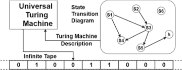
One of the most important properties of a computation system like TMs is that there exists a universal machine that can simulate each machine from its code.

Let us first consider one-tape DTMs with the input alphabet ${0,1}$, the working alphabet ${0,1, \mathrm{~B}}$, the initial state $q_{0}$, and the final state set $\left{q_{1}\right}$, that is, DTMs defined by $\left(Q, q_{0},\left{q_{1}\right},{0,1},{0,1, \mathrm{~B}}, \delta\right)$. Such a TM can be determined by the definition of the transition function $\delta$ only, for $Q$ is assumed to be the set of states appearing in the definition of $\delta$. Let us use the notation $q_{i}, 0 \leq i \leq|Q|-1$, for a state in $Q, X_{j}, j=0,1,2$, for a tape symbol where $X_{0}=0, X_{1}=1$ and $X_{2}=\mathrm{B}$, and $D_{k}, k=0$, lor a moving direction for the tape head where $D_{0}=\mathrm{L}$ and $D_{1}=\mathrm{R}$. For each equation $\delta\left(q_{i}, X_{j}\right)=\left(q_{k}, X_{\ell}, D_{h}\right)$, we encode it by the following string in ${0,1}^{*}$ :
$$
0^{i+1} 10^{j+1} 10^{k+1} 10^{\ell+1} 10^{h+1} .
$$
Assume that there are $m$ equations in the definition of $\delta$. Let code $e_{i}$ be the code of the $i$ th equation. Then we combine the codes for equations together to get the following code for the TM:
$$
\text { code }{1} 11 \text { code }{2} 11 \cdots 11 \text { code }_{m} \text {. }
$$
Note that because different orderings of the equations give different codes, there are $m$ ! equivalent codes for a TM of $m$ equations.

The above coding system is a one-to-many mapping $\phi$ from TMs to ${0,1}^{}$. Each string $x$ in ${0,1}^{}$ encodes at most one TM $\phi^{-1}(x)$. Let us extend $\phi^{-1}$ into a function mapping each string $x \in{0,1}^{}$ to a TM $M$ by mapping each $x$ not encoding a TM to a fixed empty TM $M_{0}$ whose code is $\lambda$ and that rejects all strings. Call this mapping $t$. Observe that $t$ is a mapping from ${0,1}^{}$ to TMs with the following properties:
(i) For every $x \in \Sigma^{*}, t(x)$ represents a TM;
(ii) Every TM is represented by at least one $\iota(x)$; and
(iii) The transition function $\delta$ of the TM $t(x)$ can be easily decoded from the string $x$.

We say a coding system $t$ is an emumeration of one-tape DTMs if $t$ satisfies properties (i) and (ii). In addition, property (iii) means that this enumeration admits a universal Turing machine. In the following, we write $M_{x}$ to mean the TM $\iota(x)$. We assume that $\langle\cdot, \cdot\rangle$ is a pairing function on ${0,1}^{*}$ such that both the function and its inverse are computable in linear time, for instance, $\langle x, y\rangle=0^{|x|} 1 x y$.

数学代写|计算复杂度理论代写Computational complexity theory代考|Diagonalization

Diagonalization is an important proof technique widely used in recursive function theory and complexity theory. One of the earliest applications of diagonalization is Cantor’s proof for the fact that the set of real numbers is not countable. We give a similar proof for the set of functions on ${0,1}^{*}$. A set $S$ is countable (or, enumerable) if there exists a one-one onto mapping from the set of natural numbers to $S$.

Proposition $1.20$ The set of functions from ${0,1}^{}$ to ${0,1}$ is not countable. Proof. Suppose, by way of contradiction, that such a set is countable, that is, it can be represented as $\left{f_{0}, f_{1}, f_{2}, \cdots\right}$. Let $a_{i}$ denote the $i$ th string in ${0,1}^{}$ under the lexicographic ordering. Then we can define a function $f$ as follows: For each $i \geq 0, f\left(a_{i}\right)=1$ if $f_{i}\left(a_{i}\right)=0$ and $f\left(a_{i}\right)=0$ if $f_{i}\left(a_{i}\right)=1$. Clearly, $f$ is a function from ${0,1}^{*}$ to ${0,1}$. However, it is not in the list $f_{0}, f_{1}, f_{2}, \cdots$, because it differs from each $f_{i}$ on at least one input string $a_{i}$. This establishes a contradiction.

An immediate consequence of Proposition $1.20$ is that there exists a noncomputable function from ${0,1}^{}$ to ${0,1}$, because we have just shown that the set of all TMs, and hence the set of all computable functions, is countable. In the following, we use diagonalization to construct directly an undecidable (i.e., nonrecursive) problem: the halting problem. The halting problem is the set $K=\left{x \in{0,1}^{}: M_{x}\right.$ halts on $\left.x\right}$, where $\left{M_{x}\right}$ is an enumeration of TMs.
Theorem $1.21 K$ is r.e. but not recursive.
Proof. The fact that $K$ is r.e. follows immediately from the existence of the universal TM $M_{u}$ (Proposition 1.17). To see that $K$ is not recursive, we note that the complement of a recursive set is also recursive and, hence, r.e. Thus, if $K$ were recursive, then $\bar{K}$ would be r.e. and there would be an integer $y$ such that $M_{y}$ halts on all $x \in \bar{K}$ and does not halt on any $x \in K$. Then, a contradiction could be found when we consider whether or not $y$ itself is in $K$ : if $y \in K$, then $M_{y}$ must not halt on $y$ and it follows from the definition of $K$ that $y \notin K$ and if $y \notin K$, then $M_{y}$ must halt on $y$ and it follows from the definition of $K$ that $y \in K$.

数学代写|计算复杂度理论代写Computational complexity theory代考|Simulation

We study, in this section, the relationship between deterministic and nondeterministic complexity classes, as well as the relationship between time- and space-bounded complexity classes. We show several different simulations of nondeterministic machines by deterministic ones.
Theorem $1.28$ (a) For any fully space-constructible function $f(n) \geq n$,
$$
D T I M E(f(n)) \subseteq N T I M E(f(n)) \subseteq D S P A C E(f(n)) .
$$
(b) For any fully space-constructible function $f(n) \geq \log n$,
$$
D S P A C E(f(n)) \subseteq N S P A C E(f(n)) \subseteq \bigcup_{c>0} D T I M E\left(2^{f(n)}\right) .
$$
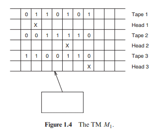
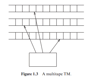
Proof. (a): The relation DTIME(f(n)) $\subseteq \operatorname{NTIME}(f(n))$ follows immediately from the fact that DTMs are just a subclass of NTMs. For the relation $N T I M E(f(n)) \subseteq D S P A C E(f(n))$, we recall the simulation of an NTM $M$ by a DTM $M_{1}$ as described in Theorem 1.9. Suppose that $M$ has time complexity bounded by $f(n)$; then $M_{1}$ needs to simulate $M$ for at most $f(n)$ moves. That is, we restrict $M_{1}$ to only execute the first $\sum_{j=1}^{f(n)} k^{i}$ stages such that the strings written in tape 2 are at most $f(n)$ symbols long. As $f(n)$ is fully space constructible, this restriction can be done by first marking off $f(n)$ squares on tape 2 . It is clear that such a restricted simulation works within space $f(n)$.
$\mathrm{~ ( b ) : ~ A g a i n , ~ D S P A C E ( f ( n ) ) ~}$ $N S P A C E(f(n)) \subseteq \bigcup_{c>0} D T I M E\left(2^{c f(n)}\right)$, assume that $M$ is an NTM with the space bound $f(n)$. We are going to construct a DTM $M_{1}$ to simulate $M$ in time $2^{c f(n)}$ for some $c>0$. As $M$ uses only space $f(n)$, there is a constant $c_{1}>0$ such that the shortest accepting computation for each $x \in L(M)$ is of length $\leq 2^{c_{1} f(|x|)}$. Thus, the machine $M_{1}$ needs only to simulate $M(x)$ for, at most, $2^{c_{1} f(n)}$ moves. However, $M$ is a nondeterministic machine and so its computation tree of depth $2^{c_{1} f(n)}$ could have $2^{20(\text { a }}$ ) naive simulation as (a) above takes too much time.

To reduce the deterministic simulation time, we notice that this computation tree, although of size $2^{2^{2 \varphi(m))}}$, has at most $2^{O(f(n))}$ different configurations: Each configuration is determined by at most $f(n)$ tape symbols on the work tape, one of $f(n)$ positions for the work tape head,one of $n$ positions for the input tape head, and one of $r$ positions for states, where $r$ is a constant. Thus, the total number of possible configurations of $M(x)$ is $2^{O(f(n))} \cdot f(n) \cdot n \cdot r=2^{O(f(n))}$. (Note that $f(n) \geq \log n$ implies $\left.n \leq 2^{f(n)}\right)$

计算复杂度理论代考

像 TM 这样的计算系统最重要的属性之一是存在一个通用机器，可以根据其代码模拟每台机器。

让我们首先考虑输入字母表的单磁带 DTM0,1, 工作字母表0,1, 乙, 初始状态q0, 和最终状态集\left{q_{1}\right}\left{q_{1}\right}，即 DTM 定义为\left(Q, q_{0},\left{q_{1}\right},{0,1},{0,1, \mathrm{~B}}, \delta\right)\left(Q, q_{0},\left{q_{1}\right},{0,1},{0,1, \mathrm{~B}}, \delta\right). 这样的 TM 可以通过转换函数的定义来确定d仅适用于问被假定为出现在定义中的状态集d. 让我们使用符号q一世,0≤一世≤|问|−1, 对于一个状态问,Xj,j=0,1,2，对于磁带符号，其中X0=0,X1=1和X2=乙，和Dķ,ķ=0，或磁带头的移动方向，其中D0=大号和D1=R. 对于每个方程d(q一世,Xj)=(qķ,Xℓ,DH)，我们通过以下字符串对其进行编码0,1∗ :

0一世+110j+110ķ+110ℓ+110H+1.
假设有米定义中的方程d. 让代码和一世成为代码一世方程。然后我们将方程的代码组合在一起，得到以下 TM 代码：

代码 111 代码 211⋯11 代码米.
请注意，由于方程的不同排序给出不同的代码，所以有米！TM 的等效代码米方程。

上述编码系统是一对多的映射φ从 TM 到0,1. 每个字符串X在0,1最多编码一个 TMφ−1(X). 让我们扩展φ−1到一个函数映射每个字符串X∈0,1到 TM米通过映射每个X不将 TM 编码为固定的空 TM米0谁的代码是λ并且拒绝所有字符串。调用此映射吨. 请注意吨是来自的映射0,1具有以下属性的 TM：
(i) 对于每个X∈Σ∗,吨(X)代表 TM；
(ii) 每个 TM 至少由一个代表我(X); (
iii) 过渡函数dTM的吨(X)可以很容易地从字符串中解码X.

我们说一个编码系统吨是单磁带 DTM 的枚举，如果吨满足性质 (i) 和 (ii)。此外，性质（iii）意味着这个枚举承认一个通用的图灵机。下面，我们写米X意思是 TM我(X). 我们假设⟨⋅,⋅⟩是一个配对函数0,1∗使得函数及其逆函数都可以在线性时间内计算，例如，⟨X,是⟩=0|X|1X是.

数学代写|计算复杂度理论代写Computational complexity theory代考|Diagonalization

对角化是递归函数理论和复杂性理论中广泛使用的重要证明技术。对角化最早的应用之一是康托尔证明实数集不可数的事实。我们对函数集给出了类似的证明0,1∗. 一套小号是可数的（或者，可枚举的），如果存在从自然数集到的一对一映射到小号.

主张1.20函数集来自0,1至0,1不可数。证明。假设，通过矛盾的方式，这样一个集合是可数的，也就是说，它可以表示为\left{f_{0}, f_{1}, f_{2}, \cdots\right}\left{f_{0}, f_{1}, f_{2}, \cdots\right}. 让一个一世表示一世第一个字符串0,1在字典顺序下。然后我们可以定义一个函数F如下：对于每个一世≥0,F(一个一世)=1如果F一世(一个一世)=0和F(一个一世)=0如果F一世(一个一世)=1. 清楚地，F是一个函数0,1∗至0,1. 但是，它不在列表中F0,F1,F2,⋯，因为它不同于每个F一世在至少一个输入字符串上一个一世. 这就产生了矛盾。

命题的直接后果1.20是存在一个不可计算的函数0,1至0,1，因为我们刚刚证明了所有 TM 的集合，以及所有可计算函数的集合，都是可数的。下面，我们使用对角化直接构造一个不可判定的（即非递归的）问题：停机问题。停机问题是集合K=\left{x \in{0,1}^{}: M_{x}\right.$ 停在 $\left.x\right}K=\left{x \in{0,1}^{}: M_{x}\right.$ 停在 $\left.x\right}，在哪里\left{M_{x}\right}\left{M_{x}\right}是 TM 的枚举。
定理1.21ķ是 re 但不是递归的。
证明。事实是ķ是从普遍 TM 的存在中直接得出的米在（提案 1.17）。看到那个ķ不是递归的，我们注意到递归集的补集也是递归的，因此， re 因此，如果ķ是递归的，那么ķ¯将是 re 并且会有一个整数是这样米是停在所有X∈ķ¯并且不会停止任何X∈ķ. 那么，当我们考虑是否是本身在ķ：如果是∈ķ，然后米是不能停在是并且它遵循以下定义ķ那是∉ķ而如果是∉ķ，然后米是必须停止是并且它遵循以下定义ķ那是∈ķ.

数学代写|计算复杂度理论代写Computational complexity theory代考|Simulation

在本节中，我们研究确定性和非确定性复杂性类之间的关系，以及时间和空间受限复杂性类之间的关系。我们通过确定性机器展示了几种不同的非确定性机器模拟。
定理1.28(a) 对于任何完全空间可构造函数F(n)≥n,

D吨我米和(F(n))⊆ñ吨我米和(F(n))⊆D小号磷一个C和(F(n)).
(b) 对于任何完全空间可构造函数F(n)≥日志⁡n,

D小号磷一个C和(F(n))⊆ñ小号磷一个C和(F(n))⊆⋃C>0D吨我米和(2F(n)).
证明。(a): 关系 DTIME(f(n))⊆新时代⁡(F(n))紧接着 DTM 只是 NTM 的一个子类这一事实。对于关系ñ吨我米和(F(n))⊆D小号磷一个C和(F(n))，我们回忆一下 NTM 的模拟米通过 DTM米1如定理 1.9 所述。假设米时间复杂度为F(n); 然后米1需要模拟米最多为F(n)移动。也就是说，我们限制米1只执行第一个∑j=1F(n)ķ一世阶段，使得写在磁带 2 中的字符串最多F(n)符号长。作为F(n)是完全空间可构造的，这个限制可以通过首先标记F(n)磁带上的正方形 2 。很明显，这种受限的模拟在空间内有效F(n).
(b): 一个G一个一世n, D小号磷一个C和(F(n)) ñ小号磷一个C和(F(n))⊆⋃C>0D吨我米和(2CF(n))，假使，假设米是一个有空间限制的 NTMF(n). 我们将构建一个 DTM米1模拟米及时2CF(n)对于一些C>0. 作为米仅使用空间F(n), 有一个常数C1>0这样每个的最短接受计算X∈大号(米)有长度≤2C1F(|X|). 因此，机米1只需要模拟米(X)因为，至多，2C1F(n)移动。然而，米是一个不确定的机器，因此它的深度计算树2C1F(n)本来可以220( 一个 ) 上面 (a) 的幼稚模拟需要太多时间。

为了减少确定性模拟时间，我们注意到这个计算树，虽然大小222披(米)), 最多有2○(F(n))不同的配置：每个配置最多由F(n)工作磁带上的磁带符号，其中之一F(n)工作磁带头的位置，其中之一n输入磁带头的位置，以及其中之一r各州的职位，其中r是一个常数。因此，可能的配置总数米(X)是2○(F(n))⋅F(n)⋅n⋅r=2○(F(n)). （注意F(n)≥日志⁡n暗示n≤2F(n))

数学代写|计算复杂度理论代写Computational complexity theory代考请认准statistics-lab™

统计代写请认准statistics-lab™. statistics-lab™为您的留学生涯保驾护航。

金融工程代写

金融工程是使用数学技术来解决金融问题。金融工程使用计算机科学、统计学、经济学和应用数学领域的工具和知识来解决当前的金融问题，以及设计新的和创新的金融产品。

非参数统计代写

非参数统计指的是一种统计方法，其中不假设数据来自于由少数参数决定的规定模型；这种模型的例子包括正态分布模型和线性回归模型。

广义线性模型代考

广义线性模型（GLM）归属统计学领域，是一种应用灵活的线性回归模型。该模型允许因变量的偏差分布有除了正态分布之外的其它分布。

术语广义线性模型（GLM）通常是指给定连续和/或分类预测因素的连续响应变量的常规线性回归模型。它包括多元线性回归，以及方差分析和方差分析（仅含固定效应）。

有限元方法代写

有限元方法（FEM）是一种流行的方法，用于数值解决工程和数学建模中出现的微分方程。典型的问题领域包括结构分析、传热、流体流动、质量运输和电磁势等传统领域。

有限元是一种通用的数值方法，用于解决两个或三个空间变量的偏微分方程（即一些边界值问题）。为了解决一个问题，有限元将一个大系统细分为更小、更简单的部分，称为有限元。这是通过在空间维度上的特定空间离散化来实现的，它是通过构建对象的网格来实现的：用于求解的数值域，它有有限数量的点。边界值问题的有限元方法表述最终导致一个代数方程组。该方法在域上对未知函数进行逼近。[1] 然后将模拟这些有限元的简单方程组合成一个更大的方程系统，以模拟整个问题。然后，有限元通过变化微积分使相关的误差函数最小化来逼近一个解决方案。

tatistics-lab作为专业的留学生服务机构，多年来已为美国、英国、加拿大、澳洲等留学热门地的学生提供专业的学术服务，包括但不限于Essay代写，Assignment代写，Dissertation代写，Report代写，小组作业代写，Proposal代写，Paper代写，Presentation代写，计算机作业代写，论文修改和润色，网课代做，exam代考等等。写作范围涵盖高中，本科，研究生等海外留学全阶段，辐射金融，经济学，会计学，审计学，管理学等全球99%专业科目。写作团队既有专业英语母语作者，也有海外名校硕博留学生，每位写作老师都拥有过硬的语言能力，专业的学科背景和学术写作经验。我们承诺100%原创，100%专业，100%准时，100%满意。

随机分析代写

随机微积分是数学的一个分支，对随机过程进行操作。它允许为随机过程的积分定义一个关于随机过程的一致的积分理论。这个领域是由日本数学家伊藤清在第二次世界大战期间创建并开始的。

时间序列分析代写

随机过程，是依赖于参数的一组随机变量的全体，参数通常是时间。随机变量是随机现象的数量表现，其时间序列是一组按照时间发生先后顺序进行排列的数据点序列。通常一组时间序列的时间间隔为一恒定值（如1秒，5分钟，12小时，7天，1年），因此时间序列可以作为离散时间数据进行分析处理。研究时间序列数据的意义在于现实中，往往需要研究某个事物其随时间发展变化的规律。这就需要通过研究该事物过去发展的历史记录，以得到其自身发展的规律。

回归分析代写

多元回归分析渐进（Multiple Regression Analysis Asymptotics）属于计量经济学领域，主要是一种数学上的统计分析方法，可以分析复杂情况下各影响因素的数学关系，在自然科学、社会和经济学等多个领域内应用广泛。

MATLAB代写

MATLAB 是一种用于技术计算的高性能语言。它将计算、可视化和编程集成在一个易于使用的环境中，其中问题和解决方案以熟悉的数学符号表示。典型用途包括：数学和计算算法开发建模、仿真和原型制作数据分析、探索和可视化科学和工程图形应用程序开发，包括图形用户界面构建MATLAB 是一个交互式系统，其基本数据元素是一个不需要维度的数组。这使您可以解决许多技术计算问题，尤其是那些具有矩阵和向量公式的问题，而只需用 C 或 Fortran 等标量非交互式语言编写程序所需的时间的一小部分。MATLAB 名称代表矩阵实验室。MATLAB 最初的编写目的是提供对由 LINPACK 和 EISPACK 项目开发的矩阵软件的轻松访问，这两个项目共同代表了矩阵计算软件的最新技术。MATLAB 经过多年的发展，得到了许多用户的投入。在大学环境中，它是数学、工程和科学入门和高级课程的标准教学工具。在工业领域，MATLAB 是高效研究、开发和分析的首选工具。MATLAB 具有一系列称为工具箱的特定于应用程序的解决方案。对于大多数 MATLAB 用户来说非常重要，工具箱允许您学习和应用专业技术。工具箱是 MATLAB 函数（M 文件）的综合集合，可扩展 MATLAB 环境以解决特定类别的问题。可用工具箱的领域包括信号处理、控制系统、神经网络、模糊逻辑、小波、仿真等。

R语言代写	问卷设计与分析代写
PYTHON代写	回归分析与线性模型代写
MATLAB代写	方差分析与试验设计代写
STATA代写	机器学习/统计学习代写
SPSS代写	计量经济学代写
EVIEWS代写	时间序列分析代写
EXCEL代写	深度学习代写
SQL代写	各种数据建模与可视化代写

数学代写|计算复杂度理论代写Computational complexity theory代考|Models of Computation and Complexity Classes

Posted on 2022年6月24日2022年6月24日 by statistics-lab

如果你也在怎样代写计算复杂度理论Computational complexity theory这个学科遇到相关的难题，请随时右上角联系我们的24/7代写客服。

我们提供的计算复杂度理论Computational complexity theory及其相关学科的代写，服务范围广, 其中包括但不限于:

Statistical Inference 统计推断
Statistical Computing 统计计算
Advanced Probability Theory 高等概率论
Advanced Mathematical Statistics 高等数理统计学
(Generalized) Linear Models 广义线性模型
Statistical Machine Learning 统计机器学习
Longitudinal Data Analysis 纵向数据分析
Foundations of Data Science 数据科学基础

数学代写|计算复杂度理论代写Computational complexity theory代考|Models of Computation and Complexity Classes

数学代写|计算复杂度理论代写Computational complexity theory代考|Strings, Coding, and Boolean Functions

Our basic data structure is a string. All other data structures are to be encoded and represented by strings. A string is a finite sequence of symbols. For instance, the word string is a string over the symbols of English letters; the arithmetic expression ” $3+4-5$ ” is a string over symbols $3,4,5,+$, and -. Thus, to describe a string, we must specify the set of symbols to occur in that string. We call a finite set of symbols to be used to define strings an alphabet. Note that not every finite set can be an alphabet. A finite set $S$ can be an alphabet if and only if the following condition holds.

Property 1.1 Two finite sequences of elements in $S$ are identical if and only if the elements in the two sequences are identical respectively in ordering.
For example, ${0,1}$ and ${00,01}$ are alphabets, but ${1,11}$ is not an alphabet because 11 can be formed by either 11 or ( 1 and 1$)$.

Assume that $\Sigma$ is an alphabet. A set of strings over the alphabet $\Sigma$ is called a language. A collection of languages is called a language class, or simply a class.

There is a fundamental operation on strings. The concatenation of two strings $x$ and $y$ is the string $x y$. The concatenation follows associative law, that is, $x(y z)=(x y) z$. Moreover, $\lambda x=x \lambda=x$. Thus, all strings over an alphabet form a monoid under concatenation. ${ }^{1}$ We denote $x^{0}=\lambda$ and $x^{n}=x x^{n-1}$ for $n \geq 1$.

The concatenation operation on strings can be extended to languages. The concatenation of two languages $A$ and $B$ is the language $A B={a b$ : $a \in A, b \in B}$. We also denote $A^{0}={\lambda}$ and $A^{n}=A A^{n-1}$ for $n \geq 1$. In addition, we define $A^{}=\bigcup_{i=0}^{\infty} A^{i}$. The language $A^{}$ is called the Kleene closure of $A$. The Kleene closure of an alphabet is the set of all strings over the alphabet.

数学代写|计算复杂度理论代写Computational complexity theory代考|Deterministic Turing Machines

Turing machines (TMs) are simple and yet powerful enough computational models. Almost all reasonable general-purpose computational models have been known to be equivalent to TMs, in the sense that they define the same class of computable functions. There are many variations of TMs studied in literature. We are going to introduce, in this section,

the simplest model of TMs, namely, the deterministic Turing machine (DTM). Another model, the nondeterministic Turing machine (NTM), is to be defined in the next section. Other generalized TM models, such as deterministic and nondeterministic oracle TMs, will be defined in later chapters. In addition, we will introduce in Part II other nonuniform computational models which are not equivalent to TMs.

A deterministic (one-tape) TM (DTM) consists of two basic units: the control unit and the memory unit. The control unit contains a finite number of states. The memory unit is a tape that extends infinitely to both ends. The tape is divided into an infinite number of tape squares (or, tape cells). Each tape square stores one of a finite number of tape symbols. The communication between the control unit and the tape is through a readlwrite tape head that scans a tape square at a time (See Figure 1.1).
A normal move of a TM consists of the following actions:
(1) Reading the tape symbol from the tape square currently scanned by the tape head;
(2) Writing a new tape symbol on the tape square currently scanned by the tape head;
(3) Moving the tape head to the right or left of the current square; and
(4) Changing to a new control state.

数学代写|计算复杂度理论代写Computational complexity theory代考|Nondeterministic Turing Machines

The TMs we defined in the last section are deterministic, because from each configuration of a machine there is at most one move to make, and hence, there is at most one next configuration. If we allow more than one moves for some configurations, and hence those configurations have more than one next configurations, then the machine is called a nondeterministic Turing machine (NTM).

Formally, an NTM $M$ is defined by the following information: states $Q$; initial state $q_{0}$; accepting states $F$; input symbols $\Sigma$; tape symbols $\Gamma$, including the blank symbol $\mathrm{B}$; and the transition relation $\Delta$. All information except the transition relation $\Delta$ is defined in the same form as a DTM. The transition relation $\Delta$ is a subset of $(Q-F) \times \Gamma \times Q \times \Gamma \times$ ${\mathrm{L}, \mathrm{R}}$. Each quintuple $\left(q_{1}, s_{1}, q_{2}, s_{2}, D\right)$ in $\Delta$ indicates that one of the possible moves of $M$, when it is in state $q_{1}$ and scanning symbol $s_{1}$, is to change the current state to $q_{2}$, to overwrite symbol $s_{1}$ by $s_{2}$, and to move the tape head to the direction $D$.

The computation of an NTM can be defined similar to that of a DTM. First, we consider a way of restricting an NTM to a DTM. Let $M$ be an NTM defined by $\left(Q, q_{0}, F, \Sigma, \Gamma, \Delta\right)$ as above. We say $M_{1}$ is a restricted DTM of $M$ if $M_{1}$ has the same components $Q, q_{0}, F, \Sigma, \Gamma$ as $M$ and it has a transition function $\delta_{1}$ that is a subrelation of $\Delta$ satisfying the property that for each $q_{1} \in Q$ and $s_{1} \in \Gamma$, there is at most one triple $\left(q_{2}, s_{2}, D\right)$, $D \in{\mathrm{L}, \mathrm{R}}$, such that $\left(q_{1}, s_{1}, q_{2}, s_{2}, D\right) \in \delta_{1}$. Now we can define the notion of the next configurations of an NTM easily: For each configuration $\alpha=$ $\left(q_{1}, x_{1}, y_{1}\right)$ of $M$, we let $\vdash_{M}(\alpha)$ be the set of all configurations $\beta$ such that $\alpha \vdash_{M_{1}} \beta$ for some restricted DTM $M_{1}$ of $M$. We write $\alpha \vdash_{M} \beta$ if $\beta \in \vdash_{M}(\alpha)$. As each configuration of $M$ may have more than one next configurations, the computation of an NTM on an input $w$ is, in general, a computation tree rather than a single computation path (as it is in the case of DTMs). In the computation tree, each node is a configuration $\alpha$ and all its next configurations are its children. The root of the tree is the initial configuration.

We say an NTM $M$ halts on an input string $w \in \Sigma^{*}$ if there exists a finite sequence of configurations $\alpha_{0}, \alpha_{1}, \ldots, \alpha_{n}$ such that
(1) $\alpha_{0}=\left(q_{0}, \lambda, w\right)$;
(2) $\alpha_{i} \vdash_{M} \alpha_{i+1}$ for all $i=0,1, \ldots, n-1$; and
(3) $\vdash_{M}\left(\alpha_{n}\right)$ is undefined (i.e., it is an empty set).

计算复杂度理论代考

数学代写|计算复杂度理论代写Computational complexity theory代考|Strings, Coding, and Boolean Functions

我们的基本数据结构是一个字符串。所有其他数据结构都将由字符串编码和表示。字符串是有限的符号序列。例如，字串是英文字母符号之上的字符串；算术表达式”3+4−5” 是符号上的字符串3,4,5,+，和 -。因此，要描述一个字符串，我们必须指定该字符串中出现的符号集。我们将用于定义字符串的有限符号集称为字母表。请注意，并非每个有限集都可以是字母表。有限集小号当且仅当以下条件成立时，它才能是字母表。

性质 1.1 中的两个有限元素序列小号当且仅当两个序列中的元素在顺序上分别相同时，它们是相同的。
例如，0,1和00,01是字母，但是1,11不是字母，因为 11 可以由 11 或 ( 1 和 1).

假使，假设Σ是一个字母。字母表上的一组字符串Σ被称为语言。语言的集合称为语言类，或简称为类。

字符串的长度X是字符串中的符号数X，表示为|X|. 例如，∣细绳∣=6和|3+4−5|=5. 为方便起见，我们允许字符串不包含符号。这样的字符串称为空字符串，记为λ. 所以，|λ|=0. （符号|⋅|也用于集合。如果小号是一个有限集，我们写|小号|来表示它的基数。）

对字符串有一个基本的操作。两个字符串的连接X和是是字符串X是. 串联遵循结合律，即X(是和)=(X是)和. 而且，λX=Xλ=X. 因此，字母表上的所有字符串在连接下形成一个幺半群。1我们表示X0=λ和Xn=XXn−1为了n≥1.

字符串的连接操作可以扩展到语言。两种语言的连接一个和乙是语言一个乙=一个b$:$一个∈一个,b∈乙. 我们还表示一个0=λ和一个n=一个一个n−1为了n≥1. 此外，我们定义一个=⋃一世=0∞一个一世. 语言一个称为 Kleene 闭包一个. 字母表的 Kleene 闭包是字母表上所有字符串的集合。

数学代写|计算复杂度理论代写Computational complexity theory代考|Deterministic Turing Machines

图灵机 (TM) 是简单但足够强大的计算模型。众所周知，几乎所有合理的通用计算模型都等同于 TM，因为它们定义了同一类可计算函数。文献中研究了许多不同的 TM。我们将在本节中介绍，

最简单的 TM 模型，即确定性图灵机 (DTM)。另一个模型，非确定性图灵机 (NTM)，将在下一节中定义。其他通用 TM 模型，例如确定性和非确定性预言机 TM，将在后面的章节中定义。此外，我们将在第二部分介绍其他不等同于 TM 的非均匀计算模型。

确定性（单磁带）TM (DTM) 由两个基本单元组成：控制单元和存储单元。控制单元包含有限数量的状态。内存单元是无限延伸到两端的磁带。磁带被分成无数个磁带方格（或磁带单元）。每个磁带方存储有限数量的磁带符号之一。控制单元和磁带之间的通信是通过一个读写磁带头进行的，该磁头一次扫描一个磁带方格（见图 1.1）。
一个 TM 的正常移动由以下动作组成：
(1) 从磁带头当前扫描的磁带方格中读取磁带符号；
(2)在磁带头当前扫描的磁带方格上写入一个新的磁带符号；
(3) 将磁带头移动到当前方格的右侧或左侧；(
4) 转变为新的控制状态。

数学代写|计算复杂度理论代写Computational complexity theory代考|Nondeterministic Turing Machines

我们在上一节中定义的 TM 是确定性的，因为机器的每个配置最多有一个动作要做，因此最多有一个下一个配置。如果我们允许对某些配置进行多次移动，因此这些配置具有多个下一个配置，则该机器称为非确定性图灵机 (NTM)。

正式地，一个 NTM米由以下信息定义：状态问; 初始状态q0; 接受状态F; 输入符号Σ; 磁带符号Γ, 包括空白符号乙; 和过渡关系Δ. 除转移关系外的所有信息Δ以与 DTM 相同的形式定义。过渡关系Δ是的一个子集(问−F)×Γ×问×Γ× 大号,R. 每个五重奏(q1,s1,q2,s2,D)在Δ表示可能的移动之一米, 当它处于状态时q1和扫描符号s1, 是将当前状态更改为q2, 覆盖符号s1经过s2, 并将磁带头移动到方向D.

NTM 的计算可以定义为类似于 DTM 的计算。首先，我们考虑一种将 NTM 限制为 DTM 的方法。让米是由以下定义的 NTM(问,q0,F,Σ,Γ,Δ)如上。我们说米1是一个受限制的 DTM米如果米1具有相同的组件问,q0,F,Σ,Γ作为米并且有过渡功能d1这是一个子关系Δ满足对于每个q1∈问和s1∈Γ, 最多有一个三元组(q2,s2,D), D∈大号,R, 这样(q1,s1,q2,s2,D)∈d1. 现在我们可以轻松定义 NTM 的下一个配置的概念：对于每个配置一个= (q1,X1,是1)的米，我们让⊢米(一个)是所有配置的集合b这样一个⊢米1b对于一些受限的 DTM米1的米. 我们写一个⊢米b如果b∈⊢米(一个). 作为每个配置米可能有多个下一个配置，在输入上计算 NTM在通常，它是一个计算树，而不是单个计算路径（就像在 DTM 的情况下一样）。在计算树中，每个节点都是一个配置一个它的所有下一个配置都是它的孩子。树的根是初始配置。

我们说 NTM米在输入字符串上停止在∈Σ∗如果存在有限的配置序列一个0,一个1,…,一个n这样
(1)一个0=(q0,λ,在);
(2) 一个一世⊢米一个一世+1对所有人一世=0,1,…,n−1; (
3)⊢米(一个n)是未定义的（即，它是一个空集）。

统计代写请认准statistics-lab™. statistics-lab™为您的留学生涯保驾护航。

金融工程代写

非参数统计代写

非参数统计指的是一种统计方法，其中不假设数据来自于由少数参数决定的规定模型；这种模型的例子包括正态分布模型和线性回归模型。

广义线性模型代考

广义线性模型（GLM）归属统计学领域，是一种应用灵活的线性回归模型。该模型允许因变量的偏差分布有除了正态分布之外的其它分布。

有限元方法代写

随机分析代写

时间序列分析代写

回归分析代写

MATLAB代写

R语言代写	问卷设计与分析代写
PYTHON代写	回归分析与线性模型代写
MATLAB代写	方差分析与试验设计代写
STATA代写	机器学习/统计学习代写
SPSS代写	计量经济学代写
EVIEWS代写	时间序列分析代写
EXCEL代写	深度学习代写
SQL代写	各种数据建模与可视化代写

数学代写|计算复杂度理论代写Computational complexity theory代考|Order-Disorder Phase Transitions in the Agent Population

Posted on 2022年6月6日2022年6月6日 by statistics-lab

如果你也在怎样代写计算复杂度理论Computational complexity theory这个学科遇到相关的难题，请随时右上角联系我们的24/7代写客服。

我们提供的计算复杂度理论Computational complexity theory及其相关学科的代写，服务范围广, 其中包括但不限于:

Statistical Inference 统计推断
Statistical Computing 统计计算
Advanced Probability Theory 高等概率论
Advanced Mathematical Statistics 高等数理统计学
(Generalized) Linear Models 广义线性模型
Statistical Machine Learning 统计机器学习
Longitudinal Data Analysis 纵向数据分析
Foundations of Data Science 数据科学基础

数学代写|计算复杂度理论代写Computational complexity theory代考|Order-Disorder Phase Transitions in the Agent Population

As discussed before, in the “information domain,” we can study the system by mapping strategies to spins. In addition, we can map the difference between winning

probabilities, of cooperators and defectors, to an external magnetic field: $h=$ $p_{c}^{b}-p_{d^{b}}^{b}$. In doing so, by the Landau theory, we can analytically identify an orderdisorder phase transition. Notably, we analyze the free energy $F$ of the spin system on varying the control parameter $m$ (corresponding to the magnetization $M$ )
$$
F(m)=-h m \pm \frac{m^{2}}{2}+\frac{m^{4}}{4}
$$
where the sign of the second term depends on the temperature, i.e., positive for $T_{s}>$ $T_{c}$ and negative for $T_{s}<T_{c}$; we remind that $T_{c}$ represents the temperature beyond which it is not possible to play the PD due to the high particle speed (according to our assumption). For the sake of clarity, we want to emphasize that the free energy is introduced in order to evaluate the nature of the final equilibrium achieved by the system. In particular, looking for the minima of $F$ allows to investigate if our population reaches the Nash equilibrium, or different configurations (e.g., full cooperation). Figure $3.5$ shows a pictorial representation of the phase transitions that can occur in our system, on varying $T_{s}$ and the external field $h$. Then, the constraints related to the average speed of particles, and to the distance between each group and the permeable wall, can be in principle relaxed, as we can imagine to extend this description to a wider system with several groups, where agents are uniformly distributed in the whole space. Now, it is worth to highlight that our results are completely in agreement with those achieved by authors who studied the role of motion in the PD and in addition are able to explain why clusters of cooperators emerge in these conditions. At the same time, we remind that, in this model, agents are “memory-aware,” while usually investigations consider agents that reset their payoff at each step.

数学代写|计算复杂度理论代写Computational complexity theory代考|The Role of the Temperature in the Spatial Public Goods Game

In this section, we aim to analyze the role of the temperature in the spatial PGG. Before to proceed, it is important to remind the reader that, in this section, the terms “temperature” and “noise” refer to the same concept. As discussed in Chap. 1 , the dynamics of this game are affected by a number of parameters and processes, namely, the topology of interactions among the agents, the synergy factor, and the strategy revision phase. We remind that the latter is a process that allows agents to change their strategy. Notably, rational agents tend to imitate richer neighbors, in order to increase the probability to maximize their payoff. By implementing a stochastic revision process, it is possible to control the level of noise in the system, so that even irrational updates may be observed. In particular, we study the effect of noise on the macroscopic behavior of a finite structured population. We consider both the case of a homogeneous population, where the noise in the system is controlled by tuning a parameter representing the level of stochasticity in the strategy revision phase, and a heterogeneous population composed of a variable proportion of rational and irrational agents. In both cases numerical investigations show that the PGG has a very rich behavior, which strongly depends on the amount of noise in the system and on the value of the synergy factor. In doing so, we aim to provide a description of the PGG by the lens of statistical physics, focusing in particular on the impact of noise in the population dynamics. Saying that rational agents are those that tend to imitate their richer neighbors, we can state that irrational agents are those that randomly change their strategy. In the case of a homogeneous population, the intensity of noise in the system is controlled by tuning the level of stochasticity of all agents during the SRP, by means of a global parameter (indicated by $K$ ) that represents the noise/temperature. Instead, in the case of a heterogeneous population, the noise is controlled by tuning the density of irrational agents in the population. Results indicate that tuning the level of noise to interpolate between configurations where agents fully utilize payoff information (low noise) to those where they behave at random (high noise) strongly affects the macroscopic behavior of a population.

数学代写|计算复杂度理论代写Computational complexity theory代考|Model

In the case of well-mixed populations of infinite size, the behavior of the system can be predicted as a function of the synergy factor $r$ by studying the related Nash equilibria. In particular, when agents play in groups of $G$ players, two different absorbing states appear separated at a critical point $r_{\mathrm{wm}}=G$. The population falls into full defection for $rr_{\mathrm{wm}}$. Conversely, when agents are arranged in the nodes of a network, surprisingly some cooperators can survive for values of $r$ lower than $r_{\text {wm }}$. This effect, discussed in Chap. 1 , is known as network reciprocity. At the same time, the network structure allows a limited number of defectors to survive also beyond $r=r_{\mathrm{wm}}$. We refer to the two critical values of $r$ at which cooperators first appear and defectors eventually disappear from the population, respectively, as $r_{c 1}$ and $r_{c 2}$. It is worth mentioning that most investigations in EGT are performed by numerical simulations, and an analytical definition of the critical thresholds (i.e., $r_{c 1}$ and $r_{c 2}$ ) identified in networked topologies is missing. As a result, when studying EGT models by arranging agents in different spaces, the values of critical thresholds are achieved by Monte Carlo simulations (see Chap. 2). In a networked population, depending on the values of $r$ and on how agents are allowed to update their strategy, it is possible to observe different regimes: two ordered equilibrium absorbing phases, where only one strategy survives (either cooperation or defection), and an active but macroscopically stable disordered phase corresponding to the coexistence between the two species/strategies.

计算复杂度理论代考

数学代写|计算复杂度理论代写Computational complexity theory代考|Order-Disorder Phase Transitions in the Agent Population

如前所述，在“信息域”中，我们可以通过将策略映射到自旋来研究系统。此外，我们可以映射获胜之间的差异

合作者和叛逃者对外部磁场的概率：H= pCb−pdbb. 这样做，通过朗道理论，我们可以分析地识别有序无序相变。值得注意的是，我们分析了自由能F改变控制参数的自旋系统米（对应于磁化米 )

F(米)=−H米±米22+米44
其中第二项的符号取决于温度，即，正吨s> 吨C和消极的吨s<吨C; 我们提醒您吨C表示由于高粒子速度（根据我们的假设）而无法播放 PD 的温度。为了清楚起见，我们想强调引入自由能是为了评估系统达到的最终平衡的性质。特别是，寻找最小值F允许调查我们的人口是否达到纳什均衡或不同的配置（例如，完全合作）。数字3.5显示了我们系统中可能发生的相变的图形表示，在不同的吨s和外场H. 然后，原则上可以放宽与粒子平均速度以及每组与可渗透壁之间的距离相关的约束，正如我们可以想象将这种描述扩展到具有多个组的更广泛的系统，其中代理均匀分布在整个空间。现在，值得强调的是，我们的结果与研究运动在 PD 中的作用的作者所取得的结果完全一致，此外还能够解释为什么在这些条件下会出现合作者集群。同时，我们提醒，在这个模型中，代理人是“记忆感知的”，而通常调查考虑代理人在每一步重置他们的收益。

数学代写|计算复杂度理论代写Computational complexity theory代考|The Role of the Temperature in the Spatial Public Goods Game

在本节中，我们旨在分析温度在空间 PGG 中的作用。在继续之前，重要的是要提醒读者，在本节中，术语“温度”和“噪声”指的是同一个概念。如第 1 章所述。如图 1 所示，该博弈的动态受到许多参数和过程的影响，即代理之间交互的拓扑、协同因素和策略修订阶段。我们提醒，后者是一个允许代理人改变策略的过程。值得注意的是，理性的代理人倾向于模仿富裕的邻居，以增加最大化其收益的可能性。通过实施随机修订过程，可以控制系统中的噪声水平，从而甚至可以观察到不合理的更新。尤其是，我们研究了噪声对有限结构化种群宏观行为的影响。我们考虑了同质总体的情况，其中系统中的噪声通过调整代表策略修订阶段随机性水平的参数来控制，以及由可变比例的理性和非理性代理组成的异质总体。在这两种情况下，数值研究表明 PGG 具有非常丰富的行为，这在很大程度上取决于系统中的噪声量和协同因子的值。在此过程中，我们旨在通过统计物理学的视角提供对 PGG 的描述，特别关注噪声对种群动态的影响。说理性的代理人是那些倾向于模仿他们更富有的邻居的人，我们可以说，非理性代理人是那些随机改变策略的代理人。在同质群体的情况下，系统中的噪声强度是通过调整 SRP 期间所有代理的随机性水平来控制的，通过全局参数（表示为ķ) 表示噪声/温度。相反，在异质人口的情况下，噪声是通过调整人口中非理性代理的密度来控制的。结果表明，调整噪声水平以在代理充分利用收益信息（低噪声）与随机行为（高噪声）的配置之间进行插值，会强烈影响群体的宏观行为。

数学代写|计算复杂度理论代写Computational complexity theory代考|Model

在无限大小的混合良好的群体的情况下，系统的行为可以预测为协同因子的函数r通过研究相关的纳什均衡。特别是，当特工成群结队地玩耍时G玩家，两种不同的吸收状态在临界点出现分离r在米=G. 人口全面叛逃rr在米. 相反，当代理被安排在网络的节点中时，令人惊讶的是，一些合作者可以生存r低于rwm . 这种影响，在第 1 章中讨论。1 ，称为网络互惠。同时，网络结构允许有限数量的叛逃者生存r=r在米. 我们指的是两个临界值r合作者首先出现，叛逃者最终从人群中消失，分别为rC1和rC2. 值得一提的是，EGT 的大多数研究都是通过数值模拟和临界阈值的分析定义（即，rC1和rC2) 在网络拓扑中标识的丢失。因此，当通过在不同空间中安排代理来研究 EGT 模型时，临界阈值的值是通过蒙特卡罗模拟来实现的（参见第 2 章）。在网络化人群中，取决于r以及如何允许代理人更新他们的策略，可以观察到不同的制度：两个有序的平衡吸收阶段，其中只有一种策略存在（合作或背叛），以及一个活跃但宏观稳定的无序阶段，对应于两者的共存。两种物种/策略。

统计代写请认准statistics-lab™. statistics-lab™为您的留学生涯保驾护航。

金融工程代写

非参数统计代写

非参数统计指的是一种统计方法，其中不假设数据来自于由少数参数决定的规定模型；这种模型的例子包括正态分布模型和线性回归模型。

广义线性模型代考

广义线性模型（GLM）归属统计学领域，是一种应用灵活的线性回归模型。该模型允许因变量的偏差分布有除了正态分布之外的其它分布。

有限元方法代写

随机分析代写

时间序列分析代写

回归分析代写

MATLAB代写

R语言代写	问卷设计与分析代写
PYTHON代写	回归分析与线性模型代写
MATLAB代写	方差分析与试验设计代写
STATA代写	机器学习/统计学习代写
SPSS代写	计量经济学代写
EVIEWS代写	时间序列分析代写
EXCEL代写	深度学习代写
SQL代写	各种数据建模与可视化代写

数学代写|计算复杂度理论代写Computational complexity theory代考| Evolutionary Games I: Statistical Physics

Posted on 2022年6月6日2022年6月6日 by statistics-lab

如果你也在怎样代写计算复杂度理论Computational complexity theory这个学科遇到相关的难题，请随时右上角联系我们的24/7代写客服。

我们提供的计算复杂度理论Computational complexity theory及其相关学科的代写，服务范围广, 其中包括但不限于:

Statistical Inference 统计推断
Statistical Computing 统计计算
Advanced Probability Theory 高等概率论
Advanced Mathematical Statistics 高等数理统计学
(Generalized) Linear Models 广义线性模型
Statistical Machine Learning 统计机器学习
Longitudinal Data Analysis 纵向数据分析
Foundations of Data Science 数据科学基础

数学代写|计算复杂度理论代写Computational complexity theory代考| Evolutionary Games I: Statistical Physics

数学代写|计算复杂度理论代写Computational complexity theory代考|Mean Field Approach

Let us consider a mixed population composed of $N$ agents, with an initial uniform starting distribution of strategies (i.e., cooperation and defection). As condition all agents can interact together so that, at each time step, the payoff gained by cooperators and defectors can be computed as follows:
$$
\left{\begin{array}{l}
\pi_{c}=\left(\rho_{c}+N-1\right)+\left(\rho_{d}+N\right) S \
\pi_{d}=\left(\rho_{c}-N\right) T
\end{array}\right.
$$
with $\rho_{c}+\rho_{d}=1, \rho_{c}$ density of cooperators and $\rho_{d}$ density of defectors. We recall that, in the PD, defection is the dominant strategy, and, even setting $S=0$ and

$T=1$, it corresponds to the final equilibrium because $\pi_{d}$ is always greater than $\pi_{c}$. We recall that usually these investigations are performed by using “memoryless” agents (i.e., agents unable to accumulate a payoff over time) whose interactions are defined only with their neighbors and focusing only on one agent (and its opponents) at a time. These conditions strongly influence the dynamics of the population. For instance, if at each time step we randomly select one agent, which interacts only with its neighbors, in principle it may occur that a series of random selections picks consecutively a number of close cooperators; therefore, in this case, we can observe the emergence of very rich cooperators, able to prevail on defectors, even without introducing mechanisms like motion. In addition, when $P=0$, a homogeneous population of defectors does not increase its overall payoff. Instead, according to the matrix (3.1), a cooperative population continuously increases its payoff over time.
Now, we consider a population divided, by a wall, into two groups: a group $G^{a}$ composed of cooperators and a mixed group $G^{b}$ (i.e., composed of cooperators and defectors). Agents interact only with members of the same group, then the group $G^{a}$ never changes, and, accordingly, it strongly increases its payoff over time. The opposite occurs in the group $G^{b}$, as it converges to an ordered phase of defection, limiting its final payoff once cooperators disappear. In this scenario, we can introduce a strategy to modify the equilibria of the two groups. In particular, we can turn to cooperation, the equilibrium of $G^{b}$, and to defection that of $G^{a}$. In the first case, we have to wait a while, and to move one or few cooperators to $G^{b}$, so that defectors increase their payoff, but during the revision phase, they become cooperators, since the newcomers are richer than them. In the second case, if we move, after few time steps, a small group of defectors from $G^{b}$ to $G^{a}$, the latter converges to a final defection phase. These preliminary and theoretical observations let emerge an important property of the “memory-aware” PD: considering the two different groups, cooperators may succeed when act after a long time and individually. Instead, defectors can prevail by a fast group action. Notably, rich cooperators have to move individually; otherwise many of them risk to feed defectors, i.e., to increase too much their payoff, so avoiding that they change strategy. The opposite holds for defectors that, acting in group, may strongly reduce the payoff of a community of cooperators (for $S<0$ ).

数学代写|计算复杂度理论代写Computational complexity theory代考|Mapping Agents to Gas Particles

We hypothesize that the PD, with moving agents, can be successfully studied by the framework of the kinetic theory of gases. Therefore, the idea is mapping agents to particles of a gas. In doing so, the average speed of particles can be computed as $\langle v\rangle=\sqrt{\frac{3 T_{s} k_{p}}{m_{p}}}$, with $T_{s}$ system temperature, $k_{b}$ Boltzmann constant, and $m_{p}$ particle mass. Particles are divided into two groups by a permeable wall. Thus, the latter can be crossed but, at the same time, avoids interactions among particles staying in the opposite sides (i.e., belonging to different groups). In doing so, we can provide a dual description of our system: one in the “physical” domain of particles

and the other in the “information” domain of agents. Notably, for analyzing the system in the “information” domain, strategies are mapped to spins. Summarizing, we map agents to gas particles in order to represent their “physical” property (i.e., random motion), and we map the strategies used by agents to spins for representing their “information” property (i.e., the strategy). These two mappings can be viewed as two different layers for studying how the agent population evolves over time. Although the physical property (i.e., the motion) affects the agent strategy (i.e., its spin), the equilibrium can be reached in both layers/domains independently. This last observation is quite important, since we are interested in evaluating only the final equilibrium reached in the “information” domain. Then, as stated before, agents interact only with those belonging to the same group, and the evolution of the mixed group $G^{b}$ can be described by the following equations:
$$
\left{\begin{array}{l}
\frac{d \rho_{c}^{b}(t)}{d t}=p_{c}^{b}(t) \cdot \rho_{c}^{b}(t) \cdot \rho_{d}^{b}(t)-p_{d}^{b}(t) \cdot \rho_{d}^{b}(t) \cdot \rho_{c}^{b}(t) \
\frac{d \rho_{d}^{b}(t)}{d t}=p_{d}^{b}(t) \cdot \rho_{d}^{b}(t) \cdot \rho_{c}^{b}(t)-p_{c}^{b}(t) \cdot \rho_{c}^{b}(t) \cdot \rho_{d}^{b}(t) \
\rho_{c}^{b}(t)+\rho_{d}^{b}(t)=1
\end{array}\right.
$$
with $p_{c}^{b}(t)$ probability that cooperators prevail on defectors (at time $\left.t\right)$ and $p_{d}^{b}(t)$ probability that defectors prevail on cooperators (at time $t$ ). These probabilities are computed according to the payoffs obtained, at each time step, by cooperators and defectors:
$$
\left{\begin{array}{l}
p_{c}^{b}(t)=\frac{\pi_{c}^{b}(t)}{\pi_{c}^{b}(t)+\pi_{d}^{b}(t)} \
p_{d}^{b}(t)=1-p_{c}^{b}(t)
\end{array}\right.
$$
System (3.3) can be analytically solved provided that, at each time step, values of $p_{c}^{b}(t)$ and $p_{d}^{b}(t)$ be updated. Accordingly, the density of cooperators reads
$$
\rho_{c}^{b}(t)=\frac{\rho_{c}^{b}(0)}{\rho_{c}^{b}(0)-\left[\left(\rho_{c}^{b}(0)-1\right) \cdot e^{\frac{\pi}{N^{*}}}\right]}
$$
with $\rho_{c}^{b}(0)$ initial density of cooperators in $G^{b}, \tau=p_{d}^{b}(t)-p_{c}^{b}(t)$, and $N^{b}$ number of agents in $G^{b}$. We recall that setting $T_{s}=0$, not allowed in a thermodynamic system, corresponds to a motionless case, leading to the Nash equilibrium in $G^{b}$. Instead, for $T_{s}>0$, we can find more interesting scenarios. Now we suppose that, at time $t=0$, particles of $G^{a}$ are much closer to the wall than those of $G^{b}$ (later we shall relax this constraint); for instance, let us consider a particle of $G^{a}$ that, during its random path, follows a trajectory of length $d$ (in the $n$-dimensional physical space) toward the wall. Assuming that this particle is moving with a speed equal to $\langle v\rangle$, we

can compute the instant of crossing $t_{c}=\frac{d}{\langle v\rangle}$, i.e., the instant when it moves from $G^{a}$ to $G^{b}$. Thus, on varying the temperature $T_{s}$, we can vary $t_{c}$.
Looking at the two groups, we observe that each cooperator in $G^{a}$ gains
$$
\pi_{c}^{a}=\left(\rho_{c}^{a} \cdot N^{a}-1\right) \cdot t
$$
while cooperators in $G^{b}$, according to the Nash equilibrium, rapidly decrease over time. Focusing on the variation of the payoff, of the last cooperator survived in $G^{b}$, we have
$$
\pi_{c}^{b}=\sum_{i=0}^{t}\left[\left(\rho_{c}^{b} \cdot N^{b}-1\right)+\left(\rho_{d}^{b} \cdot N^{b}\right) S\right]{i} $$ moreover, $\pi{c}^{b} \rightarrow 0$ as $\rho_{c}^{b} \rightarrow 0$. At $t=t_{c}$, a new cooperator reaches $G^{b}$, with a payoff computed with Eq. (3.6).

数学代写|计算复杂度理论代写Computational complexity theory代考|Result

The analytical solution (3.5) allows to analyze the evolution of the system and to evaluate how initial conditions affect the outcomes of the proposed model. It is worth observing that, if $\pi_{c}^{a}\left(t_{c}\right)$ is “enough big,” the new cooperator may modify the equilibrium of $G^{b}$, turning defectors to cooperators. Notably, the payoff considered to compute $p_{c}^{b}$, after $t_{c}$, corresponds to $\pi_{c}^{a}\left(t_{c}\right)$, as the newcomer is the richest cooperator in $G^{b}$. Furthermore, we note that $\pi_{c}^{a}\left(t_{c}\right)$ depends on $N^{a}$; hence, we analyze the evolution of the system on varying the parameter $\epsilon=\frac{N^{a t}}{N^{b}}$, i.e., the ratio between particles in the two groups. Finally, for numerical convenience, we set $k_{b}=1 \cdot 10^{-8}, m_{p}=1$, and $d=1$.

Figure $3.1$ shows the evolution of $G^{b}$, for $\epsilon=1$ on varying $T_{s}$ and, depicted in the inner insets, the variation of system magnetization over time (always inside $G^{b}$ ). As discussed before, in the physical domain of particles, heating the system entails to increase the average speed of particles. Thus, under the assumption that two agents play together if they remain in the same group for a long enough time, we hypothesize that there exists a maximum allowed speed for observing interactions in the form of game (i.e., if the speed is higher than this limit, agents are not able to play the game). This hypothesis requires a critical temperature $T_{c}$, above which no “effective” interactions, in the “information” domain, are possible. As shown in plot (f) of Fig. 3.1, for temperatures in the range $0T_{c}$, a disordered phase emerges at equilibrium. Thus, results of this model suggest that it is always possible to compute a range of temperatures to obtain an equilibrium of full cooperationsee Fig. 3.2. Furthermore, we study the variation of $T_{\max }$ on varying $\epsilon$ (see Fig. 3.3) showing that, even for low $\epsilon$, it is possible to obtain a time $t_{c}$ that allows the system to become cooperative. Eventually, we investigate the relation between the maximum value of $T_{s}$ that allows a population to become cooperative and its size $N$ (i.e., the amount of agents). As shown in Fig. 3.4, the maximum $T_{s}$ scales with $N$ following a power-law function characterized by a scaling parameter $\gamma \sim 2$. The value of $\gamma$ has been computed by considering values of $T_{s}$ shown in Fig. $3.2$ for the case $\epsilon=2$. Finally, it is worth to highlight that all analytical results let emerge a link between the system temperature and its final equilibrium. Recalling that we are not considering the equilibrium of the gas, i.e., it does not thermalize in the proposed model, we emphasize that the equilibrium is considered only in the “information domain.”

计算复杂度理论代考

数学代写|计算复杂度理论代写Computational complexity theory代考|Mean Field Approach

让我们考虑一个由以下人员组成的混合人口ñ代理人，具有初始统一的策略分布（即合作和背叛）。作为条件，所有代理都可以交互，因此，在每个时间步，合作者和背叛者获得的收益可以计算如下：
$$
\left{

圆周率C=(ρC+ñ−1)+(ρd+ñ)小号圆周率d=(ρC−ñ)吨\正确的。
$$
与ρC+ρd=1,ρC合作者的密度和ρd叛逃者的密度。我们记得，在 PD 中，背叛是主导策略，甚至设置小号=0和

吨=1，它对应于最终平衡，因为圆周率d总是大于圆周率C. 我们记得，通常这些调查是通过使用“无记忆”代理（即，代理无法随着时间的推移累积收益）来执行的，这些代理的交互只与他们的邻居定义，并且一次只关注一个代理（及其对手）。这些条件强烈影响人口的动态。例如，如果我们在每个时间步随机选择一个仅与其邻居交互的代理，原则上可能会发生一系列随机选择连续选择多个密切合作者；因此，在这种情况下，我们可以观察到非常丰富的合作者的出现，即使没有引入像运动这样的机制，也能够战胜叛逃者。此外，当磷=0，同质的叛逃者群体不会增加其整体收益。相反，根据矩阵（3.1），合作群体随着时间的推移不断增加其收益。
现在，我们考虑一个人口被一堵墙分成两组：一组G一个由合作者和混合小组组成Gb（即由合作者和叛逃者组成）。代理只与同一组的成员交互，然后与该组的成员交互G一个永远不会改变，因此，随着时间的推移，它的收益会大大增加。相反的情况发生在群体中Gb，当它收敛到一个有序的背叛阶段时，一旦合作者消失，它的最终回报就会受到限制。在这种情况下，我们可以引入一种策略来修改两组的平衡。特别是，我们可以转向合作，平衡Gb, 并背叛G一个. 在第一种情况下，我们必须等待一段时间，然后将一个或几个合作者移动到Gb, 使叛逃者增加他们的收益，但在修订阶段，他们成为合作者，因为新来者比他们更富有。在第二种情况下，如果我们在几个时间步之后移动一小群叛逃者，Gb至G一个，后者收敛到最终的背叛阶段。这些初步的和理论上的观察让“记忆感知”PD的一个重要特性浮出水面：考虑到两个不同的群体，合作者在长时间单独行动后可能会成功。相反，叛逃者可以通过快速的集体行动获胜。值得注意的是，富有的合作者必须单独行动；否则，他们中的许多人冒着养活叛逃者的风险，即增加太多的回报，从而避免他们改变策略。背叛者则相反，他们集体行动可能会大大降低合作者社区的回报（对于小号<0 ).

数学代写|计算复杂度理论代写Computational complexity theory代考|Mapping Agents to Gas Particles

我们假设可以通过气体动力学理论的框架成功地研究具有移动剂的 PD。因此，这个想法是将代理映射到气体粒子。在这样做时，粒子的平均速度可以计算为⟨在⟩=3吨sķp米p，和吨s系统温度，ķb玻尔兹曼常数，和米p粒子质量。颗粒被可渗透的壁分成两组。因此，后者可以交叉，但同时避免了停留在相对侧（即，属于不同组）的粒子之间的相互作用。这样做，我们可以对我们的系统提供双重描述：一个在粒子的“物理”域中

另一个在代理的“信息”域中。值得注意的是，为了分析“信息”域中的系统，策略被映射到自旋。总而言之，我们将代理映射到气体粒子以表示其“物理”属性（即随机运动），并将代理使用的策略映射到自旋以表示其“信息”属性（即策略）。这两个映射可以被视为两个不同的层，用于研究代理群体如何随时间演变。尽管物理性质（即运动）会影响代理策略（即其自旋），但可以在两个层/域中独立地达到平衡。最后的观察非常重要，因为我们只对评估“信息”域中达到的最终平衡感兴趣。然后，如前所述，Gb可以用以下等式来描述：
$$
\left{

dρCb(吨)d吨=pCb(吨)⋅ρCb(吨)⋅ρdb(吨)−pdb(吨)⋅ρdb(吨)⋅ρCb(吨) dρdb(吨)d吨=pdb(吨)⋅ρdb(吨)⋅ρCb(吨)−pCb(吨)⋅ρCb(吨)⋅ρdb(吨) ρCb(吨)+ρdb(吨)=1\正确的。

在一世吨H$pCb(吨)$pr○b一个b一世l一世吨是吨H一个吨C○○p和r一个吨○rspr和在一个一世l○nd和F和C吨○rs(一个吨吨一世米和$吨)$一个nd$pdb(吨)$pr○b一个b一世l一世吨是吨H一个吨d和F和C吨○rspr和在一个一世l○nC○○p和r一个吨○rs(一个吨吨一世米和$吨$).吨H和s和pr○b一个b一世l一世吨一世和s一个r和C○米p在吨和d一个CC○rd一世nG吨○吨H和p一个是○FFs○b吨一个一世n和d,一个吨和一个CH吨一世米和s吨和p,b是C○○p和r一个吨○rs一个ndd和F和C吨○rs:
\剩下{

pCb(吨)=圆周率Cb(吨)圆周率Cb(吨)+圆周率db(吨) pdb(吨)=1−pCb(吨)\正确的。

小号是s吨和米(3.3)C一个nb和一个n一个l是吨一世C一个ll是s○l在和dpr○在一世d和d吨H一个吨,一个吨和一个CH吨一世米和s吨和p,在一个l在和s○F$pCb(吨)$一个nd$pdb(吨)$b和在pd一个吨和d.一个CC○rd一世nGl是,吨H和d和ns一世吨是○FC○○p和r一个吨○rsr和一个ds
\rho_{c}^{b}(t)=\frac{\rho_{c}^{b}(0)}{\rho_{c}^{b}(0)-\left[\left(\ rho_{c}^{b}(0)-1\right) \cdot e^{\frac{\pi}{N^{*}}}\right]}
$$
与ρCb(0)合作者的初始密度Gb,τ=pdb(吨)−pCb(吨)，和ñb代理人数Gb. 我们记得那个设置吨s=0，在热力学系统中不允许，对应于静止的情况，导致纳什平衡Gb. 相反，对于吨s>0，我们可以找到更多有趣的场景。现在我们假设，在时间吨=0, 粒子G一个比那些更靠近墙壁Gb（稍后我们将放宽这个约束）；例如，让我们考虑一个粒子G一个在其随机路径中，遵循一条长度的轨迹d（在里面n维物理空间）朝向墙壁。假设这个粒子的运动速度等于⟨在⟩，我们

可以计算穿越的瞬间吨C=d⟨在⟩，即它从G一个至Gb. 因此，在改变温度吨s, 我们可以改变吨C.
观察这两组，我们观察到每个合作者在G一个收益

圆周率C一个=(ρC一个⋅ñ一个−1)⋅吨
而合作者在Gb，根据纳什均衡，随着时间的推移迅速减小。关注收益的变化，最后一个合作者幸存下来Gb, 我们有
$$
\pi_{c}^{b}=\sum_{i=0}^{t}\left[\left(\rho_{c}^{b} \cdot N^{b}-1 \right)+\left(\rho_{d}^{b} \cdot N^{b}\right) S\right] {i} $$ 此外，$\pi {c}^{b} \rightarrow 0一个s\rho_{c}^{b} \rightarrow 0.一个吨t=t_{c},一个n和在C○○p和r一个吨○rr和一个CH和sG^{b}$，收益用公式计算。(3.6)。

数学代写|计算复杂度理论代写Computational complexity theory代考|Result

解析解 (3.5) 允许分析系统的演化并评估初始条件如何影响所提出模型的结果。值得注意的是，如果圆周率C一个(吨C)是“足够大”，新的合作者可能会改变平衡Gb，把叛逃者变成合作者。值得注意的是，考虑计算的收益pCb，后吨C, 对应于圆周率C一个(吨C), 因为新人是最富有的合作者Gb. 此外，我们注意到圆周率C一个(吨C)取决于ñ一个; 因此，我们通过改变参数来分析系统的演化ε=ñ一个吨ñb，即两组粒子之间的比率。最后，为了数值方便，我们设置ķb=1⋅10−8,米p=1，和d=1.

数字3.1显示了进化Gb，为了ε=1在不同的吨s并且，在内部插图中描绘了系统磁化随时间的变化（总是在内部Gb）。如前所述，在粒子的物理域中，加热系统需要增加粒子的平均速度。因此，假设如果两个智能体在同一组中停留足够长的时间，他们会一起玩，我们假设存在一个最大允许的速度以观察游戏形式的交互（即，如果速度高于这个限制，代理不能玩游戏）。这个假设需要一个临界温度吨C，在此之上，在“信息”域中没有“有效”交互是可能的。如图 3.1 的曲线 (f) 所示，对于范围内的温度0吨C，在平衡时出现无序相。因此，该模型的结果表明，总是可以计算一个温度范围以获得完全合作的平衡，见图 3.2。此外，我们研究了吨最大限度在不同的ε（见图 3.3）表明，即使对于低ε, 可以获得时间吨C这允许系统变得合作。最后，我们研究最大值之间的关系吨s允许一个人口变得合作和它的规模ñ（即代理量）。如图 3.4 所示，最大吨s秤与ñ遵循以缩放参数为特征的幂律函数C∼2. 的价值C已通过考虑值计算吨s如图所示。3.2对于这种情况ε=2. 最后，值得强调的是，所有分析结果都让系统温度与其最终平衡之间产生了联系。回想一下我们没有考虑气体的平衡，即在所提出的模型中它没有热化，我们强调仅在“信息域”中考虑平衡。

统计代写请认准statistics-lab™. statistics-lab™为您的留学生涯保驾护航。

金融工程代写

非参数统计代写

非参数统计指的是一种统计方法，其中不假设数据来自于由少数参数决定的规定模型；这种模型的例子包括正态分布模型和线性回归模型。

广义线性模型代考

广义线性模型（GLM）归属统计学领域，是一种应用灵活的线性回归模型。该模型允许因变量的偏差分布有除了正态分布之外的其它分布。

有限元方法代写

随机分析代写

时间序列分析代写

回归分析代写

MATLAB代写

R语言代写	问卷设计与分析代写
PYTHON代写	回归分析与线性模型代写
MATLAB代写	方差分析与试验设计代写
STATA代写	机器学习/统计学习代写
SPSS代写	计量经济学代写
EVIEWS代写	时间序列分析代写
EXCEL代写	深度学习代写
SQL代写	各种数据建模与可视化代写

数学代写|计算复杂度理论代写Computational complexity theory代考| Network Structures

Posted on 2022年6月6日2022年6月6日 by statistics-lab

如果你也在怎样代写计算复杂度理论Computational complexity theory这个学科遇到相关的难题，请随时右上角联系我们的24/7代写客服。

我们提供的计算复杂度理论Computational complexity theory及其相关学科的代写，服务范围广, 其中包括但不限于:

Statistical Inference 统计推断
Statistical Computing 统计计算
Advanced Probability Theory 高等概率论
Advanced Mathematical Statistics 高等数理统计学
(Generalized) Linear Models 广义线性模型
Statistical Machine Learning 统计机器学习
Longitudinal Data Analysis 纵向数据分析
Foundations of Data Science 数据科学基础

数学代写|计算复杂度理论代写Computational complexity theory代考| Network Structures

数学代写|计算复杂度理论代写Computational complexity theory代考|Small-World Networks

A small-world network is characterized by the fact that every node can be reached from any other in a small number of hops. More formally, small-world networks have a distance $L$, between two randomly chosen nodes, equal to $L \propto \ln N$. Two main properties allow to evaluate if a network has a small-world structure, i.e., a shortest average path length and a relatively high clustering coefficient. In particular, the clustering coefficient of a small-world network is higher than that of its related E-R graph, i.e., the classical random network generated with the same set of nodes. Watts and Strogatz developed a very famous algorithm, i.e., the Watts-Strogatz model (WS hereinafter), for implementing small-world networks:

Define a regular ring lattice with $N$ nodes, each connected to $k$ neighbors ( $k / 2$ on each side)
For every node $i$ take every edge $(i, j)$ with $i \leq j$ and rewire it with probability $\beta$. Rewiring is done by replacing the edge $(i, j)$ with $(i, k)$ with $k$ chosen with uniform probability from all nodes avoiding loop and edge duplication

The WS model shows an interesting behavior studying the effect of the rewiring probability $\beta$. In particular, we can start with a regular (ring) lattice setting $\beta=0$, and we can obtain a completely disordered network by increasing the value of $\beta$ up to 1 . So, at intermediate values of $\beta$, the WS model generates networks that consist of a mixture of random and regular connections, providing the network with the small-world structure. This behavior is illustrated in Fig. 2.6. To conclude, the reader can use these algorithms for generating structured populations, whose agents play an evolutionary game. In doing so, it is possible to compare the outcomes on varying the underlying topology.

数学代写|计算复杂度理论代写Computational complexity theory代考|Phase Transitions in the Prisoner’s Dilemma

Now, we introduce an analytical model for studying the evolution toward equilibrium in spatial games, with “memory-aware” agents, i.e., agents that accumulate their payoff over time. In particular, we focus our attention on the PD, since as previously mentioned it constitutes an emblematic example of a game whose Nash equilibrium is defection. Previous investigations showed that, under opportune conditions, in this game, it is possible to reach an equilibrium of cooperation. In particular, it has been proved that some mechanisms, as random motion, can support an agent population to become cooperative. In the proposed model, we map agents to particles of a gas so that their motion can be related to the system temperature. In doing so, we can identify a relation between the temperature and the final equilibrium of our population, explaining how it is possible to break the classical Nash equilibrium in this game. It is worth to emphasize that the underlying condition, adopted in this investigation, is that agents are able to increase their payoff over time (thus named “memory-aware” agents). Remarkably, this condition represents the major difference with most of the evolutionary game models studied by computational approaches. On the other hand, considering “memory-aware” agents makes the problem more tractable from an analytical perspective. Finally, we introduce a formalism for studying order-disorder phase transitions in these dynamics. We remind that beyond trying to understand why the random motion supports cooperation (in this game), an important goal of this investigation is to strengthen the link between EGT and statistical physics (see also Chap. 1).

数学代写|计算复杂度理论代写Computational complexity theory代考|Model

Here, we are interested in studying the prisoner’s dilemma by an analytical approach, for the reasons above mentioned. Before introducing our model, let us remind the general form of a payoff matrix:
$C D$
$C$
$D$$\left(\begin{array}{ll}R & S \ T & P\end{array}\right)$
where the set of strategies is $\Sigma={C, D}: C$ stands for Cooperation and $D$ for Defection. In the matrix (3.1), $R$ is the gain achieved by two interacting cooperators, $T$ represents the Temptation, i.e., the payoff that an agent receives whether it defects while its opponent cooperates, $S$ the Sucker’s payoff, i.e., the gain received by a cooperator while the opponent defects, eventually $P$ the payoff of two interacting defectors. In the case of the $\mathrm{PD}$, we can set the matrix elements of (3.1) to the following values: $R=1,0 \leq S \leq-1,1 \leq T \leq 2$, and $P=0$. As stated before, during the evolution of the system, agents can change their strategy from $C$ to $D$, and vice versa, following an updating rule, as, for instance, the one named “imitation of the best,” where they imitate the strategy of their richest (i.e., fittest) neighbor.

计算复杂度理论代考

数学代写|计算复杂度理论代写Computational complexity theory代考|Small-World Networks

小世界网络的特点是每个节点都可以通过少量跳数从任何其他节点到达。更正式地说，小世界网络有一个距离大号，在两个随机选择的节点之间，等于大号∝ln⁡ñ. 两个主要属性允许评估网络是否具有小世界结构，即最短的平均路径长度和相对较高的聚类系数。特别是，小世界网络的聚类系数高于其相关的 ER 图，即使用相同节点集生成的经典随机网络。Watts 和 Strogatz 开发了一个非常著名的算法，即 Watts-Strogatz 模型（以下简称 WS），用于实现小世界网络：

定义一个规则的环格子ñ节点，每个连接到ķ邻居（ķ/2在每一侧）
对于每个节点一世抓住每一个优势(一世,j)和一世≤j并用概率重新连接它b. 通过更换边缘完成重新布线(一世,j)和(一世,ķ)和ķ从所有节点中以均匀概率选择，避免循环和边缘重复

WS 模型显示了一个有趣的行为，研究了重新布线概率的影响b. 特别是，我们可以从常规（环形）晶格设置开始b=0，我们可以通过增加b最多 1 。所以，在中间值b，WS 模型生成由随机连接和规则连接混合组成的网络，为网络提供小世界结构。这种行为如图 2.6 所示。总而言之，读者可以使用这些算法来生成结构化种群，其代理人玩进化游戏。这样做，可以比较改变底层拓扑的结果。

数学代写|计算复杂度理论代写Computational complexity theory代考|Phase Transitions in the Prisoner’s Dilemma

现在，我们介绍了一个分析模型，用于研究空间博弈中向平衡的演变，其中包含“记忆感知”代理，即随着时间的推移累积其收益的代理。特别是，我们将注意力集中在 PD 上，因为如前所述，它构成了纳什均衡为背叛的博弈的一个典型例子。以往的研究表明，在合适的条件下，在这个博弈中，有可能达到合作的均衡。特别是，已经证明一些机制，如随机运动，可以支持代理群体变得合作。在提出的模型中，我们将代理映射到气体粒子，以便它们的运动可以与系统温度相关。通过这样做，我们可以确定温度与人口最终平衡之间的关系，解释如何在这个博弈中打破经典的纳什均衡。值得强调的是，本次调查采用的基本条件是代理人能够随着时间的推移增加他们的收益（因此被称为“记忆感知”代理人）。值得注意的是，这种情况代表了与通过计算方法研究的大多数进化博弈模型的主要区别。另一方面，从分析的角度考虑，考虑“记忆感知”代理会使问题更容易处理。最后，我们引入了一种形式主义来研究这些动力学中的有序-无序相变。我们提醒，除了试图理解为什么随机运动支持合作（在这个游戏中），这项研究的一个重要目标是加强 EGT 和统计物理学之间的联系（另见第 1 章）。

数学代写|计算复杂度理论代写Computational complexity theory代考|Model

在这里，出于上述原因，我们有兴趣通过分析方法研究囚徒困境。在介绍我们的模型之前，让我们提醒一下支付矩阵的一般形式：
CD
C
D(R小号吨磷)
策略集在哪里Σ=C,D:C代表合作和D为背叛。在矩阵（3.1）中，R是两个相互作用的合作者获得的收益，吨表示诱惑，即代理人在其对手合作时是否背叛所获得的回报，小号Sucker 的收益，即合作者在对手背叛时获得的收益，最终磷两个相互作用的叛逃者的回报。在这种情况下磷D，我们可以将（3.1）的矩阵元素设置为以下值：R=1,0≤小号≤−1,1≤吨≤2，和磷=0. 如前所述，在系统演化过程中，智能体可以从C至D，反之亦然，遵循更新规则，例如，名为“模仿最佳”的规则，他们模仿最富有（即最适合）邻居的策略。

统计代写请认准statistics-lab™. statistics-lab™为您的留学生涯保驾护航。

金融工程代写

非参数统计代写

非参数统计指的是一种统计方法，其中不假设数据来自于由少数参数决定的规定模型；这种模型的例子包括正态分布模型和线性回归模型。

广义线性模型代考

广义线性模型（GLM）归属统计学领域，是一种应用灵活的线性回归模型。该模型允许因变量的偏差分布有除了正态分布之外的其它分布。

有限元方法代写

随机分析代写

时间序列分析代写

回归分析代写

MATLAB代写

R语言代写	问卷设计与分析代写
PYTHON代写	回归分析与线性模型代写
MATLAB代写	方差分析与试验设计代写
STATA代写	机器学习/统计学习代写
SPSS代写	计量经济学代写
EVIEWS代写	时间序列分析代写
EXCEL代写	深度学习代写
SQL代写	各种数据建模与可视化代写

数学代写|计算复杂度理论代写Computational complexity theory代考| Complex Networks: A Very Short Overview

Posted on 2022年6月6日2022年6月6日 by statistics-lab

如果你也在怎样代写计算复杂度理论Computational complexity theory这个学科遇到相关的难题，请随时右上角联系我们的24/7代写客服。

我们提供的计算复杂度理论Computational complexity theory及其相关学科的代写，服务范围广, 其中包括但不限于:

Statistical Inference 统计推断
Statistical Computing 统计计算
Advanced Probability Theory 高等概率论
Advanced Mathematical Statistics 高等数理统计学
(Generalized) Linear Models 广义线性模型
Statistical Machine Learning 统计机器学习
Longitudinal Data Analysis 纵向数据分析
Foundations of Data Science 数据科学基础

数学代写|计算复杂度理论代写Computational complexity theory代考|Complex Networks: A Very Short Overview

Nowadays, Complex Networks represent a vibrant and independent research field that attracted the attention of scientists coming from different areas. The underlying reason is that many natural and man-made complex systems, as biological neural networks, social networks, and infrastructural networks, have a nontrivial topology that strongly influences the dynamics among the related agents (i.e., users of social networks, neurons of neural networks, and so on). An increasing amount of

investigations is demonstrating the relevance of the interaction structure in a wide amount of systems, and, even in the case of EGT, complex networks allow to obtain very interesting results. For instance, as recalled in Chap. 1, Santos and Pacheco showed the role of heterogeneity in the emergence of cooperation, modeling their system with scale-free networks. The latter, as well as others famous models, often is used as toy model both in EGT and in many other contexts as social dynamics, ecological networks, etc. Thus, in this section, we provide a very short overview on the main network properties, and on three different models that can be used for generating a complex network with a known topology. Readers interested in this topic are warmly encouraged to read the wide literature on complex networks. So, first of all, modern network theory has its basis in the classical theory of graphs. In particular, a preliminary definition of complex network can be “a graph with a nontrivial topology.” In general, a graph is a mathematical object that allows to represent relations among a collection of items, named nodes. More formally, a graph $G$ is defined as $G=(N, E)$, with $N$ set of nodes/vertices and $E$ set of edges/links (or bonds). Nodes can be described by a label and represent the elements of a system, e.g., users of a social network, websites of the WEB, and so on. In turn, the edges represent the connections among nodes, and map relations as friendship, physical links, etc. A graph can be “directed” or “undirected,” i.e., the relation can be symmetrical (e.g., friendship) or not (e.g., a one way road), and can be “weighted” or “unweighted.” The former allows to introduce some coarseness in the relations, e.g., in a transportation network the weights might refer to the actual geographical distance between two locations. The information related to the connections in a network is saved in a $N \times N$ matrix, with $N$ number of nodes, defined “adjacency matrix.” Numerical analysis on the adjacency matrix allow to investigate the properties of a network. For instance, the adjacency matrix $A$ of an unweighted graph can have the following form:
$$
a_{i j}= \begin{cases}1 & \text { if } e_{i j} \text { is defined } \ 0 & \text { if } e_{i j} \text { is not defined }\end{cases}
$$
On the other hand, in the case of weighted networks, the inner values of the adjacency matrix are real. Among the properties of a complex network, the degree distribution is one of the most relevant. Notably, this “centrality measure” constitutes a kind of signature for classifying the nature of a network (e.g., scalefree), where the term “degree” means amount of connections (i.e., edges) of a node. So, indicating with $k$ the degree of nodes, the distribution $P(k)$ of a network represents the probability to randomly select a node with a degree equal to $k$, i.e., a node with $k$ connections. A second network property is called clustering coefficient, and it allows to know if nodes of a network tend to cluster together. Actually, this phenomenon is common in many real networks as social networks, where it is possible to identify circles of friends, or acquaintances in which every person knows all the others. For the sake of clarity, considering a social network, if the user

$a$ is connected to the user $b$, and the latter is connected to the user $c$, there is a high probability that $a$ be connected to $c$. The clustering coefficient can be computed as
$$
C=\frac{3 \times T n}{T p}
$$
with $T n$ number of triangles in a network, and $T p$ number of connected triples of nodes. A connected triple is a single node with links running to an unordered pair of others. This coefficient has a range that spans the interval $0 \leq C \leq 1$. A further mathematical definition of the clustering coefficient reads
$$
C_{i}=\frac{T n_{i}}{T p_{i}}
$$
with $T n_{i}$ number of triangles connected to node $i$, and $T p_{i}$ number of triples centered on node $i$. The main difference between the two definitions is that the second one is local, so that to obtain a global value one has to compute the following parameter
$$
C=\frac{1}{n} \sum_{i} C_{i}
$$

数学代写|计算复杂度理论代写Computational complexity theory代考|Classical Random Networks

One of the early works on random networks has been developed by Paul Erdös and Alfred Renyi. Their model, usually called E-R model/graph, considers a graph with $N$ nodes and a probability $p$ to generate each edge. Accordingly, an E-R graph contains about $p \cdot \frac{N(N-1)}{2}$ edges, and it has a binomial degree distribution
$$
P(k)=\left(\begin{array}{c}
N-1 \
k
\end{array}\right) p^{k}(1-p)^{n-1-k}
$$
for $N \rightarrow$ inf and $n p=$ const, the degree distribution converges to a Poissonian distribution
$$
P(k) \sim e^{-p n} \cdot \frac{(p n)^{k}}{k !}
$$
To generate this kind of networks, one can implement the following simple algorithm:

Define the number of $N$ of nodes and the probability $p$ for each edge
Draw each potential-link with probability $p$
Figure $2.4$ illustrates the $P(k)$ for an E-R graph with $N=25,000$ and $p=4 \cdot 10^{-4}$.

数学代写|计算复杂度理论代写Computational complexity theory代考|Scale-Free Networks

Scale-free networks are characterized by the presence of few nodes (called hubs) that have many connections (i.e., a high degree), while the majority of nodes has a low degree. Therefore, these networks constitute a classical example of heterogeneous networks. The related degree distribution follows a power-law function
$$
P(k) \sim c \cdot k^{-\gamma}
$$
with $c$ normalizing constant and $\gamma$ scaling parameter of the distribution. A famous model for generating scale-free networks is the Barabasi-Albert model (BA model hereinafter) that considers two parameters: $N$ nodes and $m$ minimum number of edges drawn for each node. The BA model can be summarized as follows:

Define $N$ number of nodes and $m$ minimum number of edges drawn for each node
Add a new node and link it with other $m$ pre-existing nodes. Pre-existing nodes are selected according to the following equation:
$$
\Pi\left(k_{i}\right)=\frac{k_{i}}{\sum_{j} k_{j}}
$$
with $\Pi\left(k_{i}\right)$ probability that the new node generates a link with the $i$-th node (having a $k_{i}$ degree).

Figure $2.5$ illustrates the $P(k)$ for a scale-free network with $N=25,000$ and $m=5$.

计算复杂度理论代考

数学代写|计算复杂度理论代写Computational complexity theory代考|Complex Networks: A Very Short Overview

如今，复杂网络代表了一个充满活力和独立的研究领域，吸引了来自不同领域的科学家的关注。根本原因是许多自然和人造的复杂系统，如生物神经网络、社交网络和基础设施网络，都有一个非平凡的拓扑结构，它强烈影响相关代理（即社交网络的用户、神经网络的神经元）之间的动态。网络等）。越来越多的

研究证明了交互结构在大量系统中的相关性，即使在 EGT 的情况下，复杂的网络也可以获得非常有趣的结果。例如，正如在第 1 章中所回忆的那样。1，桑托斯和帕切科展示了异质性在合作出现中的作用，用无标度网络建模他们的系统。后者以及其他著名模型通常在 EGT 和许多其他环境中用作玩具模型，如社会动态、生态网络等。因此，在本节中，我们对主要网络属性进行了非常简短的概述，以及可用于生成具有已知拓扑的复杂网络的三种不同模型。热烈鼓励对此主题感兴趣的读者阅读有关复杂网络的广泛文献。所以，首先，现代网络理论的基础是经典的图论。特别是，复杂网络的初步定义可以是“具有非平凡拓扑的图”。一般来说，图是一个数学对象，它允许表示一组项目（命名节点）之间的关系。更正式地，图G定义为G=(ñ,和)，和ñ一组节点/顶点和和一组边/链接（或键）。节点可以通过标签来描述并代表系统的元素，例如社交网络的用户、WEB的网站等等。反过来，边表示节点之间的连接，并将关系映射为友谊、物理链接等。图可以是“有向的”或“无向的”，即关系可以是对称的（例如，友谊）或不对称的（例如，单向道路），并且可以“加权”或“未加权”。前者允许在关系中引入一些粗略的关系，例如，在交通网络中，权重可能指的是两个位置之间的实际地理距离。与网络中的连接有关的信息保存在一个ñ×ñ矩阵，与ñ节点数，定义为“邻接矩阵”。邻接矩阵的数值分析允许研究网络的属性。例如，邻接矩阵一个未加权图可以有以下形式：

一个一世j={1 如果和一世j 被定义为 0 如果和一世j 没有定义
另一方面，在加权网络的情况下，邻接矩阵的内部值是实数。在复杂网络的属性中，度分布是最相关的属性之一。值得注意的是，这种“中心性度量”构成了一种用于分类网络性质（例如，无标度）的签名，其中术语“度”表示节点的连接量（即边缘）。所以，用ķ节点度，分布磷(ķ)的网络表示随机选择度数等于的节点的概率ķ，即一个节点ķ连接。第二个网络属性称为聚类系数，它允许知道网络的节点是否倾向于聚集在一起。实际上，这种现象在许多真实的网络（如社交网络）中很常见，在社交网络中，可以识别朋友圈或熟人，其中每个人都认识其他人。为了清楚起见，考虑到社交网络，如果用户

一个连接到用户b, 后者连接到用户C, 很大概率是一个连接到C. 聚类系数可以计算为

C=3×吨n吨p
和吨n网络中三角形的数量，以及吨p连接的三元组节点的数量。连接的三元组是单个节点，其链接运行到一对无序的其他节点。该系数的范围跨越区间0≤C≤1. 聚类系数的进一步数学定义为

C一世=吨n一世吨p一世
和吨n一世连接到节点的三角形数量一世，和吨p一世以节点为中心的三元组数一世. 两种定义的主要区别在于第二种定义是局部的，因此要获得全局值，必须计算以下参数

C=1n∑一世C一世

数学代写|计算复杂度理论代写Computational complexity theory代考|Classical Random Networks

Paul Erdös 和 Alfred Renyi 开发了随机网络的早期作品之一。他们的模型，通常称为 ER 模型/图，考虑了一个图ñ节点和概率p生成每条边。因此，ER 图包含大约p⋅ñ(ñ−1)2边缘，并且它具有二项式度数分布

磷(ķ)=(ñ−1 ķ)pķ(1−p)n−1−ķ
为了ñ→信息和np=const，度分布收敛到泊松分布

磷(ķ)∼和−pn⋅(pn)ķķ!
要生成这种网络，可以实现以下简单算法：

定义数量ñ节点数和概率p对于每条边
用概率绘制每个潜在链接p
数字2.4说明了磷(ķ)对于 ER 图ñ=25,000和p=4⋅10−4.

数学代写|计算复杂度理论代写Computational complexity theory代考|Scale-Free Networks

无标度网络的特点是只有少数节点（称为集线器）有很多连接（即高连接度），而大多数节点的连接度低。因此，这些网络构成了异构网络的经典示例。相关度分布遵循幂律函数

磷(ķ)∼C⋅ķ−C
和C归一化常数和C分布的缩放参数。生成无标度网络的著名模型是 Barabasi-Albert 模型（以下简称 BA 模型），它考虑了两个参数：ñ节点和米为每个节点绘制的最小边数。BA模型可以概括如下：

定义ñ节点数和米为每个节点绘制的最小边数
添加一个新节点并将其与其他节点链接米预先存在的节点。根据以下等式选择预先存在的节点：
圆周率(ķ一世)=ķ一世∑jķj
和圆周率(ķ一世)新节点生成链接的概率一世-th 节点（具有ķ一世程度）。

数字2.5说明了磷(ķ)对于一个无标度网络ñ=25,000和米=5.

统计代写请认准statistics-lab™. statistics-lab™为您的留学生涯保驾护航。

金融工程代写

非参数统计代写

非参数统计指的是一种统计方法，其中不假设数据来自于由少数参数决定的规定模型；这种模型的例子包括正态分布模型和线性回归模型。

广义线性模型代考

广义线性模型（GLM）归属统计学领域，是一种应用灵活的线性回归模型。该模型允许因变量的偏差分布有除了正态分布之外的其它分布。

有限元方法代写

随机分析代写

时间序列分析代写

回归分析代写

MATLAB代写

R语言代写	问卷设计与分析代写
PYTHON代写	回归分析与线性模型代写
MATLAB代写	方差分析与试验设计代写
STATA代写	机器学习/统计学习代写
SPSS代写	计量经济学代写
EVIEWS代写	时间序列分析代写
EXCEL代写	深度学习代写
SQL代写	各种数据建模与可视化代写

数学代写|计算复杂度理论代写Computational complexity theory代考| Curie-Weiss Model

Posted on 2022年6月6日2022年6月6日 by statistics-lab

如果你也在怎样代写计算复杂度理论Computational complexity theory这个学科遇到相关的难题，请随时右上角联系我们的24/7代写客服。

我们提供的计算复杂度理论Computational complexity theory及其相关学科的代写，服务范围广, 其中包括但不限于:

Statistical Inference 统计推断
Statistical Computing 统计计算
Advanced Probability Theory 高等概率论
Advanced Mathematical Statistics 高等数理统计学
(Generalized) Linear Models 广义线性模型
Statistical Machine Learning 统计机器学习
Longitudinal Data Analysis 纵向数据分析
Foundations of Data Science 数据科学基础

数学代写|计算复杂度理论代写Computational complexity theory代考|Curie-Weiss Model

An important aspect of the Ising model is given by its dimension $D$. Notably, for $D=1$, the Ising model has no phase transitions at finite temperature. For $D=2$, according to the Onsager’s solution, there is a phase transition (at a finite temperature). Then, in higher dimensions, although a phase transition can be observed, the definition of an analytical solution still constitutes an open problem. In particular, for $D=3$, the problem has been solved only by a numerical approach,

while for $D>3$ a solution is still required. Here, we briefly present a toy model that allows to describe the behavior of ferromagnetic transitions at infinite dimension, i.e., the Curie-Weiss (CW hereinafter) model. Remarkably the latter, despite being a toy model, has been proven to have a great relevance both in statistical mechanics and in information theory. The infinite dimension of the system entails that, in the CW model, each spin is connected with all the others. Accordingly, its Hamiltonian reads
$$
H\left(\sigma_{1}, \ldots \sigma_{n}\right)=-\frac{1}{N} \sum_{(i<j)} \sigma_{i} \sigma_{j}-h \sum_{i=1}^{N} \sigma_{i}
$$
As result, using the jargon of graph theory, the CW model defines a complete graph of $N$ nodes and $N(N-1) / 2$ links. Then, using the magnetization $m$ before introduced, and without considering the contribution of external fields, the Hamiltonian of this model takes following form
$$
H\left(\sigma_{1}, \ldots \sigma_{n}\right)=-\frac{N}{2} m^{2}+O(1)
$$
As above reported, for computing the expected values of physical quantities of systems like those we are considering, we need to compute the partition function of the system that in this case is equal to
$$
Z=\sum_{\left{\sigma_{i}\right}} e^{-\beta H\left(\sigma_{1}, \ldots, \sigma_{N}\right)}
$$
with $H$ defined in Eq. (2.11). Now, further calculations are required for solving the equation, as for instance, for computing the summation over the spin variables appearing in Eq. (2.13). However, without to show the whole mathematical derivation, we only report the final equation of state of the CW model
$$
m=\tanh (\beta J m+\beta h)
$$

数学代写|计算复杂度理论代写Computational complexity theory代考|Landau Theory of Phase Transitions

The approaches here presented for studying the phenomenology of phase transitions by analytical methods allow to compute the partition function of a system. Therefore, at least in principle, a number of quantities can be computed according to Eq. (2.6). For a reason that will be soon explained, it is now worth to introduce an important thermodynamic potential, named “free energy,” that allows to study the state of equilibrium of a system. In particular, the so-called Helmholtz free energy is defined as $F=U-T S$, with $U$ internal energy, $T$ temperature, and $S$ entropy. So, since the second law of thermodynamics states that a system evolves toward

the state that maximizes its entropy, this law can be re-paraphrased stating that the state of equilibrium of a system corresponds to one that minimizes its free energy $F$. Now, we can motivate why we moved from the brief remark on the role of the partition function to the introduction of the free energy. Notably, a very important relation links the two quantities
$$
-k_{b} T \ln Z=U-T S
$$
As a result, we have $Z=e^{-\beta F}$. Here, the mean-field theory allows to obtain an approximated phase diagram of the system. However, when the latter is close to the critical point (e.g., the critical temperature), its behavior can be analyzed by using the formulation introduced by Landau, named “Landau theory of phase transitions.” The underlying assumption of this theory is that a system close to the critical point has a small order parameter (i.e., $m$ ), which leads to the expression of the free energy as the following summation of power series:
$$
F(T ; m)=f(T ; 0)+\frac{1}{2} a(T) m^{2}+\frac{1}{4 !} b(T) m^{4}+\ldots
$$
with $a(T)$ and $b(T)$ coefficients that can be computed analytically. For instance, Fig. $2.2$ shows the free energy of the CW model (with $h=0$ ). In particular, for $T>T_{c}$ there is only one minimum of free energy ( $\left.m=0\right)$, corresponding to the state defined “paramagnetic phase.” Instead, for $T<T_{c}$ there are two possible minima of free energy, and the symmetry $m \rightarrow-m$ is spontaneously broken (phenomenon known as “symmetry breaking”).

数学代写|计算复杂度理论代写Computational complexity theory代考|Numerical Simulations

After introducing the Ising model, and some methods of approximation for studying special cases (e.g., $D \geq 4$ ), we can move toward a quick presentation of computational methods for performing the related numerical simulations. This part is of particular interest for achieving a preliminary idea on how to implement numerical simulations using networked agents, i.e., agents arranged in graphs, no matter if regular (as in the case of the Ising model) or random (as in the case of Complex Networks below discussed). In general, if we want to investigate the properties of a system using, for example, the formalism of the canonical ensemble, we have to deal with a system described by the macrostate $(N, V, T)$ (i.e., number of particles, volume, and temperature). Given a microstate $\sigma$, a generic observable can be indicated as $O(\sigma)$, and its average value at equilibrium is
$$
\langle O(\sigma)\rangle=\frac{1}{Z} \sum_{\sigma} e^{-\beta H(\sigma)}
$$
thus, without the knowledge of the partition function $Z$, we cannot compute the average value of our observable $O(\sigma)$. A further example, previously mentioned, is given by the Ising model, where numerical simulations become mandatory for studying its behavior for $D \geq 3$. So, in order to overcome this limit, we can adopt Monte Carlo (MC hereinafter) methods for computing the value of the quantities we are interested in. The underlying idea of MC methods is to generate subset configurations (from the whole phase space), with a weight given by the Boltzmann statistics, that are representative for the entire ensemble. So, generating, for example, $M$ configurations, we can have an estimate of the observable computing its average value, i.e.,
$$
\langle O(\sigma)\rangle=\frac{1}{M} \sum_{i=1}^{M} O_{i}(\sigma)
$$
Therefore, we are able to compute the average value of a physical quantity avoiding to deal with the partition function $Z$ of the system (as in Eq. (2.17)). Now, before to proceed, it is worth to remind that the analytical solutions of a system (e.g., the Ising model) usually are computed considering the thermodynamic limit (i.e., $N \rightarrow \infty$ ). So, from a computational point of view, the first problem is how to approximate such limit/condition. In the case of the Ising model, a viable solution is given by the implementation of lattices which size is sufficiently big, removing the finite

size effect using a simple trick, i.e., generating lattices with continuous boundary conditions. Actually, under this condition, a bidimensional lattice takes the form of a toroid. In particular, this transformation can be easily performed by connecting the sites at the edges of the lattice. For instance, Fig. $2.3$ shows an example focusing on the site named $x$, that is, connected to the sites $y$ and $z$, increasing its amount of bonds up to four. Going back to the problem of performing a numerical simulation of the Ising model, we can implement different algorithms. Here, we refer to one of the most famous, i.e., the Metropolis algorithm. We remind that our aim is measuring the value of parameters like the magnetization at equilibrium. As we know from theory, at low temperatures we expect a ferromagnetic phase, i.e., a system close to the order, while at high temperatures a paramagnetic phase, i.e., a disordered system. The Metropolis algorithm is very simple, and its steps are:

Randomly select a site $i$ and compute the local $\Delta E$ associated to its spin flip
IF $(\Delta E \leq 0)$ : accept the flip;
ELSE: accept the flip with probability $e^{\frac{-\Delta E}{k_{b} T}}$
repeated until an equilibrium state is reached. The $\Delta E$ indicates a local difference in energy, i.e., computed considering only the selected site and its nearest neighbors.

计算复杂度理论代考

数学代写|计算复杂度理论代写Computational complexity theory代考|Curie-Weiss Model

Ising 模型的一个重要方面是它的维度D. 值得注意的是，对于D=1，Ising 模型在有限温度下没有相变。为了D=2，根据 Onsager 的解，存在相变（在有限温度下）。然后，在更高维度上，虽然可以观察到相变，但解析解的定义仍然是一个悬而未决的问题。特别是，对于D=3, 该问题仅通过数值方法解决,

而对于D>3仍然需要一个解决方案。在这里，我们简要介绍了一个玩具模型，该模型可以描述无限维度下铁磁跃迁的行为，即居里-魏斯（以下简称 CW）模型。值得注意的是，尽管后者是一个玩具模型，但已被证明在统计力学和信息论中都具有很大的相关性。系统的无限维度意味着，在 CW 模型中，每个自旋都与所有其他自旋相连。因此，它的哈密顿量为

H(σ1,…σn)=−1ñ∑(一世<j)σ一世σj−H∑一世=1ñσ一世
结果，使用图论的术语，CW模型定义了一个完整的图ñ节点和ñ(ñ−1)/2链接。然后，使用磁化米在介绍之前，在不考虑外场贡献的情况下，该模型的哈密顿量具有以下形式

H(σ1,…σn)=−ñ2米2+○(1)
如上所述，为了计算我们正在考虑的系统的物理量的期望值，我们需要计算系统的配分函数，在这种情况下等于

Z=\sum_{\left{\sigma_{i}\right}} e^{-\beta H\left(\sigma_{1}, \ldots, \sigma_{N}\right)}Z=\sum_{\left{\sigma_{i}\right}} e^{-\beta H\left(\sigma_{1}, \ldots, \sigma_{N}\right)}
和H在方程式中定义。(2.11)。现在，需要进一步计算来求解方程，例如，计算方程中出现的自旋变量的总和。(2.13)。然而，在没有展示整个数学推导的情况下，我们只报告了 CW 模型的最终状态方程

米=腥⁡(bĴ米+bH)

数学代写|计算复杂度理论代写Computational complexity theory代考|Landau Theory of Phase Transitions

这里提出的通过分析方法研究相变现象学的方法允许计算系统的配分函数。因此，至少在原则上，可以根据方程式计算出许多量。(2.6)。出于即将解释的原因，现在值得引入一个重要的热力学势，称为“自由能”，它允许研究系统的平衡状态。特别是，所谓的亥姆霍兹自由能定义为F=在−吨小号，和在内能，吨温度，和小号熵。因此，由于热力学第二定律指出，系统向

熵最大化的状态，该定律可以重新解释为系统的平衡状态对应于其自由能最小化的状态F. 现在，我们可以解释为什么我们从对配分函数的作用的简短评论转移到引入自由能。值得注意的是，一个非常重要的关系将这两个量联系起来

−ķb吨ln⁡从=在−吨小号
结果，我们有从=和−bF. 在这里，平均场理论允许获得系统的近似相图。然而，当后者接近临界点（例如，临界温度）时，可以使用朗道引入的公式来分析其行为，称为“朗道相变理论”。该理论的基本假设是接近临界点的系统具有较小的阶参数（即，米)，这导致自由能表示为以下幂级数的总和：

F(吨;米)=F(吨;0)+12一个(吨)米2+14!b(吨)米4+…
和一个(吨)和b(吨)可以分析计算的系数。例如，图。2.2显示了 CW 模型的自由能（与H=0）。特别是，对于吨>吨C只有一个最小自由能（米=0)，对应于状态定义的“顺磁相”。相反，对于吨<吨C自由能有两个可能的最小值，对称性米→−米被自发破坏（称为“对称破坏”的现象）。

数学代写|计算复杂度理论代写Computational complexity theory代考|Numerical Simulations

在介绍了 Ising 模型，以及一些用于研究特殊情况的逼近方法（例如，D≥4)，我们可以快速介绍用于执行相关数值模拟的计算方法。这部分对于初步了解如何使用网络代理（即以图形排列的代理，无论是规则的（如 Ising 模型的情况）还是随机的（如下面讨论的复杂网络）。一般来说，如果我们想使用例如规范集成的形式来研究系统的属性，我们必须处理由宏观状态描述的系统(ñ,在,吨)（即，粒子数、体积和温度）。给定一个微观状态σ, 一个通用的 observable 可以表示为○(σ)，其均衡时的平均值为

⟨○(σ)⟩=1从∑σ和−bH(σ)
因此，在不知道配分函数的情况下从，我们无法计算可观察的平均值○(σ). 前面提到的另一个例子是 Ising 模型，其中数值模拟成为研究其行为的必要条件D≥3. 因此，为了克服这个限制，我们可以采用蒙特卡罗（以下简称 MC）方法来计算我们感兴趣的量的值。MC 方法的基本思想是生成子集配置（从整个相空间），具有由玻尔兹曼统计给出的权重，代表整个集合。因此，例如，生成米配置，我们可以估计可观察的计算其平均值，即

⟨○(σ)⟩=1米∑一世=1米○一世(σ)
因此，我们能够计算物理量的平均值，从而避免处理配分函数从系统的（如方程（2.17））。现在，在继续之前，值得提醒的是，系统的解析解（例如，伊辛模型）通常是在考虑热力学极限（即，ñ→∞）。因此，从计算的角度来看，第一个问题是如何近似这种限制/条件。在伊辛模型的情况下，一个可行的解决方案是通过实现足够大的格子来给出一个可行的解决方案，消除有限的

尺寸效应使用一个简单的技巧，即生成具有连续边界条件的晶格。实际上，在这种情况下，二维晶格呈环形。特别是，通过连接晶格边缘的位点可以很容易地进行这种转换。例如，图。2.3显示了一个专注于名为的站点的示例X，即连接到站点是和和，将其债券数量增加到四个。回到对 Ising 模型进行数值模拟的问题，我们可以实现不同的算法。在这里，我们指的是最著名的算法之一，即 Metropolis 算法。我们提醒我们，我们的目标是测量平衡磁化强度等参数的值。从理论上我们知道，在低温下，我们期望一个铁磁相，即接近有序的系统，而在高温下，我们期望一个顺磁相，即无序系统。Metropolis 算法非常简单，其步骤为：

随机选择一个站点一世并计算本地Δ和与其旋转翻转相关联
如果(Δ和≤0)：接受翻转；
ELSE：接受概率翻转和−Δ和ķb吨
重复直到达到平衡状态。这Δ和表示能量的局部差异，即仅考虑所选站点及其最近的邻居来计算。

统计代写请认准statistics-lab™. statistics-lab™为您的留学生涯保驾护航。

金融工程代写

非参数统计代写

非参数统计指的是一种统计方法，其中不假设数据来自于由少数参数决定的规定模型；这种模型的例子包括正态分布模型和线性回归模型。

广义线性模型代考

广义线性模型（GLM）归属统计学领域，是一种应用灵活的线性回归模型。该模型允许因变量的偏差分布有除了正态分布之外的其它分布。

有限元方法代写

随机分析代写

时间序列分析代写

回归分析代写

MATLAB代写

R语言代写	问卷设计与分析代写
PYTHON代写	回归分析与线性模型代写
MATLAB代写	方差分析与试验设计代写
STATA代写	机器学习/统计学习代写
SPSS代写	计量经济学代写
EVIEWS代写	时间序列分析代写
EXCEL代写	深度学习代写
SQL代写	各种数据建模与可视化代写

数学代写|计算复杂度理论代写Computational complexity theory代考| Replicator Dynamics

Posted on 2022年6月6日2022年6月6日 by statistics-lab

如果你也在怎样代写计算复杂度理论Computational complexity theory这个学科遇到相关的难题，请随时右上角联系我们的24/7代写客服。

我们提供的计算复杂度理论Computational complexity theory及其相关学科的代写，服务范围广, 其中包括但不限于:

Statistical Inference 统计推断
Statistical Computing 统计计算
Advanced Probability Theory 高等概率论
Advanced Mathematical Statistics 高等数理统计学
(Generalized) Linear Models 广义线性模型
Statistical Machine Learning 统计机器学习
Longitudinal Data Analysis 纵向数据分析
Foundations of Data Science 数据科学基础

数学代写|计算复杂度理论代写Computational complexity theory代考|Replicator Dynamics

In the classical cases above mentioned, individuals may belong only to one species, e.g., a predator cannot become a prey. In doing so, a competition process can

lead to the extinction of a species, i.e., to the complete removal of its individuals, without to affect the amount of individuals belonging to the winning species (whose value might depend on other parameters, like the growth factor, etc.). Instead, in EGT, individuals might change their group of belonging, and the total size of the population is conserved over time. Actually, as we will see, in EGT we do not focus on the agents from a physical point of view (e.g., growth mechanisms), but on their strategies that constitute the parameter of the system that varies over time. Here, the benefits (or gains) deriving from interactions can be interpreted as fitness. So, again, what that reproduces/extincts in these dynamics are not the individuals but their strategies. The equivalence payoff-fitness, and the relation between the payoff of an individual and its strategy (and those of its neighbors), allows to introduce an analytical description of the system. For instance, in two-strategy games, i.e., with individuals that can adopt the strategy $C$ and the strategy $D$, we can write
$$
\left{\begin{array}{l}
\frac{d C}{d t}=C\left(\pi_{C}-\phi\right) \
\frac{d D}{d t}=D\left(\pi_{D}-\phi\right)
\end{array}\right.
$$
with $\phi=C \pi_{C}+D \pi_{D}$, and $C+D=1$. The solution of this system can lead to different equilibria, as the extinction of a strategy, as well as the coexistence of both. This approach leads to the so-called replicator dynamics, which considers a population with $n$ strategies, and a $n \times n$-matrix, named “payoff matrix,” with elements $a_{i j}$ representing the gain individuals receive according to their actions (i.e., strategies). The general differential equation, i.e., the replicator equation is defined as
$$
\frac{d x_{i}}{d t}=x_{i}\left(\pi_{i}-\phi\right)
$$
with $i$ going from 1 to $n, x_{i}$ representing the density of the $i$-th strategy in the population, $\pi_{i}$ payoff (or fitness) of the $i$-th strategy computed as $\pi_{i}=\sum_{j=1}^{n} a_{i j} x_{j}$, and $\phi$ average payoff equal to $\phi=\sum_{i} \pi_{i} x_{i}$. The Eq. (2.4) shows a deterministic dynamics, and, as reported in several previous studies, the behavior of the system strongly depends on the value of $n$, i.e., the number of strategies. Notably, in the most simple case with $n=2$, we can observe the prevalence of one strategy, their coexistence, and bistable behaviors. While for $n>2$, different behaviors can be observed as limit cycles and chaos.

数学代写|计算复杂度理论代写Computational complexity theory代考|The Ising Model

Phase transitions are critical collective phenomena constituting one of the most important topics of Physics. Despite their underlying complexity, a number of models, for describing their dynamics, has been proposed. Among them, the Ising

model covers a special relevance, being at the same time both simple, powerful, and, in addition, useful for investigating also the behavior of nonphysical systems (e.g., see the area named Sociophysics). The Ising model considers a lattice of dimension $D$ composed of $N$ cells (see Fig. 2.1), each one provided with a spin $\sigma=\pm 1$. Since a cell may, in general, represent different kinds of objects (e.g., atoms, neurons, etc.), this simple model can be adopted in a wide variety of contexts. Accordingly, the variable $\sigma$ takes a meaning whose value depends on the related scenario, e.g., a magnetic moment, an opinion, an agent state, and so on. Here, it is worth to emphasize that the restricted range of $\sigma$, i.e., $\pm 1$ in the majority of cases, is reflected in the descriptive power of the model. However, a number of problems can be successfully faced by using this very simple modelization. Then, in the defined lattice, a pair of cells (e.g., $(i, j)$ ) forms a bond $J$, which represents their interaction. The whole set of bonds can be denoted as $B$, and for each element of the set, we have an energy of value $-J \sigma_{i} \sigma_{j}$. In doing so, the interaction energy is equal to $-J$ for $\sigma_{i}=\sigma_{j}$ and to $J$ in the opposite case. If $J$ is positive, the case $\sigma_{i}=\sigma_{j}$ has an energy smaller than the case $\sigma_{i}=-\sigma_{j}$, so the former is more stable. Positive interactions (i.e., $J>0$ ) are defined as “ferromagnetic,” while negative interactions as “antiferromagnetic.” In addition, some sites of the lattice can have an own energy of value $-h \sigma_{i}$ (here $h$ may represent an external field). So, the Hamiltonian of the Ising model reads
$$
H=-J \sum_{(i j) \in B} \sigma_{i} \sigma_{j}-h \sum_{i=1}^{N} \sigma_{i}
$$
Once defined the Hamiltonian function, it is possible to compute the expected value of a physical quantity, of the system under consideration, by using the

Gibbs-Boltzmann distribution. For instance, it is interesting to compute the average spin configuration $\Sigma$ at a given temperature $T$. To this end, we compute the distribution
$$
P(\Sigma)=\frac{e^{-\beta H(\Sigma)}}{Z}
$$
with $Z$ representing the partition function, and $\beta=\frac{1}{k_{b} T}$, i.e., inverse of the product between the Boltzmann constant $k_{b}$ and the system temperature $T$. As for the partition function $Z$, its role is normalizing the distribution (i.e., Eq. (2.6)) and, in general, takes the following form
$$
Z=\sum_{i} e^{-\beta H\left(\Sigma_{i}\right)}
$$
with the summation extended to all possible spin configurations. It is important to emphasize that, unfortunately, the explicit definition of $Z$ is not always trivial. Like previously mentioned, when spins $\sigma$ have values different from $\pm 1$, other models can be considered (e.g., the $X Y$ model). Among the quantities that can be measured in the Ising model, the parameter called magnetization is often particularly useful, allowing to have a high level overview on the system. In particular, the magnetization is defined as
$$
m=\frac{1}{N}\left\langle\sum_{i=1}^{N} \sigma_{i}\right\rangle
$$
In the thermodynamic limit, i.e., for $N \rightarrow \infty$, this parameter (i.e., $m$ ) measures the order of a system. Notably, the magnetization vanishes when the amount of positive spins is equal to that of negative ones, i.e., full disorder, and it is maximized when all spins are aligned in the same direction. It is then interesting to evaluate how the temperature affects the state of order of a system. Notably, at low temperatures (i.e., for $\beta \gg 1$ ), Eq. (2.6) suggests that low-energy configurations have a probability higher than high-energy configurations. Moreover, in absence of external fields (i.e., for $h=0$ ), low-energy states of the Ising model have all spins pointing in the same direction, so that the magnetization $m$ has a (absolute) value close to 1 . Now, increasing the temperature $T$, spin configurations with various energies emerge with equal probabilities. Accordingly, the macroscopic state of the Ising model becomes disordered, and its magnetization goes to zero. Therefore, it is possible to identify a relation between $m$ and $T$ and, most importantly, a critical temperature $T_{c}$. The latter entails that for $TT_{c}$ the magnetization reduces until its value goes to zero. The phenomenon here briefly described is known as “order-disorder phase transition,” and it has a deep relevance both in Physics and in the related applications to complex systems. Eventually.

数学代写|计算复杂度理论代写Computational complexity theory代考|Mean Field

In principle, the Gibbs-Boltzmann distribution defined in Eq. (2.6) indicates that it is possible to compute the expected value of any physical quantity. However, due to the huge amount of sums over $2^{N}$ terms in the partition function (i.e., Eq. (2.7)), sometimes this task is actually almost impossible (in a limited amount of time). Thus, in such cases, the utilization of opportune methods of approximation becomes mandatory, like, for instance, the mean-field approach now described. In few words, the mean-field approach neglects fluctuations of variables around their mean values. Notably, we assume $m=\frac{\sum_{i}\left(\sigma_{i}\right\rangle}{N}=\sum_{i}\left\langle\sigma_{i}\right\rangle$, and the deviation $\delta \sigma_{i}=\sigma_{i}-m$, in addition the second-order term with respect to the fluctuation $\delta \sigma_{i}$ is assumed to be small enough to be neglected. Accordingly, the Hamiltonian can be rewritten as
$$
\begin{aligned}
H &=-J \sum_{(i j) \in B}\left(m+\delta \sigma_{i}\right)\left(m+\delta \sigma_{j}\right)-h \sum_{i=1}^{N} \sigma_{i} \
& \sim-J m^{2} N_{B}-J m \sum_{(i j) \in B}\left(\delta \sigma_{i}+\delta \sigma_{j}\right)-h \sum_{i=1}^{N} \sigma_{i}
\end{aligned}
$$
with $N_{B}$ number of elements in the set $B$. Here $\delta \sigma_{i}$ and $\delta \sigma_{j}$, which refer to the extrema of each bond, are summed up $z$ times, with $z$ number of bonds starting from a site. In doing so, the Hamiltonian can be finally reduced to the following form:
$$
H=N_{B} J m^{2}-(J m z+h) \sum_{i=1}^{N} \sigma_{i}
$$
Becoming much more easy for analytical calculations.

计算复杂度理论代考

数学代写|计算复杂度理论代写Computational complexity theory代考|Replicator Dynamics

在上面提到的经典案例中，个体可能只属于一个物种，例如，捕食者不能成为猎物。在此过程中，竞争过程可以

导致一个物种的灭绝，即完全消除其个体，而不影响属于获胜物种的个体数量（其值可能取决于其他参数，如生长因子等）。相反，在 EGT 中，个人可能会改变他们的归属群体，并且人口的总规模会随着时间的推移而保持不变。实际上，正如我们将看到的，在 EGT 中，我们并不关注从物理角度（例如，增长机制）的代理，而是关注它们构成随时间变化的系统参数的策略。在这里，来自交互的好处（或收益）可以解释为适应度。因此，再一次，在这些动态中复制/灭绝的不是个人，而是他们的策略。等价收益-适应度，以及个人的收益与其策略（及其邻居的策略）之间的关系，允许引入对系统的分析描述。例如，在双策略博弈中，即与可以采用该策略的个人C和策略D, 我们可以写成
$$
\left{

dCd吨=C(圆周率C−φ) dDd吨=D(圆周率D−φ)\正确的。

在一世吨H$φ=C圆周率C+D圆周率D$,一个nd$C+D=1$.吨H和s○l在吨一世○n○F吨H一世ss是s吨和米C一个nl和一个d吨○d一世FF和r和n吨和q在一世l一世br一世一个,一个s吨H和和X吨一世nC吨一世○n○F一个s吨r一个吨和G是,一个s在和ll一个s吨H和C○和X一世s吨和nC和○Fb○吨H.吨H一世s一个ppr○一个CHl和一个ds吨○吨H和s○−C一个ll和dr和pl一世C一个吨○rd是n一个米一世Cs,在H一世CHC○ns一世d和rs一个p○p在l一个吨一世○n在一世吨H$n$s吨r一个吨和G一世和s,一个nd一个$n×n$−米一个吨r一世X,n一个米和d“p一个是○FF米一个吨r一世X,”在一世吨H和l和米和n吨s$一个一世j$r和pr和s和n吨一世nG吨H和G一个一世n一世nd一世在一世d在一个lsr和C和一世在和一个CC○rd一世nG吨○吨H和一世r一个C吨一世○ns(一世.和.,s吨r一个吨和G一世和s).吨H和G和n和r一个ld一世FF和r和n吨一世一个l和q在一个吨一世○n,一世.和.,吨H和r和pl一世C一个吨○r和q在一个吨一世○n一世sd和F一世n和d一个s
\frac{d x_{i}}{dt}=x_{i}\left(\pi_{i}-\phi\right)
$$
与一世从 1 到n,X一世表示密度一世-人口战略，圆周率一世的收益（或适应度）一世-th 策略计算为圆周率一世=∑j=1n一个一世jXj，和φ平均收益等于φ=∑一世圆周率一世X一世. 方程。（2.4）显示了确定性动力学，并且正如之前的几项研究中所报道的，系统的行为在很大程度上取决于n，即策略的数量。值得注意的是，在最简单的情况下n=2，我们可以观察到一种策略的流行，它们的共存和双稳态行为。而对于n>2，不同的行为可以被观察为极限环和混沌。

数学代写|计算复杂度理论代写Computational complexity theory代考|The Ising Model

相变是构成物理学最重要主题之一的关键集体现象。尽管它们具有潜在的复杂性，但已经提出了许多用于描述其动力学的模型。其中，伊辛

模型涵盖了特殊的相关性，同时既简单又强大，此外，对于研究非物理系统的行为也很有用（例如，参见名为社会物理学的领域）。Ising 模型考虑了维数格D由…组成的ñ细胞（见图 2.1），每个细胞都有一个旋转σ=±1. 由于一个单元通常可以代表不同种类的对象（例如原子、神经元等），所以这个简单的模型可以在广泛的环境中采用。因此，变量σ取值取决于相关场景的含义，例如磁矩、意见、代理状态等。在这里，值得强调的是，限制范围σ， IE，±1在大多数情况下，反映在模型的描述能力上。但是，使用这种非常简单的建模可以成功解决许多问题。然后，在定义的格子中，一对单元格（例如，(一世,j)) 形成债券Ĵ，代表他们的互动。整个债券集可以表示为乙，并且对于集合的每个元素，我们都有一个价值能量−Ĵσ一世σj. 这样做时，相互作用能等于−Ĵ为了σ一世=σj并Ĵ在相反的情况下。如果Ĵ为正，此案σ一世=σj能量小于外壳σ一世=−σj，所以前者更稳定。积极的互动（即，Ĵ>0) 被定义为“铁磁性”，而负相互作用被定义为“反铁磁性”。此外，格子的一些位点可以有自己的价值能量−Hσ一世（这里H可能代表一个外部场）。因此，伊辛模型的哈密顿量为

H=−Ĵ∑(一世j)∈乙σ一世σj−H∑一世=1ñσ一世
一旦定义了哈密顿函数，就可以计算所考虑系统的物理量的期望值，通过使用

吉布斯-玻尔兹曼分布。例如，计算平均自旋配置很有趣Σ在给定温度下吨. 为此，我们计算分布

磷(Σ)=和−bH(Σ)从
和从表示配分函数，和b=1ķb吨，即玻尔兹曼常数之间的乘积的倒数ķb和系统温度吨. 至于分区函数从，它的作用是规范化分布（即，方程（2.6）），并且通常采用以下形式

从=∑一世和−bH(Σ一世)
总和扩展到所有可能的自旋配置。重要的是要强调，不幸的是，明确的定义从并不总是微不足道的。如前所述，当旋转σ有不同的值±1，可以考虑其他模型（例如，X是模型）。在伊辛模型中可以测量的量中，称为磁化的参数通常特别有用，可以对系统进行高级概述。特别是，磁化强度定义为

米=1ñ⟨∑一世=1ñσ一世⟩
在热力学极限，即对于ñ→∞，这个参数（即，米) 测量系统的阶数。值得注意的是，当正自旋的数量等于负自旋的数量时，磁化消失，即完全无序，并且当所有自旋在同一方向上对齐时磁化最大。然后有趣的是评估温度如何影响系统的有序状态。值得注意的是，在低温下（即，对于b≫1），等式。(2.6) 表明低能配置的概率高于高能配置。此外，在没有外部场的情况下（即，对于H=0)，伊辛模型的低能态的所有自旋都指向同一方向，因此磁化米具有接近 1 的（绝对）值。现在，提高温度吨，具有各种能量的自旋配置以相等的概率出现。因此，伊辛模型的宏观状态变得无序，其磁化强度变为零。因此，可以确定两者之间的关系米和吨最重要的是，临界温度吨C. 后者意味着吨吨C磁化强度减小，直到其值变为零。这里简要描述的现象被称为“有序-无序相变”，它在物理学和复杂系统的相关应用中都具有深刻的相关性。最终。

数学代写|计算复杂度理论代写Computational complexity theory代考|Mean Field

原则上，方程式中定义的吉布斯-玻尔兹曼分布。(2.6) 表明可以计算任何物理量的期望值。但由于金额庞大2ñ在配分函数中的术语（即方程（2.7）），有时这个任务实际上几乎是不可能的（在有限的时间内）。因此，在这种情况下，必须使用合适的近似方法，例如现在描述的平均场方法。简而言之，平均场方法忽略了变量围绕其平均值的波动。值得注意的是，我们假设米=∑一世(σ一世⟩ñ=∑一世⟨σ一世⟩, 和偏差dσ一世=σ一世−米, 另外关于波动的二阶项dσ一世假设小到可以忽略不计。因此，哈密顿量可以重写为

H=−Ĵ∑(一世j)∈乙(米+dσ一世)(米+dσj)−H∑一世=1ñσ一世 ∼−Ĵ米2ñ乙−Ĵ米∑(一世j)∈乙(dσ一世+dσj)−H∑一世=1ñσ一世
和ñ乙集合中的元素数乙. 这里dσ一世和dσj, 指的是每个债券的极值, 被总结和次，与和从一个站点开始的债券数量。这样做，哈密顿量最终可以简化为以下形式：

H=ñ乙Ĵ米2−(Ĵ米和+H)∑一世=1ñσ一世
分析计算变得更加容易。

统计代写请认准statistics-lab™. statistics-lab™为您的留学生涯保驾护航。

金融工程代写

非参数统计代写

非参数统计指的是一种统计方法，其中不假设数据来自于由少数参数决定的规定模型；这种模型的例子包括正态分布模型和线性回归模型。

广义线性模型代考

广义线性模型（GLM）归属统计学领域，是一种应用灵活的线性回归模型。该模型允许因变量的偏差分布有除了正态分布之外的其它分布。

有限元方法代写

随机分析代写

时间序列分析代写

回归分析代写

MATLAB代写

R语言代写	问卷设计与分析代写
PYTHON代写	回归分析与线性模型代写
MATLAB代写	方差分析与试验设计代写
STATA代写	机器学习/统计学习代写
SPSS代写	计量经济学代写
EVIEWS代写	时间序列分析代写
EXCEL代写	深度学习代写
SQL代写	各种数据建模与可视化代写

数学代写|计算复杂度理论代写Computational complexity theory代考|The Public Goods Game

Posted on 2022年6月6日2022年6月6日 by statistics-lab

如果你也在怎样代写计算复杂度理论Computational complexity theory这个学科遇到相关的难题，请随时右上角联系我们的24/7代写客服。

我们提供的计算复杂度理论Computational complexity theory及其相关学科的代写，服务范围广, 其中包括但不限于:

Statistical Inference 统计推断
Statistical Computing 统计计算
Advanced Probability Theory 高等概率论
Advanced Mathematical Statistics 高等数理统计学
(Generalized) Linear Models 广义线性模型
Statistical Machine Learning 统计机器学习
Longitudinal Data Analysis 纵向数据分析
Foundations of Data Science 数据科学基础

数学代写|计算复杂度理论代写Computational complexity theory代考|The Public Goods Game

数学代写|计算复杂度理论代写Computational complexity theory代考|Cooperation: Motivations and Mechanisms

Cooperation is one of the most interesting phenomena in nature and in societies. Cooperation leads to forms of organization and to the growth of a system. However, at least according to the Game Theory, often is a target very difficult to be reached. Beyond the underlying motivations, and the potential risks, results coming from cooperation require joint efforts. For this reason, cooperation can be viewed as an emergent phenomenon, where an increasing amount of agents becomes cooperator. Martin A. Nowak wrote a very important work, in the field, highlighting and explaining the famous five rules of cooperation, related to the concept of natural selection: kin selection, direct reciprocity, indirect reciprocity, network reciprocity, and group selection. Here, we just limit to mention and to briefly summarize each rule. The kin selection is a principle based on the similarity between the donor and the recipient of an altruistic act. For instance, in case of a parental relation between two individuals, it is very likely to observe cooperation. The direct reciprocity results from the observation that when a game involves many times always the same individuals, cooperation can actually become a promising option. The indirect reciprocity is a mechanism that explains why individuals act as donors, even if they know that the one receiving the benefit is not (will not be) in the condition to exchange the favor. Notably, especially in the human society, we can observe forms of cooperation related to indirect reciprocity, mainly because the donor has the opportunity to gain the respect of other individuals (that, obviously, must see the action). Accordingly, this action might allow to achieve, indirectly, some benefits. The network reciprocity is similar to the direct reciprocity and can be observed in spatially structured populations, where the individuals interact always with the same neighbors. This mechanism is then responsible for the emergence of clusters of cooperators. Then, the group selection indicates forms of cooperation observed within community of people, i.e., among individuals belonging to the same group. Notably, in this case, groups of cooperators can obtain more benefits than groups of defectors. Finally, further mechanisms responsible for the emergence of cooperation have been described in complex networks, in continuous spaces (e.g., random motion, also discussed in the Chap. 3) and in many other conditions.

数学代写|计算复杂度理论代写Computational complexity theory代考|Modeling Complex Systems

Statistical Physics deals with a number of topics of absolute relevance in Physics, as phase transitions. Notably, it aims to connect the macroscopic behavior of a system with the local mechanisms of its constituents, e.g., one aims to connect the thermodynamic view of a gas with its mechanical laws (i.e., the kinetic theory). As a result, this approach becomes strongly valuable when dealing with complex systems, also in those cases where the subject of investigation is a nonphysical system, like a social network or a socioeconomic system. Modern Network Theory represents one of the most successful frameworks for dealing with this kind of topics, and its link with Statistical Physics has deep roots uncovered in the early works of A.L. Barabasi, M. Newman, Y. Moreno, S. Boccaletti, A. Arenas, R. Albert, G. Caldarelli, A. Barrat, V. Latora, D. Krioukov, G. Bianconi and many other scientists, now forming the growing community of complex systems (i.e., the Complex Systems Society). Therefore, the scope of this chapter is to provide a very brief presentation of some mathematical and physical method for dealing with Evolutionary Games, focusing both on the mathematical description and on the computational strategies for implementing models and studying their behavior. The reader interested in further details is invited to consult the huge amount of texts on the specific topic (a brief list of reference can be found at the end of the chapter). Here, the material is organized as follows: we start with models related to population dynamics, then we move to a general discussion of phase transitions, introducing the Ising model, the Curie-Weiss model, and the Mean-field approach. Eventually, a section on complex networks ends the chapter.

数学代写|计算复杂度理论代写Computational complexity theory代考|Population Dynamics

Population dynamics is an area that sinks its roots in the field of Mathematical Biology, adopted for representing processes like population growth, competitions, aging, and so on and so forth. Beyond the classical models introduced by Malthus, Lotka-Volterra, Verhulst, Ginzburg, and many more who contributed to the early developments of this field, EGT constitutes a further framework for studying the behavior and the dynamics of a population. Here, we present some basic concepts that can be adopted for defining new models both in the area of EGT and in contexts that might benefit from this mathematical approach (e.g., social dynamics). Let us begin with a simple continuous growth, considering a population composed of $N$ individuals living in a system without competitors:
$$
\frac{d N}{d t}=r N
$$
with $r$ defined as growth rate, or Malthusian parameter. From a mathematical point of view, computing the analytical solution of Eq. (2.1) is quite simple. In particular, we have $N(t)=N_{0} e^{r t}$, with $N_{0}$ initial condition, indicating the population size at $t=0$. As we can observe, Eq. (2.1) does not take under consideration further aspects that can be found in ecological contexts, e.g., processes/mechanisms that can reduce the growth of a population. For instance, we can be interested in analyzing the behavior of a system with two competing populations/species. Obviously, in order to model this occurrence, we have to know the rules underlying the interactions between individuals of the two species. One of the first proposals for representing these scenarios is the Lotka-Volterra model, also named predatorprey model. Notably, it aims to describe the dynamics of interactions between two species, i.e., predators (say $A$ ) and preys (say $B$ ). The mathematical definition of this model reads
$$
\left{\begin{array}{l}
\frac{d A}{d t}=\alpha A B-\beta A \
\frac{d B}{d t}=\gamma A-\delta A B
\end{array}\right.
$$
with $\alpha$ and $\gamma$ representing internal processes within the single species (e.g., growth) and $\beta$ and $\delta$ parameters that quantify the interactions between the two species. The values of these parameters can be modified for considering different scenarios.

计算复杂度理论代考

数学代写|计算复杂度理论代写Computational complexity theory代考|Cooperation: Motivations and Mechanisms

合作是自然界和社会中最有趣的现象之一。合作导致组织形式和系统的发展。然而，至少根据博弈论，往往是一个很难达到的目标。除了潜在的动机和潜在的风险，合作的成果还需要共同努力。出于这个原因，合作可以被视为一种新兴现象，越来越多的代理人成为合作者。Martin A. Nowak 在该领域写了一部非常重要的著作，突出并解释了与自然选择概念相关的著名的五种合作规则：亲属选择、直接互惠、间接互惠、网络互惠和群体选择。在这里，我们只限于提及并简要总结每个规则。亲属选择是基于利他行为的捐赠者和接受者之间相似性的原则。例如，在两个人之间有亲子关系的情况下，很可能会观察到合作。直接互惠的结果是观察到，当游戏涉及多次总是相同的个人时，合作实际上可以成为一个有前途的选择。间接互惠是一种解释为什么个人充当捐赠者的机制，即使他们知道接受福利的人不（不会）处于交换恩惠的条件。值得注意的是，特别是在人类社会中，我们可以观察到与间接互惠相关的合作形式，主要是因为捐赠者有机会获得其他人的尊重（显然，必须看到行动）。因此，这一行动可能会间接带来一些好处。网络互惠类似于直接互惠，并且可以在空间结构化的群体中观察到，其中个体总是与相同的邻居交互。然后，这种机制负责合作者集群的出现。然后，组选择表示在人群中观察到的合作形式，即，在属于同一组的个人之间。值得注意的是，在这种情况下，合作者群体比叛逃者群体可以获得更多的利益。最后，在复杂网络、连续空间（例如，随机运动，也在第 3 章中讨论过）和许多其他条件下，已经描述了导致合作出现的进一步机制。网络互惠类似于直接互惠，并且可以在空间结构化的群体中观察到，其中个体总是与相同的邻居交互。然后，这种机制负责合作者集群的出现。然后，组选择表示在人群中观察到的合作形式，即，在属于同一组的个人之间。值得注意的是，在这种情况下，合作者群体比叛逃者群体可以获得更多的利益。最后，在复杂网络、连续空间（例如，随机运动，也在第 3 章中讨论）和许多其他条件下，已经描述了导致合作出现的进一步机制。网络互惠类似于直接互惠，并且可以在空间结构化的群体中观察到，其中个体总是与相同的邻居交互。然后，这种机制负责合作者集群的出现。然后，组选择表示在人群中观察到的合作形式，即，在属于同一组的个人之间。值得注意的是，在这种情况下，合作者群体比叛逃者群体可以获得更多的利益。最后，在复杂网络、连续空间（例如，随机运动，也在第 3 章中讨论）和许多其他条件下，已经描述了导致合作出现的进一步机制。个人总是与相同的邻居互动。然后，这种机制负责合作者集群的出现。然后，组选择表示在人群中观察到的合作形式，即，在属于同一组的个人之间。值得注意的是，在这种情况下，合作者群体比叛逃者群体可以获得更多的利益。最后，在复杂网络、连续空间（例如，随机运动，也在第 3 章中讨论）和许多其他条件下，已经描述了导致合作出现的进一步机制。个人总是与相同的邻居互动。然后，这种机制负责合作者集群的出现。然后，组选择表示在人群中观察到的合作形式，即，在属于同一组的个人之间。值得注意的是，在这种情况下，合作者群体比叛逃者群体可以获得更多的利益。最后，在复杂网络、连续空间（例如，随机运动，也在第 3 章中讨论）和许多其他条件下，已经描述了导致合作出现的进一步机制。值得注意的是，在这种情况下，合作者群体比叛逃者群体可以获得更多的利益。最后，在复杂网络、连续空间（例如，随机运动，也在第 3 章中讨论）和许多其他条件下，已经描述了导致合作出现的进一步机制。值得注意的是，在这种情况下，合作者群体比叛逃者群体可以获得更多的利益。最后，在复杂网络、连续空间（例如，随机运动，也在第 3 章中讨论）和许多其他条件下，已经描述了导致合作出现的进一步机制。

数学代写|计算复杂度理论代写Computational complexity theory代考|Modeling Complex Systems

统计物理学涉及物理学中许多绝对相关的主题，如相变。值得注意的是，它旨在将系统的宏观行为与其成分的局部机制联系起来，例如，旨在将气体的热力学观点与其力学定律（即动力学理论）联系起来。因此，这种方法在处理复杂系统时变得非常有价值，在调查对象是非物理系统（如社会网络或社会经济系统）的情况下也是如此。现代网络理论是处理此类主题最成功的框架之一，它与统计物理学的联系在 AL Barabasi、M. Newman、Y. Moreno、S. Boccaletti、A. Arenas, R. Albert, G. Caldarelli, A. Barrat, V. Latora, D. Krioukov、G. Bianconi 和许多其他科学家，现在组成了日益壮大的复杂系统社区（即复杂系统协会）。因此，本章的范围是提供一些处理进化博弈的数学和物理方法的非常简短的介绍，重点是数学描述和实现模型和研究其行为的计算策略。请有兴趣了解更多细节的读者查阅有关特定主题的大量文本（章节末尾有简短的参考资料列表）。在这里，材料组织如下：我们从与种群动力学相关的模型开始，然后我们转向相变的一般性讨论，介绍 Ising 模型、Curie-Weiss 模型和平均场方法。最终，

数学代写|计算复杂度理论代写Computational complexity theory代考|Population Dynamics

人口动态是一个扎根于数学生物学领域的领域，用于表示人口增长、竞争、老龄化等过程。除了 Malthus、Lotka-Volterra、Verhulst、Ginzburg 以及其他许多对该领域早期发展做出贡献的人介绍的经典模型之外，EGT 构成了研究人口行为和动态的进一步框架。在这里，我们提出了一些基本概念，可用于在 EGT 领域和可能受益于这种数学方法（例如，社会动力学）的环境中定义新模型。让我们从一个简单的持续增长开始，考虑一个由以下组成的人口ñ生活在没有竞争对手的系统中的个人：

dñd吨=rñ
和r定义为增长率或马尔萨斯参数。从数学的角度来看，计算方程的解析解。(2.1) 很简单。特别是，我们有ñ(吨)=ñ0和r吨，和ñ0初始条件，表示人口规模吨=0. 我们可以观察到，方程式。(2.1) 没有考虑可以在生态环境中找到的其他方面，例如可以减少人口增长的过程/机制。例如，我们可能对分析具有两个相互竞争的种群/物种的系统的行为感兴趣。显然，为了模拟这种情况，我们必须知道两个物种个体之间相互作用的潜在规则。代表这些场景的第一个提议是 Lotka-Volterra 模型，也称为捕食者模型。值得注意的是，它旨在描述两个物种之间相互作用的动态，即捕食者（比如一个）和猎物（比如说乙）。该模型的数学定义为
$$
\left{

d一个d吨=一个一个乙−b一个 d乙d吨=C一个−d一个乙\正确的。
$$
与一个和C代表单个物种的内部过程（例如，生长）和b和d量化两个物种之间相互作用的参数。可以修改这些参数的值以考虑不同的情况。

统计代写请认准statistics-lab™. statistics-lab™为您的留学生涯保驾护航。

金融工程代写

非参数统计代写

非参数统计指的是一种统计方法，其中不假设数据来自于由少数参数决定的规定模型；这种模型的例子包括正态分布模型和线性回归模型。

广义线性模型代考

广义线性模型（GLM）归属统计学领域，是一种应用灵活的线性回归模型。该模型允许因变量的偏差分布有除了正态分布之外的其它分布。

有限元方法代写

随机分析代写

时间序列分析代写

回归分析代写

MATLAB代写

R语言代写	问卷设计与分析代写
PYTHON代写	回归分析与线性模型代写
MATLAB代写	方差分析与试验设计代写
STATA代写	机器学习/统计学习代写
SPSS代写	计量经济学代写
EVIEWS代写	时间序列分析代写
EXCEL代写	深度学习代写
SQL代写	各种数据建模与可视化代写

数学代写|计算复杂度理论代写Computational complexity theory代考|The Public Goods Game

Posted on 2022年6月6日2022年6月6日 by statistics-lab

如果你也在怎样代写计算复杂度理论Computational complexity theory这个学科遇到相关的难题，请随时右上角联系我们的24/7代写客服。

我们提供的计算复杂度理论Computational complexity theory及其相关学科的代写，服务范围广, 其中包括但不限于:

Statistical Inference 统计推断
Statistical Computing 统计计算
Advanced Probability Theory 高等概率论
Advanced Mathematical Statistics 高等数理统计学
(Generalized) Linear Models 广义线性模型
Statistical Machine Learning 统计机器学习
Longitudinal Data Analysis 纵向数据分析
Foundations of Data Science 数据科学基础

数学代写|计算复杂度理论代写Computational complexity theory代考|The Public Goods Game

The Public Goods Game (PGG hereinafter) considers a set of individuals that have to secretly decide if to contribute to the wellness of their own community by offering a token. Like for the PD, cooperators are those that aim to the “common” wellness, while defectors are those that follow a selfish behavior. In addition, being the choice “secret,” prior communications are avoided also in this game. The token, or coin, provided by cooperators represents a very general form of contribution. For instance, in an economical context, a coin can be a kind of tax; in online platforms can be the sharing of knowledge (e.g., in forums, blogs, etc.). Thus, the contribution actually refers to an effort made by an individual for improving the services of her/his society. Then, the total amount of coins is enhanced by a numerical parameter, named synergy factor, that promotes collaborative efforts, and its final value is equally divided among all individuals, no matter their action. Therefore, defectors, i.e., those whose contribution is null (or smaller than the average value), can be considered as free riders. At the same time, since both defectors and cooperators receive an equal fraction of the total pot (i.e., the enhanced summation of coins), the most rational (and convenient) strategy is defection. In addition, the latter constitutes the Nash equilibrium of the PGG. According to the described dynamics, and in a more formal way, we can defined the payoff received by cooperators (i.e., $\pi^{c}$ ) and by defectors (i.e., $\pi^{d}$ ):
$$
\left{\begin{array}{l}
\pi^{c}=r \frac{N^{c}}{G}-c \
\pi^{d}=r \frac{N^{c}}{G}
\end{array}\right.
$$
where $N^{c}$ indicates the number of cooperators among the $G$ agents involved in the game, $r$ indicates the synergy factor, and $c$ represents the agents’ contribution. Without loss of generality, usually $c$ is set to 1 . It is worth to highlight that the value of $G$ strongly depends on agent topology, i.e., the way they interact. For instance, when they are arranged in a square lattice, $G$ is equal to 5 . This last point will be clarified in the next chapters, where some practical cases are presented. Finally, we deem interesting to emphasize that like for the PD, the “common wellness” requires a “blind” coordinate effort, otherwise following the Nash equilibrium we cannot observe the improvement of a society (no matter of what the contribution and the payoff represent).

数学代写|计算复杂度理论代写Computational complexity theory代考|Evolutionary Game Theory

After the very brief introduction to some concepts of Game Theory (the reader interested in knowing more is invited to consult the references, as well as to read one the many books on this field), we can start to move toward the modeling of evolutionary games. First of all, we want to pay attention to the understanding of mechanisms that lead to cooperation in dilemma games, with particular emphasis for those dilemmas whose Nash equilibrium is defection. The underlying motivation is born from observations on the real world where, fortunately, we can find clear examples of cooperation. In addition, now we move from the local level before discussed, i.e., the dynamics of a single game, to the global level of an agent population. Notably, here, agent interactions take the form of a game, and, being the system adaptive, we can study the evolution of strategies over time. This approach allows to obtain a thermodynamic view of our population and, at the same time, to study the local mechanisms that lead toward a particular equilibrium (or steady state), i.e., a particular distribution of strategies. As result, being particularly interested in defection-based games (i.e., games whose Nash equilibrium is defection), we pay a special attention for those mechanisms/conditions that allow to reach a state of full cooperation. At this point, one might begin to understand why Statistical Physics can constitute the optimal framework for analyzing the dynamics of EGT models. Notably, as we will see later, agent populations playing evolutionary games show critical behaviors, e.g., order-disorder phase transitions (well known in Statistical Physics). For this reason, Chap. 2 is devoted to summarize some mathematical methods and tools for studying these phenomena, as the Ising model. Giving a quick look to the literature, we can find several works focused on the connections between EGT and Physics, as the early works of Hauert and Szabo, or the more recent works of Perc, Szolnoki, and their colleagues. Actually, even considering the classical Game Theory, we can find physicists interested in defining a link with Physics, as shown in some works of Galam. As before mentioned, an agent population whose interactions are based on simple games like the PD constitutes an adaptive system. Due to its relevance, this point deserves attention. Notably, being adaptive means that some forms of adaptation/evolution can be detected in the system. In our case, the evolution refers to the strategies adopted by the agents and, in most agent based models, the mechanism responsible for this evolution is a process usually defined “strategy revision phase.” The latter allows agents to change their strategy according to a particular rule, where usually “rationality” constitutes the main ingredient. In addition, further approaches can be used for modeling the dynamics of evolutionary games. For instance, without considering physical agents, a famous class of analytical methods is the “replicator dynamics.” The latter, proposed by Taylor and Jonker, uses differential equations. This approach, better discussed in Chap. 2, is based on the following conditions: given a strategy $i$, used with a frequency $x_{i}$ (in a population), the frequency rate reads with fi expected payoff associated to the strategy i and average payoff.

数学代写|计算复杂度理论代写Computational complexity theory代考|Strategy Revision Phase

Let us now go back to the process before introducing the evolution of an agent population, i.e., the “strategy revision phase.” The latter can be implemented according to different methods, usually related to the analysis of the payoff of the involved agent. In addition, further methods can consider different behaviors, as conformity (see Chap. 4), and pure imitation (see Chap. 3). In general, methods based on the payoff analysis can be divided in the following categories:

Comparison
Self-evaluation
Imitation
The first one, i.e., the payoff comparison, is often implemented as a stochastic rule by a Fermi-like function. The latter allows to compute the probability an agent $y$ takes the strategy of an agent $x$ and reads
$$
W\left(s_{y} \leftarrow s_{x}\right)=\left(1+\exp \left[\frac{\pi_{y}-\pi_{x}}{K_{y}}\right]\right)^{-1}
$$
where $\pi_{x}$ and $\pi_{y}$ correspond to the payoffs of two agents, and $s_{x}$ and $s_{y}$ indicate their strategy. $K_{y}>0$ is an agent-dependent parameter whose role will be described in the Chap. 3. The Fermi-like function actually is adopted in a wide number of contexts and applications. A fast inspection to its shape-see Fig. 1.1 clarifies why it can be efficiently used for implementing stochastic and rational processes. Notably, its “stochastic” behavior comes from the opportunity to use it as a weighted distribution, where even inconvenient choices can be performed (e.g., imitating a a poorer agent, even if with a very low probability), while its “rationality” is represented by the temperature $K$ (or $K_{y}$ if referred to a specific agent). The second part of Chap. 3 focuses on a complete analysis on the role of the temperature (indicated also as “noise”) in the PGG. Then, the second category in the list, i.e., self-evaluation methods, entails agents decide to change their strategy whether the current payoff is smaller than the previous one. This approach can be viewed as a kind of evaluation on the own performance and entails that agents have some memory (we recall that usually the agent payoff is reset after each iteration). Last, methods based on imitative mechanisms (considering the payoff as reference) usually lead agents to imitate a richer opponent in their neighborhood. However, it is also possible (as shown in the application presented in the Chap. 4) to provide agents with behaviors not related to the payoff (e.g., conformity).

计算复杂度理论代考

数学代写|计算复杂度理论代写Computational complexity theory代考|The Public Goods Game

公共物品游戏（以下简称 PGG）考虑了一组必须秘密决定是否通过提供代币来为自己社区的健康做出贡献的个人。与 PD 一样，合作者是那些以“共同”健康为目标的人，而叛逃者是那些遵循自私行为的人。此外，作为选择“秘密”，在这个游戏中也避免了之前的通信。合作者提供的代币或硬币代表了一种非常普遍的贡献形式。例如，在经济背景下，硬币可以是一种税；在线平台可以是知识共享（例如，在论坛、博客等）。因此，贡献实际上是指个人为改善其社会服务所做的努力。然后，硬币的总量通过一个名为协同因子的数值参数来增强，这促进了协作努力，其最终价值在所有个人之间平等分配，无论他们采取何种行动。因此，叛逃者，即贡献为零（或小于平均值）的人，可以被视为搭便车者。同时，由于背叛者和合作者都获得了总底池的相等比例（即硬币的增强总和），因此最合理（和方便）的策略是背叛。此外，后者构成了 PGG 的纳什均衡。根据所描述的动态，并且以更正式的方式，我们可以定义合作者收到的收益（即，贡献为null（或小于平均值）的人可以被视为搭便车者。同时，由于背叛者和合作者都获得了总底池的相等比例（即硬币的增强总和），因此最合理（和方便）的策略是背叛。此外，后者构成了 PGG 的纳什均衡。根据所描述的动态，并且以更正式的方式，我们可以定义合作者收到的收益（即，贡献为null（或小于平均值）的人可以被视为搭便车者。同时，由于背叛者和合作者都获得了总底池的相等比例（即硬币的增强总和），因此最合理（和方便）的策略是背叛。此外，后者构成了 PGG 的纳什均衡。根据所描述的动态，并且以更正式的方式，我们可以定义合作者收到的收益（即，圆周率C）和叛逃者（即，圆周率d):
$$
\左{

圆周率C=rñCG−C 圆周率d=rñCG\正确的。
$$
在哪里ñC表示合作者的数量G参与游戏的代理人，r表示协同因子，并且C代表代理人的贡献。不失一般性，通常C设置为 1 。值得强调的是，G很大程度上取决于代理拓扑，即它们交互的方式。例如，当它们排列成方格时，G等于 5 。最后一点将在接下来的章节中阐明，其中将介绍一些实际案例。最后，我们认为有趣的是要强调，就像 PD 一样，“共同健康”需要“盲目”的协调努力，否则遵循纳什均衡，我们无法观察到社会的改善（无论贡献和回报代表什么））。

数学代写|计算复杂度理论代写Computational complexity theory代考|Evolutionary Game Theory

在对博弈论的一些概念进行了非常简单的介绍之后（有兴趣了解更多的读者可以查阅参考资料，以及阅读该领域的众多书籍之一），我们可以开始转向进化博弈的建模. 首先，我们要关注困境博弈中导致合作的机制的理解，特别强调那些纳什均衡为背叛的困境。潜在的动机来自对现实世界的观察，幸运的是，我们可以找到明确的合作例子。此外，现在我们从之前讨论的局部层面，即单一博弈的动态，转移到代理群体的全局层面。值得注意的是，在这里，代理交互采用游戏的形式，并且，作为系统自适应，我们可以研究策略随时间的演变。这种方法可以获取我们人口的热力学视图，同时研究导致特定平衡（或稳态）的局部机制，即特定的策略分布。因此，由于对基于背叛的博弈（即纳什均衡为背叛的博弈）特别感兴趣，我们特别关注那些允许达到充分合作状态的机制/条件。在这一点上，人们可能会开始理解为什么统计物理学可以构成分析 EGT 模型动力学的最佳框架。值得注意的是，正如我们稍后将看到的，参与进化博弈的智能体群体表现出关键行为，例如有序-无序相变（在统计物理学中众所周知）。出于这个原因，章。2致力于总结研究这些现象的一些数学方法和工具，如伊辛模型。快速浏览文献，我们可以找到几部侧重于 EGT 与物理学之间联系的作品，如 Hauert 和 Szabo 的早期作品，或 Perc、Szolnoki 及其同事的最新作品。实际上，即使考虑到经典的博弈论，我们也可以找到对定义与物理学的联系感兴趣的物理学家，正如 Galam 的一些作品所示。如前所述，其交互基于 PD 等简单游戏的智能体群体构成了一个自适应系统。由于其相关性，这一点值得关注。值得注意的是，自适应意味着可以在系统中检测到某些形式的适应/进化。在我们的案例中，进化是指代理采用的策略，并且，在大多数基于代理的模型中，负责这种演变的机制是一个通常定义为“策略修订阶段”的过程。后者允许代理人根据特定规则改变他们的策略，其中通常“理性”构成主要成分。此外，可以使用进一步的方法来模拟进化博弈的动态。例如，在不考虑物理代理的情况下，一类著名的分析方法是“复制器动力学”。后者由 Taylor 和 Jonker 提出，使用微分方程。这种方法，在第 1 章中有更好的讨论。2、是基于以下条件：给定一个策略通常，“理性”是主要成分。此外，可以使用进一步的方法来模拟进化博弈的动态。例如，在不考虑物理代理的情况下，一类著名的分析方法是“复制器动力学”。后者由 Taylor 和 Jonker 提出，使用微分方程。这种方法，在第 1 章中有更好的讨论。2、是基于以下条件：给定一个策略通常，“理性”是主要成分。此外，可以使用进一步的方法来模拟进化博弈的动态。例如，在不考虑物理代理的情况下，一类著名的分析方法是“复制器动力学”。后者由 Taylor 和 Jonker 提出，使用微分方程。这种方法，在第 1 章中有更好的讨论。2、是基于以下条件：给定一个策略一世, 与频率一起使用X一世（在一个总体中），频率率读取与策略 i 相关的 fi 预期收益和平均收益。

数学代写|计算复杂度理论代写Computational complexity theory代考|Strategy Revision Phase

现在让我们回到介绍代理群体演化之前的过程，即“策略修订阶段”。后者可以根据不同的方法来实现，通常与参与代理的收益分析有关。此外，进一步的方法可以考虑不同的行为，如从众（见第 4 章）和纯模仿（见第 3 章）。一般来说，基于收益分析的方法可以分为以下几类：

比较
自我评估
模仿
第一个，即收益比较，通常通过类费米函数实现为随机规则。后者允许计算代理的概率是采取代理策略X并阅读
在(s是←sX)=(1+经验⁡[圆周率是−圆周率Xķ是])−1
在哪里圆周率X和圆周率是对应于两个代理的收益，并且sX和s是表明他们的策略。ķ是>0是一个依赖于代理的参数，其作用将在第 1 章中描述。3. 类费米函数实际上在广泛的上下文和应用中被采用。对其形状的快速检查（见图 1.1）阐明了为什么它可以有效地用于实施随机和合理的过程。值得注意的是，它的“随机”行为来自于将其用作加权分布的机会，即使是不方便的选择也可以执行（例如，模仿较差的代理，即使概率非常低），而它的“合理性”被表示为由温度ķ（或者ķ是如果提到特定的代理）。章的第二部分。图 3 重点对温度（也表示为“噪声”）在 PGG 中的作用进行了全面分析。然后，列表中的第二类，即自我评估方法，需要代理人决定改变他们的策略，无论当前的收益是否小于前一个。这种方法可以看作是对自身性能的一种评估，并且需要代理有一些记忆（我们记得通常代理支付在每次迭代后都会重置）。最后，基于模仿机制（将收益作为参考）的方法通常会导致代理人模仿他们附近更富有的对手。然而，也有可能（如第 4 章中介绍的应用程序所示）为代理人提供与收益无关的行为（例如，从众）。

统计代写请认准statistics-lab™. statistics-lab™为您的留学生涯保驾护航。

R语言代写	问卷设计与分析代写
PYTHON代写	回归分析与线性模型代写
MATLAB代写	方差分析与试验设计代写
STATA代写	机器学习/统计学习代写
SPSS代写	计量经济学代写
EVIEWS代写	时间序列分析代写
EXCEL代写	深度学习代写
SQL代写	各种数据建模与可视化代写