统计力学代写 - 统计代写答疑辅导

分类：统计力学代写

物理代写|统计力学代写Statistical mechanics代考|PHYS3934

Posted on 2022年6月27日2022年6月27日 by statistics-lab

如果你也在怎样代写统计力学Statistical mechanics这个学科遇到相关的难题，请随时右上角联系我们的24/7代写客服。

统计力学是一个数学框架，它将统计方法和概率理论应用于大型微观实体的集合。它不假设或假定任何自然法则，而是从这种集合体的行为来解释自然界的宏观行为。

statistics-lab™ 为您的留学生涯保驾护航在代写统计力学Statistical mechanics方面已经树立了自己的口碑, 保证靠谱, 高质且原创的统计Statistics代写服务。我们的专家在代写统计力学Statistical mechanics代写方面经验极为丰富，各种代写统计力学Statistical mechanics相关的作业也就用不着说。

我们提供的统计力学Statistical mechanics及其相关学科的代写，服务范围广, 其中包括但不限于:

Statistical Inference 统计推断
Statistical Computing 统计计算
Advanced Probability Theory 高等概率论
Advanced Mathematical Statistics 高等数理统计学
(Generalized) Linear Models 广义线性模型
Statistical Machine Learning 统计机器学习
Longitudinal Data Analysis 纵向数据分析
Foundations of Data Science 数据科学基础

物理代写|统计力学代写Statistical mechanics代考|PHYS3934

物理代写|统计力学代写Statistical mechanics代考|The Second Law

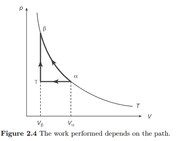
The second law of thermodynamics concerns the nonexistence of a perpetuum mobile. This has long been a contentious issue but it is based on one of the most obvious facts of everyday experience, namely that certain processes are irreversible. This means simply that they cannot be reversed in time. Thus, e.g. the breaking of a glass on the floor is an irreversible process because the reverse process: the spontaneous creation of a glass from pieces on the floor simply does not happen. Characteristic of a process like that is that an ordered structure is destroyed which cannot be recreated without “doing something” to the system. It makes sense, therefore, to postulate the existence of a measure for the order in the system. Traditionally, one has chosen to introduce a measure of disorder instead, which is called the entropy. The second law is then a formulation of the creation of entropy in processes where the system is undisturbed. The first precise formulation of the second law was given by Lord Kelvin and Clausius. Kelvin’s formulation reads as follows.
There exists no thermodynamic transformation of which the only result is to convert heat from a heat reservoir to work.
Clausius’ formulation is slightly different.
There exists no thermodynamic transformation of which the only result is the transfer of heat from a colder heat reservoir to a hotter heat reservoir.
Clausius deduced from these basic statements the existence of a function of state which can only increase if the system is thermally isolated. This is the entropy which we simply postulate to exist. We then show in chapter 5 that our formulation implies their original statements.
To formulate the law in its entirety we need the following observation:
All thermodynamic parameters can be divided into two categories, namely intensive and extensive parameters. Intensive parameters are thermodynamic parameters that are independent of the size of the system; extensive parameters are thermodynamic parameters that are directly proportional to the size of the system.

物理代写|统计力学代写Statistical mechanics代考|Thermal Engines and Refrigerators

Thermodynamics was developed in a study of the efficient operation of thermal engines, the steam engine in particular. It is still important for these applications, e.g. the car engine, refrigerators, and steam turbines in electricity plants. The principle of operation of a heat engine is pictured schematically in figure 5.1.

Heat is absorbed from a heat reservoir at temperature $T_{A}$. The engine $E$ converts part of this heat into useful work $W$ and rejects the surplus heat $Q_{B}$ to a second heat reservoir at temperature $T_{B}$. Clearly,
$$
W=Q_{A}-Q_{B}
$$

The efficiency of the engine is defined as
$$
\eta=\frac{W}{Q_{A}} .
$$
Obviously, $\eta \leqslant 1$, but the second law gives a more stringent bound on the efficiency. Indeed, since
$$
\Delta S=-\frac{Q_{A}}{T_{A}}+\frac{Q_{B}}{T_{B}} \geqslant 0
$$
we find
$$
\eta \leqslant 1-\frac{T_{B}}{T_{A}} \equiv \eta_{C}
$$
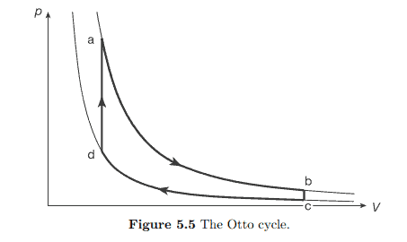
The maximum attainable efficiency $\eta_{C}$ is called the Carnot efficiency. It also follows that the most efficient engines are reversible, $\Delta S=0$. An example of a process in which the Carnot efficiency is attained is the Carnot process. For an ideal gas this process is represented by the cycle abcd in the following $p-V$ diagram of figure $5.2$.

$\mathrm{ab}$ and cd are isotherms, bc and da are adiabatics. In practice this process is very difficult to carry out. Most practical electricity plants use steam as working fluid. The process can then take place inside the coexistence region of steam and liquid water. This is called wet steam. It is then much easier to keep the temperature constant during the transfer of heat as the evaporation occurs at constant temperature. The process is most conveniently represented in a $T-s$ diagram (figure $5.3$ ).

In fact, the actual process used in practical power plants is considerably more complicated. Let us consider two of the most important modifications.

物理代写|统计力学代写Statistical mechanics代考|The Fundamental Equation

In this chapter, we show that the thermodynamics of a (simple) system is completely determined by a single function: the entropy density as a function of the internal energy density and the specific volume. This function has an important property, namely concavity, which enables us to define a number of other thermodynamic functions in chapter 8. Let us recall the definition of convex and concave functions: $A$ region $D$ in $\mathbb{R}^{k}$ is called convex if for every
two points $\vec{x}, \vec{y} \in D$ and every $t \in[0,1]$, also $t \vec{x}+(1-t) \vec{y} \in D$. A function $g: D \rightarrow \mathbb{R} \cup{+\infty}$ from a convex region $D \subset \mathbb{R}^{k}$ to the real line united with $+\infty$ is called convex if, for every $t \in[0,1]$ and all $\vec{x}, \vec{y} \in D$,
$$
g(t \vec{x}+(1-t) \vec{y}) \leqslant \operatorname{tg}(\vec{x})+(1-t) g(\vec{y})
$$
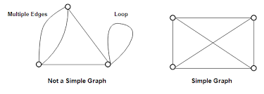
$g$ is called concave if $-g$ is convex. A region $D$ is convex when it does not have dents. Figures $6.1$ (a) and $6.1$ (b) show a convex region and a non-convex region respectively.

Similarly, a function is convex if its graph is everywhere bending upwards. In chapter 7 , we state and prove various useful facts about convex functions. Here, we first outline the significance for thermodynamic functions.

In the introduction and also in chapter 4 we remarked that, in order to describe a macroscopic system mathematically we have to take the thermodynamic limit, i.e. the limit of an infinitely large system with a finite particle number density: $N \rightarrow \infty, V \rightarrow \infty ; \quad \rho=N / V$ fixed. We also write $v=1 / \rho$ for the specific volume. In this limit all surface effects disappear and we are left with the pure bulk properties of the system. For intensive parameters $X(N, V, T)$ we expect the limit
$$
\lim {N, V \rightarrow \infty ; V / N=v} X(N, V, T)=x(v, T) $$ to exist, while for extensive variables $Y(N, V, T)$ we expect the limit $$ \lim {N, V \rightarrow \infty ; V / N=v} \frac{Y(N, V, T)}{N}=y(v, T)
$$
to exist. In other words, $X(N, V, T)=x(v, T)+o(1)$ and $Y(N, V, T)=$ $N y(v, T)+o(N)$ as $N \rightarrow \infty$. In fact, in real systems the values of $X$ and $Y / N$ fluctuate around their mean values $x(v, T)$ and $y(v, T)$.

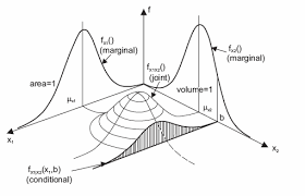
Let us now concentrate in particular on the entropy density for a simple system defined by
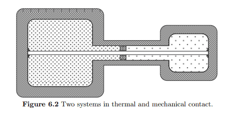
$$
s(u, v)=\lim {N, V \rightarrow \infty ; V / N=v} \frac{1}{N} S(N u, V, N) $$ We shall argue that this function is concave in both its arguments. To show this we consider two systems $\Sigma{1}$ with parameters $\left(U_{1}, V_{1}, N_{1}\right)$ and $\Sigma_{2}$ with parameters $\left(U_{2}, V_{2}, N_{2}\right)$, which are brought into thermal and mechanical contact so that they can exchange energy and their relative volumes ean adjust. Figure $6.2$ gives an impression of this situation.

统计力学代考

物理代写|统计力学代写Statistical mechanics代考|The Second Law

热力学第二定律与永动机的不存在有关。这一直是一个有争议的问题，但它基于日常经验中最明显的事实之一，即某些过程是不可逆的。这意味着它们不能及时逆转。因此，例如在地板上打碎玻璃是一个不可逆的过程，因为相反的过程：从地板上的碎片自发地产生玻璃根本不会发生。像这样的过程的特征是有序结构被破坏，如果不对系统“做某事”就无法重新创建。因此，假设系统中存在秩序度量是有道理的。传统上，人们选择引入一种无序度量，称为熵。然后，第二定律是在系统不受干扰的过程中创建熵的公式。第二定律的第一个精确表述是由开尔文勋爵和克劳修斯给出的。开尔文的公式如下。
不存在唯一的结果是将热量从储热器转换为功的热力学转换。
克劳修斯的表述略有不同。
不存在唯一的结果是将热量从较冷的储热器转移到较热的储热器的热力学转换。
克劳修斯从这些基本陈述中推断出状态函数的存在，该函数只有在系统热隔离时才会增加。这是我们简单假设存在的熵。然后我们在第 5 章中表明，我们的表述暗示了它们的原始陈述。
为了完整地制定法律，我们需要以下观察：
所有的热力学参数都可以分为两类，即密集参数和扩展参数。密集参数是与系统大小无关的热力学参数；扩展参数是与系统大小成正比的热力学参数。

物理代写|统计力学代写Statistical mechanics代考|Thermal Engines and Refrigerators

热力学是在研究热机，特别是蒸汽机的有效运行时发展起来的。对于这些应用，例如汽车发动机、冰箱和发电厂中的蒸汽轮机，它仍然很重要。热机的工作原理如图 5.1 所示。

在一定温度下从储热器中吸收热量吨一个. 引擎和将部分热量转化为有用功在并排出多余的热量问乙到第二个热库在温度吨乙. 清楚地，

在=问一个−问乙

发动机的效率定义为

这=在问一个.
明显地，这⩽1，但第二定律对效率给出了更严格的限制。确实，自从

Δ小号=−问一个吨一个+问乙吨乙⩾0
我们发现

这⩽1−吨乙吨一个≡这C
可达到的最大效率这C称为卡诺效率。最有效的引擎也是可逆的，Δ小号=0. 获得卡诺效率的过程的一个例子是卡诺过程。对于理想气体，这个过程由下面的循环 abcd 表示p−在图形示意图5.2.

一个bcd 是等温线，bc 和 da 是绝热线。在实践中，这个过程很难进行。大多数实际的发电厂使用蒸汽作为工作流体。然后该过程可以在蒸汽和液态水的共存区域内进行。这称为湿蒸汽。由于蒸发发生在恒定温度下，因此在热传递过程中保持温度恒定会容易得多。该过程最方便地表示为吨−s图（图5.3 ).

事实上，实际发电厂中使用的实际过程要复杂得多。让我们考虑两个最重要的修改。

物理代写|统计力学代写Statistical mechanics代考|The Fundamental Equation

在本章中，我们展示了（简单）系统的热力学完全由一个函数决定：熵密度是内能密度和比容的函数。这个函数有一个重要的性质，即凹性，它使我们能够在第 8 章中定义许多其他热力学函数。让我们回顾一下凸函数和凹函数的定义：一个地区D在Rķ被称为凸如果对于每
两个点X→,是→∈D和每一个吨∈[0,1]，还吨X→+(1−吨)是→∈D. 一个函数G:D→R∪+∞从凸区域D⊂Rķ到实线联合+∞称为凸如果，对于每个吨∈[0,1]和所有X→,是→∈D,

G(吨X→+(1−吨)是→)⩽tg⁡(X→)+(1−吨)G(是→)
G称为凹如果−G是凸的。一个地区D没有凹痕时是凸的。数字6.1(a) 和6.1(b) 分别表示凸区域和非凸区域。

类似地，如果函数的图形处处向上弯曲，则该函数是凸函数。在第 7 章中，我们陈述并证明了关于凸函数的各种有用事实。在这里，我们首先概述热力学函数的重要性。

在引言和第 4 章中，我们指出，为了在数学上描述宏观系统，我们必须采用热力学极限，即具有有限粒子数密度的无限大系统的极限：ñ→∞,在→∞;ρ=ñ/在固定的。我们也写在=1/ρ对于特定的音量。在这个极限内，所有的表面效应都消失了，我们只剩下系统的纯体积特性。对于密集参数X(ñ,在,吨)我们期望极限

林ñ,在→∞;在/ñ=在X(ñ,在,吨)=X(在,吨)存在，而对于广泛的变量是(ñ,在,吨)我们期望极限

林ñ,在→∞;在/ñ=在是(ñ,在,吨)ñ=是(在,吨)
存在。换句话说，X(ñ,在,吨)=X(在,吨)+○(1)和是(ñ,在,吨)= ñ是(在,吨)+○(ñ)作为ñ→∞. 事实上，在实际系统中，X和是/ñ围绕它们的平均值波动X(在,吨)和是(在,吨).

现在让我们特别关注由下式定义的简单系统的熵密度

s(在,在)=林ñ,在→∞;在/ñ=在1ñ小号(ñ在,在,ñ)我们将论证这个函数在它的两个参数中都是凹的。为了证明这一点，我们考虑两个系统Σ1带参数(在1,在1,ñ1)和Σ2带参数(在2,在2,ñ2)，它们被带入热和机械接触，以便它们可以交换能量并且它们的相对体积可以调整。数字6.2给人这种情况的印象。

物理代写|统计力学代写Statistical mechanics代考请认准statistics-lab™

统计代写请认准statistics-lab™. statistics-lab™为您的留学生涯保驾护航。

金融工程代写

金融工程是使用数学技术来解决金融问题。金融工程使用计算机科学、统计学、经济学和应用数学领域的工具和知识来解决当前的金融问题，以及设计新的和创新的金融产品。

非参数统计代写

非参数统计指的是一种统计方法，其中不假设数据来自于由少数参数决定的规定模型；这种模型的例子包括正态分布模型和线性回归模型。

广义线性模型代考

广义线性模型（GLM）归属统计学领域，是一种应用灵活的线性回归模型。该模型允许因变量的偏差分布有除了正态分布之外的其它分布。

术语广义线性模型（GLM）通常是指给定连续和/或分类预测因素的连续响应变量的常规线性回归模型。它包括多元线性回归，以及方差分析和方差分析（仅含固定效应）。

有限元方法代写

有限元方法（FEM）是一种流行的方法，用于数值解决工程和数学建模中出现的微分方程。典型的问题领域包括结构分析、传热、流体流动、质量运输和电磁势等传统领域。

有限元是一种通用的数值方法，用于解决两个或三个空间变量的偏微分方程（即一些边界值问题）。为了解决一个问题，有限元将一个大系统细分为更小、更简单的部分，称为有限元。这是通过在空间维度上的特定空间离散化来实现的，它是通过构建对象的网格来实现的：用于求解的数值域，它有有限数量的点。边界值问题的有限元方法表述最终导致一个代数方程组。该方法在域上对未知函数进行逼近。[1] 然后将模拟这些有限元的简单方程组合成一个更大的方程系统，以模拟整个问题。然后，有限元通过变化微积分使相关的误差函数最小化来逼近一个解决方案。

tatistics-lab作为专业的留学生服务机构，多年来已为美国、英国、加拿大、澳洲等留学热门地的学生提供专业的学术服务，包括但不限于Essay代写，Assignment代写，Dissertation代写，Report代写，小组作业代写，Proposal代写，Paper代写，Presentation代写，计算机作业代写，论文修改和润色，网课代做，exam代考等等。写作范围涵盖高中，本科，研究生等海外留学全阶段，辐射金融，经济学，会计学，审计学，管理学等全球99%专业科目。写作团队既有专业英语母语作者，也有海外名校硕博留学生，每位写作老师都拥有过硬的语言能力，专业的学科背景和学术写作经验。我们承诺100%原创，100%专业，100%准时，100%满意。

随机分析代写

随机微积分是数学的一个分支，对随机过程进行操作。它允许为随机过程的积分定义一个关于随机过程的一致的积分理论。这个领域是由日本数学家伊藤清在第二次世界大战期间创建并开始的。

时间序列分析代写

随机过程，是依赖于参数的一组随机变量的全体，参数通常是时间。随机变量是随机现象的数量表现，其时间序列是一组按照时间发生先后顺序进行排列的数据点序列。通常一组时间序列的时间间隔为一恒定值（如1秒，5分钟，12小时，7天，1年），因此时间序列可以作为离散时间数据进行分析处理。研究时间序列数据的意义在于现实中，往往需要研究某个事物其随时间发展变化的规律。这就需要通过研究该事物过去发展的历史记录，以得到其自身发展的规律。

回归分析代写

多元回归分析渐进（Multiple Regression Analysis Asymptotics）属于计量经济学领域，主要是一种数学上的统计分析方法，可以分析复杂情况下各影响因素的数学关系，在自然科学、社会和经济学等多个领域内应用广泛。

MATLAB代写

MATLAB 是一种用于技术计算的高性能语言。它将计算、可视化和编程集成在一个易于使用的环境中，其中问题和解决方案以熟悉的数学符号表示。典型用途包括：数学和计算算法开发建模、仿真和原型制作数据分析、探索和可视化科学和工程图形应用程序开发，包括图形用户界面构建MATLAB 是一个交互式系统，其基本数据元素是一个不需要维度的数组。这使您可以解决许多技术计算问题，尤其是那些具有矩阵和向量公式的问题，而只需用 C 或 Fortran 等标量非交互式语言编写程序所需的时间的一小部分。MATLAB 名称代表矩阵实验室。MATLAB 最初的编写目的是提供对由 LINPACK 和 EISPACK 项目开发的矩阵软件的轻松访问，这两个项目共同代表了矩阵计算软件的最新技术。MATLAB 经过多年的发展，得到了许多用户的投入。在大学环境中，它是数学、工程和科学入门和高级课程的标准教学工具。在工业领域，MATLAB 是高效研究、开发和分析的首选工具。MATLAB 具有一系列称为工具箱的特定于应用程序的解决方案。对于大多数 MATLAB 用户来说非常重要，工具箱允许您学习和应用专业技术。工具箱是 MATLAB 函数（M 文件）的综合集合，可扩展 MATLAB 环境以解决特定类别的问题。可用工具箱的领域包括信号处理、控制系统、神经网络、模糊逻辑、小波、仿真等。

R语言代写	问卷设计与分析代写
PYTHON代写	回归分析与线性模型代写
MATLAB代写	方差分析与试验设计代写
STATA代写	机器学习/统计学习代写
SPSS代写	计量经济学代写
EVIEWS代写	时间序列分析代写
EXCEL代写	深度学习代写
SQL代写	各种数据建模与可视化代写

物理代写|统计力学代写Statistical mechanics代考|PHYS3034

Posted on 2022年6月27日2022年6月27日 by statistics-lab

如果你也在怎样代写统计力学Statistical mechanics这个学科遇到相关的难题，请随时右上角联系我们的24/7代写客服。

我们提供的统计力学Statistical mechanics及其相关学科的代写，服务范围广, 其中包括但不限于:

Statistical Inference 统计推断
Statistical Computing 统计计算
Advanced Probability Theory 高等概率论
Advanced Mathematical Statistics 高等数理统计学
(Generalized) Linear Models 广义线性模型
Statistical Machine Learning 统计机器学习
Longitudinal Data Analysis 纵向数据分析
Foundations of Data Science 数据科学基础

物理代写|统计力学代写Statistical mechanics代考|PHYS3034

物理代写|统计力学代写Statistical mechanics代考|The Zeroth Law

The zeroth law states:
There exists a function of state $T$, the temperature, such that two systems in thermal contact are in thermal equilibrium if and only if their temperatures are equal.
Note that this law does not fix the temperature scale! On the Celsius scale, one defines $0^{\circ} \mathrm{C}$ as the melting point of ice and $100^{\circ} \mathrm{C}$ as the boiling point of water, both under a pressure of $1 \mathrm{~atm}$. The temperature of a given system can then be determined by bringing it into thermal contact with a thermometer and measuring some property of the thermometer system using linear interpolation between $0^{\circ} \mathrm{C}$ and $100^{\circ} \mathrm{C}$ (and extrapolation beyond this range).
EXAMPLE 1.1: Mercury vs. Resistance Thermometer.
In a mercury thermometer for example, the temperature is determined by the length of a column of mercury as it expands due to heating. Thus:
$$
\theta_{m}=\frac{\ell_{\theta}-\ell_{0}}{\ell_{100}-\ell_{0}} \times 100^{\circ} \mathrm{C}
$$
is the empirical temperature as it is measured by a mercury thermometer. In a resistance thermometer, the temperature is determined by the electrical resistance of a metal wire:
$$
\theta_{R}=\frac{R_{\theta}-R_{0}}{R_{100}-R_{0}} \times 100^{\circ} \mathrm{C} .
$$
We now encounter the following problem: Suppose that the electrical resistance $R$ varies nonlinearly with temperature as measured on the mercury scảlé:
$$
R_{\theta}=R_{0}\left(1+b \theta_{m}+c \theta_{m}^{2}\right)
$$
Then
$$
\theta_{R}=\frac{b \theta_{m}+c \theta_{m}^{2}}{b+100 c} \neq \theta_{m}
$$

Fortunately, it turns out that the nonlinearity in equation (1.3) is rather small over a not too large interval of temperatures. (i.e. $c<<1$.) Nevertheless, for an accurate definition of the temperature scale one needs a standard thermometer with which all other thermometers can then be gauged. For this we can use an inert gas. Indeed, using one of the above types of thermometer, it was discovered that most rare gases satisfy the ideal gas law (1) mentioned in the introduction:
$$
p V=n R_{0} T,
$$
where the constant $R_{0}$ is independent of the gas and where $T=\theta+273$ if $\theta$ is measured in degrees Celsius.

物理代写|统计力学代写Statistical mechanics代考|The First Law

The first law of thermodynamics is an extension of the law of conservation of energy to include thermal processes. It can be formulated as follows:
There exists a function of state $U$, the internal energy, such that if an amount of energy $E$ is supplied to an otherwise isolated system, bringing it from an equilibrium state $\alpha$ to an equilibrium state $\beta$, then
$$
E=U(\beta)-U(\alpha)
$$
irrespective of the way in which this energy was supplied.

EXAMPLE 2.1: The sledge.
Consider a sledge of mass $M$ sliding down a hill of height $h$ (figure 2.1). Assume that the speed of the sledge at the top of the hill is negligible. By conservation of energy, the potential energy $E_{p o t}=M g h$ must have been transformed into kinetic energy: $E_{k i n}=\frac{1}{2} M v^{2}$ at the bottom of the hill. The speed at the bottom of the hill must be $v=\sqrt{2 g h}$. In fact the speed will be smaller due to friction. Where has the energy gone? The answer is, of course, that it was transformed into heat.

The first precise experiments about heat flow were done by James Joule in the $1840 \mathrm{~s}$. He did measurements on a thermally insulated container of gas to which he supplied energy in different ways: mechanical stirring, electrical heating, and compression. Figure $2.2$ shows the three processes schematically. Joule found that the final temperature of the gas depends only on the amount of energy supplied; not on the way it was supplied, whether it was heat or work. Note that it was important that the container was well-insulated so that no heat could escape. In that case all the energy supplied must have been absorbed by the gas. In each of the different ways of heating the gas, it is possible to determine the amount of energy supplied, and it turns out that this determines the final state of the gas completely.

物理代写|统计力学代写Statistical mechanics代考|Differentials

In this chapter we derive some c

onsequences of the first law. The first law is used most often in differential form. This is particularly useful for quasi-static processes, which can be subdivided into small stages during which the change in the various state functions is only small (infinitesimal). In infinitesimal form, the equation (2.10) reads:
$$
\delta Q+\delta W=\mathrm{d} U
$$
One can give a precise meaning to the differential quantities appearing in this equation by defining the concept of a differential form. We shall discuss this at the end of this chapter, but first let us do some formal calculations with the differential forms appearing in (3.1).

In example $2.2$ we already mentioned that the work differential $\delta W$ cannot be written as a small change in a function of state $\mathcal{W}$. We shall use the notation $\delta$ in such a case. On the other hand, the differential $\mathrm{d} U$ does mean: ‘a small change in $U^{\prime}$, and we write $\mathrm{d}$ instead of $\delta$. One says that the differential $\mathrm{d} U$ is exact. If we assume as basic coordinates of the state space $V$ and $T$ we can write $\mathrm{d} U$ in terms of the coordinate differentials $\mathrm{d} V$ and $\mathrm{d} T$ :
$$
\mathrm{d} U=\left(\frac{\partial U}{\partial T}\right){V} \mathrm{~d} T+\left(\frac{\partial U}{\partial V}\right){T} \mathrm{~d} V=C_{V} \mathrm{~d} T+\left(\frac{\partial U}{\partial V}\right){T} \mathrm{~d} V $$ (The subscript on partial derivatives indicates the variable to be kept fixed.) We have already seen that the work differential can also be written in terms of $\mathrm{d} T$ and $\mathrm{d} V$ (in fact only the latter appears): $$ \delta W=-p \mathrm{~d} V . $$ In general, one can write any arbitrary differential in terms of the coordinate differentials. Denoting an arbitrary differential by $\omega$, one has $$ \omega=f{1}(T, V) \mathrm{d} T+f_{2}(T, V) \mathrm{d} V
$$

Using equation (3.1) we have for the heat differential
$$
\delta Q=C_{V} \mathrm{~d} T+\left(p+\left(\frac{\partial U}{\partial V}\right){T}\right) \mathrm{d} V $$ Alternatively, one can take $T$ and $p$ as independent variables and write $$ \mathrm{d} U=\left(\frac{\partial U}{\partial T}\right){p} \mathrm{~d} T+\left(\frac{\partial U}{\partial p}\right)_{T} \mathrm{~d} p
$$

统计力学代考

物理代写|统计力学代写Statistical mechanics代考|The Zeroth Law

第零定律指出：
存在状态的函数吨，温度，使得两个热接触系统处于热平衡当且仅当它们的温度相等时。
请注意，该定律不固定温标！在摄氏温度范围内，一个定义0∘C作为冰的熔点和100∘C作为水的沸点，在压力下1 一个吨米. 然后可以通过将给定系统与温度计热接触并使用之间的线性插值测量温度计系统的某些属性来确定给定系统的温度0∘C和100∘C（以及超出此范围的外推）。
例 1.1：水银与电阻温度计。
例如，在水银温度计中，温度由水银柱的长度决定，因为水银柱因受热而膨胀。因此：

θ米=ℓθ−ℓ0ℓ100−ℓ0×100∘C
是通过水银温度计测量的经验温度。在电阻温度计中，温度由金属线的电阻决定：

θR=Rθ−R0R100−R0×100∘C.
我们现在遇到以下问题：假设电阻R在水银镜上测量的温度随温度非线性变化：

Rθ=R0(1+bθ米+Cθ米2)
然后

θR=bθ米+Cθ米2b+100C≠θ米

幸运的是，方程 (1.3) 中的非线性在不太大的温度区间内相当小。（IEC<<1.) 然而，为了准确定义温标，需要一个标准温度计，然后可以测量所有其他温度计。为此，我们可以使用惰性气体。事实上，使用上述类型的温度计之一，发现大多数稀有气体满足引言中提到的理想气体定律（1）：

p在=nR0吨,
其中常数R0与气体无关，在哪里吨=θ+273如果θ以摄氏度为单位测量。

物理代写|统计力学代写Statistical mechanics代考|The First Law

热力学第一定律是能量守恒定律的延伸，包括热过程。可以表述为：
存在状态函数在, 内能, 这样如果一定量的能量和提供给一个原本孤立的系统，使其脱离平衡状态一个达到平衡状态b，然后

和=在(b)−在(一个)
无论这种能量的供应方式如何。

例 2.1：雪橇。
考虑一个质量雪橇米从高处滑下H（图 2.1）。假设山顶雪橇的速度可以忽略不计。通过能量守恒，势能和p○吨=米GH一定已经转化为动能：和ķ一世n=12米在2在山脚下。山脚下的速度必须是在=2GH. 事实上，由于摩擦，速度会变小。能量去哪儿了？答案当然是它转化为热量。

关于热流的第一个精确实验是由 James Joule 在1840 s. 他在一个隔热的气体容器上进行了测量，他以不同的方式向该容器提供能量：机械搅拌、电加热和压缩。数字2.2示意性地显示了这三个过程。焦耳发现气体的最终温度仅取决于所提供的能量数量；不是在供应的方式上，无论是热量还是工作。请注意，重要的是容器绝缘良好，以免热量逸出。在这种情况下，所提供的所有能量都必须被气体吸收。在加热气体的每一种不同方式中，都可以确定提供的能量量，事实证明，这完全决定了气体的最终状态。

物理代写|统计力学代写Statistical mechanics代考|Differentials

在本章中，我们推导出一些 c

第一定律的后果。第一定律最常以微分形式使用。这对于准静态过程特别有用，准静态过程可以细分为小阶段，在这些阶段中，各种状态函数的变化很小（无穷小）。以无穷小的形式，等式 (2.10) 为：

d问+d在=d在
通过定义微分形式的概念，可以给这个方程中出现的微分量一个精确的含义。我们将在本章末尾讨论这个问题，但首先让我们用 (3.1) 中出现的微分形式做一些正式的计算。

在示例中2.2我们已经提到工作差异d在不能写成状态函数的微小变化在. 我们将使用符号d在这种情况下。另一方面，微分d在确实意味着：’一个小的变化在′，我们写d代替d. 有人说差速器d在是准确的。如果我们假设状态空间的基本坐标在和吨我们可以写d在就坐标微分而言d在和d吨 :

d在=(∂在∂吨)在 d吨+(∂在∂在)吨 d在=C在 d吨+(∂在∂在)吨 d在（偏导数上的下标表示要保持固定的变量。）我们已经看到，功微分也可以写成d吨和d在（实际上只有后者出现）：

d在=−p d在.一般来说，可以根据坐标微分写出任意微分。表示任意微分ω, 一个有

ω=F1(吨,在)d吨+F2(吨,在)d在

使用方程（3.1），我们得到了热差

d问=C在 d吨+(p+(∂在∂在)吨)d在或者，可以采取吨和p作为自变量并写

d在=(∂在∂吨)p d吨+(∂在∂p)吨 dp

统计代写请认准statistics-lab™. statistics-lab™为您的留学生涯保驾护航。

金融工程代写

非参数统计代写

非参数统计指的是一种统计方法，其中不假设数据来自于由少数参数决定的规定模型；这种模型的例子包括正态分布模型和线性回归模型。

广义线性模型代考

广义线性模型（GLM）归属统计学领域，是一种应用灵活的线性回归模型。该模型允许因变量的偏差分布有除了正态分布之外的其它分布。

有限元方法代写

随机分析代写

时间序列分析代写

回归分析代写

MATLAB代写

R语言代写	问卷设计与分析代写
PYTHON代写	回归分析与线性模型代写
MATLAB代写	方差分析与试验设计代写
STATA代写	机器学习/统计学习代写
SPSS代写	计量经济学代写
EVIEWS代写	时间序列分析代写
EXCEL代写	深度学习代写
SQL代写	各种数据建模与可视化代写

物理代写|统计力学代写Statistical mechanics代考|PHYC90010

Posted on 2022年6月14日2022年6月14日 by statistics-lab

如果你也在怎样代写统计力学Statistical mechanics这个学科遇到相关的难题，请随时右上角联系我们的24/7代写客服。

我们提供的统计力学Statistical mechanics及其相关学科的代写，服务范围广, 其中包括但不限于:

Statistical Inference 统计推断
Statistical Computing 统计计算
Advanced Probability Theory 高等概率论
Advanced Mathematical Statistics 高等数理统计学
(Generalized) Linear Models 广义线性模型
Statistical Machine Learning 统计机器学习
Longitudinal Data Analysis 纵向数据分析
Foundations of Data Science 数据科学基础

物理代写|统计力学代写Statistical mechanics代考|PHYC90010

物理代写|统计力学代写Statistical mechanics代考|Poincaré’s Recurrence Theorem, or The Eternal Return

In words, Poincaré’s recurrence theorem says that, for any measure preserving transformation, almost every trajectory comes back arbitrarily close to its initial condition and does that infinitely often.
That property is called recurrence.
Since we know that the Hamiltonian flow on a constant energy surface preserves the Liouville measure on that surface, it follows that, for any mechanical system bounded (in phase space) almost all configurations will come back infinitely often to a configuration arbitrarily close to itself, or to any other configuration that it visits (since one could always define that configuration as an initial condition).

Thus, bounded mechanical systems do not necessarily have only periodic trajectories but almost all their trajectories have a property somewhat similar but weaker than periodicity, namely recurrence.

If one replaced the measure preserving transformation by a deterministic transformation on a finite set, then, obviously, all trajectories must eventually be periodic

since some element of the finite set must be visited twice (over an infinite time) and from then on, the trajectory becomes periodic.

The genius of Poincaré was to extend this result to a weaker notion (recurrence) for measure preserving transformations on infinite sets but bounded in the sense that the measure of the space on which the transformation acts is finite:

Theorem $4.2$ (Poincaré’s recurrence theorem [261]) Let $(\Omega, \Sigma, \mu)$ be a measure space with $\mu(\Omega)<\infty$, where $\mu$ is $T$-imvariant for $T: \Omega \rightarrow \Omega$. Then, $\forall A \in \Sigma$, with $\mu(A)>0, \exists B \subset A$ with $\mu(A \backslash B)=0$ and such that $\forall x \in B, \exists$ sequence $\left(n_{i}\right){i=1}^{\infty}$, $n{i} \in \mathbb{N}$, with $n_{1}<n_{2}<n_{3} \ldots$ and $T^{n_{i}} x \in A$.

物理代写|统计力学代写Statistical mechanics代考|Proof of Poincaré’s Recurrence Theorem

Let, for $N \geq 0 \quad A_{N}=\bigcup_{n=N} T^{-n} A$. Elements of $A_{N}$ are those that are sent into $A$ by the map $T^{n}$ for some $n \geq N$. Thus, $B=A \cap\left(\bigcap_{N=0}^{\infty} A_{N}\right)$ are the elements of $A$ that come back to $A$ infinitely often, namely that are such that $\forall x \in B$, there exist a

sequence $\left(n_{i}\right)$ as in the theorem: since, for each $x \in B$, there exist arbitrarily large $n^{\prime} s$ with $T^{n} x \in A$, one may construct the sequence inductively by taking $n_{i+1}$ to be the first integer $n$ with $T^{n} x \in A$ strictly larger than $n_{i}$.

Let us show that $\mu(B)=\mu(A)$, which, since $\mu(\Omega)<\infty$, is equivalent to $\mu(A \backslash B)$ $=0\left(\right.$ write $\mu(A)=\mu(B)+\mu(A \backslash B)$ ). One has $T^{-1} A_{N}=A_{N+1}$ and thus $\mu\left(A_{N}\right)=$ $\mu\left(A_{N+1}\right)$, since $\mu$ is $T$-invariant. So, $\mu\left(A_{0}\right)=\mu\left(A_{N}\right), \forall N$. Since $A_{0} \supset A_{1} \supset$ $\ldots \supset A_{N}$, and since $\mu(\Omega)<\infty$, one has $\mu\left(A_{N}\right) \leq \mu\left(A_{0}\right) \leq \mu(\Omega)<\infty$ and thus $\mu\left(A_{0} \backslash A_{N}\right)=\mu\left(A_{0}\right)-\mu\left(A_{N}\right)=0, \forall N$. Since a countable union of sets of measure zero is of measure zero $\mu\left(A_{0} \backslash\left(\bigcap_{N=0}^{\infty} A_{N}\right)\right)=\mu\left(\bigcup_{N=0}^{\infty}\left(A_{0} \backslash A_{N}\right)\right)=0$. Thus, since $\bigcap_{N=0}^{\infty} A_{N} \subset A_{0}, \mu(B)=\mu\left(A \cap\left(\bigcap_{N=0}^{\infty} A_{N}\right)\right)=\mu\left(A \cap A_{0}\right)$ and $\mu\left(A \cap A_{0}\right)=$ $\mu(A)$, since $A \subset A 0$. So, $\mu(B)=\mu(A)$.

物理代写|统计力学代写Statistical mechanics代考|Ergodic Theorems

Although we have not yet defined what unpredictable dynamical systems are, we said that, when a dynamical system is unpredictable, one should study its trajectories by statistical methods. A first step in that direction is to study certain time averages of trajectories, for example the average time spent by the trajectory in a set $A \in \Sigma$. We will study a slightly more general object.

Given a measure space $(\Omega, \Sigma, \mu)$, a map $T: \Omega \rightarrow \Omega$ such that $\mu$ is $T$-invariant, and a $\mu$-integrable function $F: \Omega \rightarrow \mathbb{R}$, one may consider the temporal averages:
$$
\frac{1}{N} \sum_{n=0}^{N-1} F\left(T^{n} x\right)
$$
and ask whether the limits $N \rightarrow \infty$ of those quantities exist.
If one takes $F=\mathbb{1}{A}$, the indicator function of a set $A \in \Sigma$, formula (4.3.1) gives the average time, up to time $N$, spent by the system in $A$, and the limit $N \rightarrow \infty$, if it exists, gives the average time $\tau{A}$ spent in $A$.

The following theorem, that we will not prove because the proof is a bit long and not particularly illuminating (see Walters [327, Sect. 1.6] or Cornfeld, Fomin and Sinai [87, Appendix 3]) asserts that all these limits actually exist ${ }^{4}$ :

统计力学代考

物理代写|统计力学代写Statistical mechanics代考|Poincaré’s Recurrence Theorem, or The Eternal Return

换句话说，庞加莱的递归定理说，对于任何保持测度的变换，几乎每条轨迹都会任意返回到其初始条件，并且会无限频繁地这样做。
该属性称为重复。
由于我们知道恒定能量表面上的哈密顿流保留了该表面上的刘维尔测量，因此，对于任何有界（在相空间中）的机械系统，几乎所有配置都会无限频繁地返回到任意接近自身的配置，或它访问的任何其他配置（因为总是可以将该配置定义为初始条件）。

因此，有界机械系统不一定只有周期性轨迹，但几乎所有的轨迹都具有与周期性有些相似但弱于周期性的性质，即递归。

如果用有限集上的确定性变换代替测度保持变换，那么显然，所有轨迹最终都必须是周期性的

由于必须访问有限集中的某些元素（在无限时间内），从那时起，轨迹就变成了周期性的。

Poincaré 的天才是将这个结果扩展到一个较弱的概念（递归），用于在无限集上保留测度变换，但在变换作用于的空间的测度是有限的意义上是有界的：

定理4.2（Poincaré 的递归定理 [261]）让(Ω,Σ,μ)是一个测度空间μ(Ω)<∞，在哪里μ是吨-不变的吨:Ω→Ω. 然后，∀一个∈Σ，和μ(一个)>0,∃乙⊂一个和μ(一个∖乙)=0并且这样∀X∈乙,∃序列(n一世)一世=1∞, n一世∈ñ，和n1<n2<n3…和吨n一世X∈一个.

物理代写|统计力学代写Statistical mechanics代考|Proof of Poincaré’s Recurrence Theorem

让，对于ñ≥0一个ñ=⋃n=ñ吨−n一个. 要点一个ñ是那些被发送到一个按地图吨n对于一些n≥ñ. 因此，乙=一个∩(⋂ñ=0∞一个ñ)是的元素一个回到一个无限地经常，即是这样的∀X∈乙, 存在一个

序列(n一世)如定理所示：因为，对于每个X∈乙, 存在任意大n′s和吨nX∈一个, 可以通过采取归纳构造序列n一世+1成为第一个整数n和吨nX∈一个严格大于n一世.

让我们证明μ(乙)=μ(一个), 其中, 因为μ(Ω)<∞, 等价于μ(一个∖乙) =0(写μ(一个)=μ(乙)+μ(一个∖乙)）。一个有吨−1一个ñ=一个ñ+1因此μ(一个ñ)= μ(一个ñ+1)，自从μ是吨-不变的。所以，μ(一个0)=μ(一个ñ),∀ñ. 自从一个0⊃一个1⊃ …⊃一个ñ，并且由于μ(Ω)<∞, 一个有μ(一个ñ)≤μ(一个0)≤μ(Ω)<∞因此μ(一个0∖一个ñ)=μ(一个0)−μ(一个ñ)=0,∀ñ. 由于零测度集的可数并集是零测度μ(一个0∖(⋂ñ=0∞一个ñ))=μ(⋃ñ=0∞(一个0∖一个ñ))=0. 因此，由于⋂ñ=0∞一个ñ⊂一个0,μ(乙)=μ(一个∩(⋂ñ=0∞一个ñ))=μ(一个∩一个0)和μ(一个∩一个0)= μ(一个)，自从一个⊂一个0. 所以，μ(乙)=μ(一个).

物理代写|统计力学代写Statistical mechanics代考|Ergodic Theorems

虽然我们还没有定义什么是不可预测的动力系统，但我们说过，当一个动力系统是不可预测的时，应该用统计方法研究它的轨迹。朝着这个方向迈出的第一步是研究轨迹的某些时间平均值，例如一组轨迹所花费的平均时间一个∈Σ. 我们将研究一个稍微更一般的对象。

给定一个测度空间(Ω,Σ,μ)，一张地图吨:Ω→Ω这样μ是吨-不变量，和μ- 可积函数F:Ω→R，可以考虑时间平均值：

1ñ∑n=0ñ−1F(吨nX)
并询问是否限制ñ→∞这些数量存在。
如果一个采取F=1一个, 集合的指示函数一个∈Σ, 公式 (4.3.1) 给出了平均时间, 最多时间ñ, 系统花费在一个, 和极限ñ→∞，如果存在，给出平均时间τ一个花费在一个.

以下定理，我们不会证明，因为证明有点长而且不是特别有启发性（参见 Walters [327，Sect. 1.6] 或 Cornfeld、Fomin 和 Sinai [87，附录 3]）断言所有这些限制确实存在4 :

统计代写请认准statistics-lab™. statistics-lab™为您的留学生涯保驾护航。

金融工程代写

非参数统计代写

非参数统计指的是一种统计方法，其中不假设数据来自于由少数参数决定的规定模型；这种模型的例子包括正态分布模型和线性回归模型。

广义线性模型代考

广义线性模型（GLM）归属统计学领域，是一种应用灵活的线性回归模型。该模型允许因变量的偏差分布有除了正态分布之外的其它分布。

有限元方法代写

随机分析代写

时间序列分析代写

回归分析代写

MATLAB代写

R语言代写	问卷设计与分析代写
PYTHON代写	回归分析与线性模型代写
MATLAB代写	方差分析与试验设计代写
STATA代写	机器学习/统计学习代写
SPSS代写	计量经济学代写
EVIEWS代写	时间序列分析代写
EXCEL代写	深度学习代写
SQL代写	各种数据建模与可视化代写

物理代写|统计力学代写Statistical mechanics代考|PHYC30017

Posted on 2022年6月14日2022年6月14日 by statistics-lab

如果你也在怎样代写统计力学Statistical mechanics这个学科遇到相关的难题，请随时右上角联系我们的24/7代写客服。

我们提供的统计力学Statistical mechanics及其相关学科的代写，服务范围广, 其中包括但不限于:

Statistical Inference 统计推断
Statistical Computing 统计计算
Advanced Probability Theory 高等概率论
Advanced Mathematical Statistics 高等数理统计学
(Generalized) Linear Models 广义线性模型
Statistical Machine Learning 统计机器学习
Longitudinal Data Analysis 纵向数据分析
Foundations of Data Science 数据科学基础

物理代写|统计力学代写Statistical mechanics代考|PHYC30017

物理代写|统计力学代写Statistical mechanics代考|Hamilton’s Equations

It is often convenient to rewrite Newton’s equations (3.2.6) in Lagrangian form or in Hamiltonian form. We will only use the latter one. 4 To do so, we will introduce the phase space $\mathbb{R}^{6 N}$, and write a vector $\mathbf{x} \in \mathbb{R}^{6 \mathbf{N}}$ as a pair $\mathbf{x}=(\mathbf{q}, \mathbf{p})$, with $\mathbf{q}=$ $\left(\vec{q}{1}, \vec{q}{2}, \ldots, \vec{q}{N}\right) \in \mathbb{R}^{3 N}, \mathbf{p}=\left(\vec{p}{1}, \vec{p}{2}, \ldots, \vec{p}{N}\right) \in \mathbb{R}^{3 N}$
The Hamiltonian is a function $H: \mathbb{R}^{6 N} \rightarrow \mathbb{R}:$
$$
H(\mathbf{q}, \mathbf{p})=K(\mathbf{p})+V(\mathbf{q})
$$
with a kinetic energy
$$
K(\mathbf{p})=\sum_{i=1}^{N} \frac{\left|\vec{p}{i}\right|^{2}}{2 m{i}}
$$
and a potential energy $V(\mathbf{q})$ given by (3.2.5).
Then Hamilton’s equations are given by the following pair:
$$
\frac{d \vec{q}{i}(t)}{d t}=\nabla{\bar{p}{i}} H(\mathbf{q}(t), \mathbf{p}(t)) $$ and $$ \frac{d \vec{p}{i}(t)}{d t}=-\nabla_{\bar{q}{i}} H(\mathbf{q}(t), \mathbf{p}(t)), $$ for $i=1, \ldots, N$ With $H$ defined by (3.3.1), (3.3.2), these equations are: $$ \frac{d \vec{q}{i}(t)}{d t}=\frac{\vec{p}{i}(t)}{m{i}}
$$
and
$$
\begin{aligned}
&\frac{d \vec{p}{i}(t)}{d t}=-\nabla{\overline{q_{i}}} V(\mathbf{q}(t)) . \
&x(t)=\frac{x(0)}{1-t x(0)},
\end{aligned}
$$

物理代写|统计力学代写Statistical mechanics代考|The Hamiltonian Flow

Since (3.2.6) and (3.3.5), (3.3.6) are equivalent, if we assume that the potentials are such that a unique solution $\mathbf{q}(t)$ of (3.2.6) exist for all times, we also have, for the pair of (3.3.5), (3.3.6), for any $t_{0} \in \mathbb{R}$ and any initial conditions ( $\mathbf{q}{0}, \mathbf{p}{0}$ ), a unique solution $(\mathbf{q}(t), \mathbf{p}(t))$ satisfying (3.3.5), (3.3.6) for all times and such that $\left(\mathbf{q}\left(t_{0}\right), \mathbf{p}\left(t_{0}\right)\right)=\left(\mathbf{q}{0}, \mathbf{p}{0}\right)$.

It will be convenient to associate to such solutions a family of maps $T^{t}: \mathbb{R}^{6 N} \rightarrow$ $\mathbb{R}^{6 N}$, for $t \in \mathbb{R}$, defined by:
$$
T^{t}(\mathbf{q}, \mathbf{p})=(\mathbf{q}(t), \mathbf{p}(t))
$$

where $(\mathbf{q}(t), \mathbf{p}(t))$ is the unique solution of $(3.3 .5),(3.3 .6)$ satisfying $(\mathbf{q}(0), \mathbf{p}(0))=$ $(\mathbf{q}, \mathbf{p})$

So, the map $T^{t}$ associates to every pair $(\mathbf{q}, \mathbf{p}) \in \mathbb{R}^{6 N}$ the value at time $t$ of the unique solution $(\mathbf{q}(t), \mathbf{p}(t))$ of $(3.3 .5),(3.3 .6)$ that “passes” through the point (q, p) at time 0 . Since the solutions are assumed to exist for all $t \in \mathbb{R}, T^{t}$ is invertible: $T^{t} T^{-t}=$ Id, where Id is the identity operator.
The family of maps $\left(T^{t}\right)_{t \in \mathbb{R}}$ is called the Hamiltonian flow.

物理代写|统计力学代写Statistical mechanics代考|Conservation of Energy

The energy of a mechanical system of the type considered here is a function $E$ : $\mathbb{R}^{6 N} \rightarrow \mathbb{R}$ defined by
$$
E(\mathbf{q}, \mathbf{p})=K(\mathbf{p})+V(\mathbf{q})
$$
with the kinetic energy $K$ (p) defined in (3.3.2) and the potential energy $\mathrm{V}(\mathbf{q})$ defined in (3.2.5). This is of course identical to the Hamiltonian function and the energy, like the potential, is defined up to an additive constant. We have:

Theorem $3.1$ (Conservation of energy) Let $(\mathbf{q}(t), \mathbf{p}(t)$ ) be a solution of (3.3.5), (3.3.6). Then, $\forall t \in \mathbb{R}$ :
$$
\frac{d E(t)}{d t}=0
$$
where $E(t)=E(\mathbf{q}(t), \mathbf{p}(t))$
Proof It is enough to compute the time derivative of $E(t)$, using (3.3.7), (3.3.1), $(3.3 .2)$ :
$$
\frac{d E(\mathbf{q}(t), \mathbf{p}(t))}{d t}=\sum_{i=1}^{N} \frac{\vec{p}{i} \cdot \frac{d \vec{p}{i}(t)}{d t}}{m_{i}}+\sum_{i=1}^{N} \nabla_{\bar{q}{i}} V(\mathbf{q}(t)) \cdot \frac{d \vec{q}{i}(t)}{d t}
$$
By (3.3.5), (3.3.6), this equals 0 .
Remark 3.2 One may rewrite the energy in a more familiar form, using $\vec{p}{i}(t)=$ $\frac{1}{m{i}} \frac{d \vec{a}{u}(t)}{d t}:$ $$ E(t)=\sum{i=1}^{N} \frac{m_{i}\left|\vec{v}{i}(t)\right|^{2}}{2}+V(\mathbf{q}(t)) $$ with $\vec{v}{i}(t)=\frac{d \vec{q}_{.}(t)}{d t}$.

统计力学代考

物理代写|统计力学代写Statistical mechanics代考|Hamilton’s Equations

用拉格朗日形式或哈密顿形式重写牛顿方程 (3.2.6) 通常很方便。我们只会使用后一种。4 为此，我们将引入相空间R6ñ, 并写一个向量X∈R6ñ作为一对X=(q,p)，和q= (q→1,q→2,…,q→ñ)∈R3ñ,p=(p→1,p→2,…,p→ñ)∈R3ñ
哈密顿量是一个函数H:R6ñ→R:

H(q,p)=ķ(p)+在(q)
具有动能

ķ(p)=∑一世=1ñ|p→一世|22米一世
和势能在(q)由（3.2.5）给出。
然后 Hamilton 方程由以下对给出：

dq→一世(吨)d吨=∇p¯一世H(q(吨),p(吨))和

dp→一世(吨)d吨=−∇q¯一世H(q(吨),p(吨)),为了一世=1,…,ñ和H由 (3.3.1), (3.3.2) 定义，这些方程是：

dq→一世(吨)d吨=p→一世(吨)米一世
和

dp→一世(吨)d吨=−∇q一世¯在(q(吨)). X(吨)=X(0)1−吨X(0),

物理代写|统计力学代写Statistical mechanics代考|The Hamiltonian Flow

由于 (3.2.6) 和 (3.3.5), (3.3.6) 是等价的，如果我们假设势能是唯一解q(吨)的 (3.2.6) 永远存在，我们也有，对于 (3.3.5) 的对， (3.3.6)，对于任何吨0∈R和任何初始条件（q0,p0)，一个独特的解决方案(q(吨),p(吨))始终满足 (3.3.5), (3.3.6) 并且使得(q(吨0),p(吨0))=(q0,p0).

将一系列地图与此类解决方案相关联会很方便吨吨:R6ñ→ R6ñ，为了吨∈R，被定义为：

吨吨(q,p)=(q(吨),p(吨))

在哪里(q(吨),p(吨))是的唯一解(3.3.5),(3.3.6)令人满意的(q(0),p(0))= (q,p)

所以，地图吨吨关联到每一对(q,p)∈R6ñ当时的价值吨的唯一解决方案(q(吨),p(吨))的(3.3.5),(3.3.6)在时间 0 “通过”点 (q, p)。由于假设解决方案对所有人都存在吨∈R,吨吨是可逆的：吨吨吨−吨=Id，其中 Id 是身份运算符。
地图家族(吨吨)吨∈R称为哈密顿流。

物理代写|统计力学代写Statistical mechanics代考|Conservation of Energy

此处考虑的类型的机械系统的能量是一个函数和 : R6ñ→R被定义为

和(q,p)=ķ(p)+在(q)
与动能ķ(p) 在 (3.3.2) 中定义和势能在(q)在 (3.2.5) 中定义。这当然与哈密顿函数相同，并且能量，就像势能一样，被定义为一个加法常数。我们有：

定理3.1（能量守恒）让(q(吨),p(吨)) 是 (3.3.5), (3.3.6) 的解。然后，∀吨∈R :

d和(吨)d吨=0
在哪里和(吨)=和(q(吨),p(吨))
证明计算时间导数就足够了和(吨), 使用 (3.3.7), (3.3.1),(3.3.2):

d和(q(吨),p(吨))d吨=∑一世=1ñp→一世⋅dp→一世(吨)d吨米一世+∑一世=1ñ∇q¯一世在(q(吨))⋅dq→一世(吨)d吨
通过 (3.3.5), (3.3.6)，这等于 0 。
备注 3.2 可以用更熟悉的形式重写能量，使用p→一世(吨)= 1米一世d一个→在(吨)d吨:

和(吨)=∑一世=1ñ米一世|在→一世(吨)|22+在(q(吨))和在→一世(吨)=dq→.(吨)d吨.

统计代写请认准statistics-lab™. statistics-lab™为您的留学生涯保驾护航。

金融工程代写

非参数统计代写

非参数统计指的是一种统计方法，其中不假设数据来自于由少数参数决定的规定模型；这种模型的例子包括正态分布模型和线性回归模型。

广义线性模型代考

广义线性模型（GLM）归属统计学领域，是一种应用灵活的线性回归模型。该模型允许因变量的偏差分布有除了正态分布之外的其它分布。

有限元方法代写

随机分析代写

时间序列分析代写

回归分析代写

MATLAB代写

R语言代写	问卷设计与分析代写
PYTHON代写	回归分析与线性模型代写
MATLAB代写	方差分析与试验设计代写
STATA代写	机器学习/统计学习代写
SPSS代写	计量经济学代写
EVIEWS代写	时间序列分析代写
EXCEL代写	深度学习代写
SQL代写	各种数据建模与可视化代写

物理代写|统计力学代写Statistical mechanics代考|PHYS3006

Posted on 2022年6月14日2022年6月14日 by statistics-lab

如果你也在怎样代写统计力学Statistical mechanics这个学科遇到相关的难题，请随时右上角联系我们的24/7代写客服。

我们提供的统计力学Statistical mechanics及其相关学科的代写，服务范围广, 其中包括但不限于:

Statistical Inference 统计推断
Statistical Computing 统计计算
Advanced Probability Theory 高等概率论
Advanced Mathematical Statistics 高等数理统计学
(Generalized) Linear Models 广义线性模型
Statistical Machine Learning 统计机器学习
Longitudinal Data Analysis 纵向数据分析
Foundations of Data Science 数据科学基础

物理代写|统计力学代写Statistical mechanics代考|PHYS3006

物理代写|统计力学代写Statistical mechanics代考|Cantor Sets and Measures

As an aside, we mention a family of sets that are interesting from a topological and measure-theoretic viewpoint: the Cantor sets.

The original or “middle-third” Cantor set can be obtained by removing successively the “middle-third” intervals: let $C_{0}=[0,1], C_{1}=[0,1] \backslash(] \frac{1}{3}, \frac{2}{3}[)=\left[0, \frac{1}{3}\right] \cup$ $\left[\frac{1}{3}, 1\right], \quad C_{2}=C_{1} \backslash(] \frac{1}{9}, \frac{2}{9}[\cup] \frac{7}{9}, \frac{8}{9}[)=\left[0, \frac{1}{9}\right] \cup\left[\frac{2}{9}, \frac{1}{3}\right] \cup\left[\frac{2}{3}, \frac{7}{9}\right] \cup\left[\frac{8}{9}, 1\right]$, and so on. Then $C=n_{n=0}^{\infty} C_{n}$.

Actually, $C=\left{x \mid x=\sum_{n=1}^{\infty} \frac{a_{n}}{3^{n}}, a_{n} \neq 1, \forall n\right}$. To see this, observe that, if we write the ternary expansion of a number $x \in[0,1], x=\sum_{n=1}^{\infty} \frac{a_{n}}{3 \pi}$, then the numbers in $] \frac{1}{3}, \frac{2}{3}\left[\right.$ correspond to $a_{1}=1$ those in $] \frac{1}{9}, \frac{2}{9}[\cup] \frac{7}{9}, \frac{8}{9}\left[\right.$ correspond to $a_{2}=1$ and so on. So that the numbers in $C$ are exactly those $x \in[0,1]$ whose ternary expansion does not contain the symbol 1 .
The Cantor set $C$ has the following properties:

$C$ is of zero measure since the sum of the lengths of the removed intervals is: $\sum_{n=1}^{\infty} \frac{2^{n-1}}{3 n}=1$.
$C$ is uncountable: the map $g: C \rightarrow[0,1], \quad g(x)=\sum_{n=1}^{\infty} \frac{a_{n}}{2^{n+1}}$, where $x=\sum_{n=1}^{\infty} \frac{a_{n}}{3 n}, a_{n} \neq 1, \forall n$, is a surjection from $C$ to $[0,1]$, hence the cardinality of $C$ must be at least the one of $[0,1]$ (and also at most that cardinality, since $C \subset[0,1])$.
$C$ is a perfect set, which, by definition, means that it is closed (since it is the complement of a union of open intervals) and that each element of $C$ is a limit of other elements of $C$ : if $x=\sum_{n=1}^{\infty} \frac{a_{n}}{3^{n}}, a_{n} \neq 1$, $\forall n$, then $x=\lim {k \rightarrow \infty} x{k}$, where $x_{k}=\sum_{n=1}^{\infty} \frac{a_{s}^{k}}{3^{k}}$, with $a_{n}^{k}=a_{n}, \forall n \neq k$, and $a_{k}^{k}=2-a_{k}$.
$C$ is nowhere dense which, for a closed set, means that its interior is empty: in any neighborhood of $x \in C$, there are points not in $C$. Given $x=\sum_{n=1}^{\infty} \frac{a_{n}}{3^{n}}, a_{n} \neq 1$,

$\forall n$ and $\epsilon>0$, choose $k$ so that $3^{-k}<\epsilon$, and let $y=\sum_{n=1}^{\infty} \frac{b_{n}}{3^{n}}$, with $b_{n}=a_{n}$, $\forall n \neq k$, and $b_{k}=1$. Then, $y \notin C$ and $|x-y| \leq \epsilon$.

$C$ is totally disconnected, i.e. its only connected components are singletons.

物理代写|统计力学代写Statistical mechanics代考|Proofs of the Law of Large Numbers

Let us first prove $(2.3 .8)$. We need to estimate the probability of:
$$
\left|\frac{1}{N} \sum_{i=1}^{N} f_{i}\left(x_{i}\right)-\mathbb{E}(f(x))\right| \geq \epsilon
$$
We may assume that $\mathbb{E}(f(x))=0$, by redefining $f$. We will use Markov’s (or Chebyshev’s) inequality: for a random variable $F$ on $(\Omega, \Sigma, \mu)$, and $a>0$,

$$
\mu(1(F \geq a)) \leq \frac{\mathbb{E}\left(F^{2}\right)}{a^{2}}
$$
which follows trivially from $a \mathbb{1}(F \geq a) \leq F$.
Apply this to $F=\left|\frac{1}{N} \sum_{i=1}^{N} f_{i}\left(x_{i}\right)\right|, \mu=\mu$ as in (2.3.8) and $a=\epsilon$. We get:
$$
\boldsymbol{\mu}\left(\left|\frac{1}{N} \sum_{i=1}^{N} f_{i}\left(x_{i}\right)\right| \geq \epsilon\right) \leq \frac{\mathbb{E}\left(\left(\sum_{i=1}^{N} f_{i}\left(x_{i}\right)\right)^{2}\right)}{\epsilon^{2} N^{2}}
$$
We have $\mathbb{E}\left(\left(\sum_{i=1}^{N} f_{i}\left(x_{i}\right)\right)^{2}\right)=\sum_{i, j=1}^{N} \mathbb{E}\left(f_{i}\left(x_{i}\right) f_{j}\left(x_{j}\right)\right)=\sum_{i=1}^{N} \mathbb{E}\left(f_{i}\left(x_{i}\right)^{2}\right)=$ $N \mathbb{E}\left(f(x)^{2}\right)$, since $\mathbb{E}\left(f_{i}\left(x_{i}\right) f_{j}\left(x_{j}\right)\right)=\mathbb{E}\left(f_{i}\left(x_{i}\right)\right) \mathbb{E}\left(f_{j}\left(x_{j}\right)\right)=0$ for $i \neq j$ because the variables $x_{i}, x_{j}$ are independent and, by assumption, $\mathbb{E}\left(f_{i}\left(x_{i}\right)\right)=0, \forall i$.
Inserting this in the right hand side of (2.B.2), we get:
$$
\boldsymbol{\mu}\left(\left|\frac{1}{N} \sum_{i=1}^{N} f_{i}\left(x_{i}\right)\right| \geq \epsilon\right) \leq \frac{C}{\epsilon^{2} N}
$$
with $C=\mathbb{E}\left(f(x)^{2}\right.$ ) (we assumed $f$ to be bounded), which implies
$$
\boldsymbol{\mu}\left(G_{N}(\epsilon)\right) \geq 1-\frac{C}{\epsilon^{2} N}
$$
which proves (2.3.8).
To prove (2.3.12), we proceed similarly. Applying (2.B.1) to $\left|F_{\alpha}\right|$, for $\alpha=$ $1, \ldots, k$, where $F_{\alpha}=\frac{1}{N}\left(\sum_{i=1}^{N} \mathbb{1}\left(x_{i} \in A_{\alpha}\right)-\mathbb{E}\left(\sum_{i=1}^{N} \mathbb{1}\left(x_{i} \in A_{\alpha}\right)\right)\right)=\frac{1}{N} \sum_{i=1}^{N}$ $\mathbb{1}\left(x_{i} \in A_{\alpha}\right)-P_{\alpha}$, (since $\left.\mathbb{E}\left(\mathbb{1}\left(x_{i} \in A_{\alpha}\right)\right)=P_{\alpha}\right)$, we get:
$$
\boldsymbol{\mu}\left(\left|F_{a}\right| \geq \epsilon\right) \leq \frac{\mathbb{E}\left(F_{\alpha}^{2}\right)}{\epsilon^{2}}
$$

物理代写|统计力学代写Statistical mechanics代考|Newton’s Laws

In classical mechanics one starts by defining frames of reference and by distinguishing between inertial and non inertial frames.

A frame of reference is simply a coordinate system that ascribes a set of numbers specifying the positions of all the particles in the system under consideration at any given time. We will use here cartesian coordinates. If these positions change in time, those coordinates, as functions of time, describe the trajectories of the particles.
An inertial frame of reference is one in which a particle which is not subjected to any force moves along a straight line at constant velocity. Instead of saying “which is not subjected to any force” one could say “is infinitely distant from any other particle.” If we describe the motion of such a particle in a frame of reference attached to a merry-go-round or to an accelerating rocket, that motion will no longer appear to be on a straight line or to move at constant speed. Such frames are called non inertial.

It is obvious from the definition given here that we are dealing with an idealization, which is nevertheless approximately realized in many situations: the fact that the Earth rotates around the Sun and around itself makes a frame of reference attached to the Earth, strictly speaking, non inertial; but it can nevertheless be considered inertial for most experiments performed in laboratories.

A basic principle of mechanics is the equivalence of all inertial frames of reference, also called Galilean invariance: the laws of motion take the same form in all inertial frames of reference and the transformations between such frames consist of (constant in time) rotations and translations on a straight line at constant velocity of the origin of coordinates. This invariance implies conservation laws for total momentum, total angular momentum and energy (checking the first conservation laws will be left as exercises). ${ }^{1}$

Here we will always work in a fixed inertial frame, so we will not be concerned with Galilean invariance. Moreover, we will not discuss conservations laws apart form the conservation of energy. Newton’s first law, says, in modern terminology, that there exist inertial reference frames; since we decided to work in one such frame, we will not discuss it further.

统计力学代考

物理代写|统计力学代写Statistical mechanics代考|Cantor Sets and Measures

顺便说一句，我们提到了一组从拓扑和测度论的角度来看很有趣的集合：康托集合。

可以通过连续删除“中间三分之一”区间来获得原始的或“中间三分之一”康托集：C0=[0,1],C1=[0,1]∖(]13,23[)=[0,13]∪ [13,1],C2=C1∖(]19,29[∪]79,89[)=[0,19]∪[29,13]∪[23,79]∪[89,1]，等等。然后C=nn=0∞Cn.

实际上，C=\left{x \mid x=\sum_{n=1}^{\infty} \frac{a_{n}}{3^{n}}, a_{n} \neq 1, \forall n\正确的}C=\left{x \mid x=\sum_{n=1}^{\infty} \frac{a_{n}}{3^{n}}, a_{n} \neq 1, \forall n\正确的}. 要看到这一点，请注意，如果我们写一个数字的三元展开式X∈[0,1],X=∑n=1∞一个n3圆周率，然后中的数字]13,23[相当于一个1=1那些在]19,29[∪]79,89[相当于一个2=1等等。所以里面的数字C正是那些X∈[0,1]其三元展开式不包含符号 1 。
康托集C具有以下属性：

C是零度量，因为已删除间隔的长度之和为：∑n=1∞2n−13n=1.
C不可数：地图G:C→[0,1],G(X)=∑n=1∞一个n2n+1，在哪里X=∑n=1∞一个n3n,一个n≠1,∀n, 是从C至[0,1]，因此基数C必须至少是其中之一[0,1]（而且最多也就是那个基数，因为C⊂[0,1]).
C是一个完美集，根据定义，这意味着它是闭集（因为它是开区间并集的补集）并且C是其他元素的限制C：如果X=∑n=1∞一个n3n,一个n≠1, ∀n，然后X=林ķ→∞Xķ，在哪里Xķ=∑n=1∞一个sķ3ķ，和一个nķ=一个n,∀n≠ķ，和一个ķķ=2−一个ķ.
C是无处稠密的，对于一个闭集，意味着它的内部是空的：在任何邻域X∈C, 有点不在C. 给定X=∑n=1∞一个n3n,一个n≠1,

∀n和ε>0，选择ķ以便3−ķ<ε，然后让是=∑n=1∞bn3n，和bn=一个n,∀n≠ķ，和bķ=1. 然后，是∉C和|X−是|≤ε.

C是完全断开的，即它唯一连接的组件是单例。

物理代写|统计力学代写Statistical mechanics代考|Proofs of the Law of Large Numbers

我们先证明(2.3.8). 我们需要估计以下概率：

|1ñ∑一世=1ñF一世(X一世)−和(F(X))|≥ε
我们可以假设和(F(X))=0，通过重新定义F. 我们将使用马尔可夫（或切比雪夫）不等式：对于随机变量F上(Ω,Σ,μ)，和一个>0,

μ(1(F≥一个))≤和(F2)一个2
这很容易从一个1(F≥一个)≤F.
将此应用于F=|1ñ∑一世=1ñF一世(X一世)|,μ=μ如（2.3.8）和一个=ε. 我们得到：

μ(|1ñ∑一世=1ñF一世(X一世)|≥ε)≤和((∑一世=1ñF一世(X一世))2)ε2ñ2
我们有和((∑一世=1ñF一世(X一世))2)=∑一世,j=1ñ和(F一世(X一世)Fj(Xj))=∑一世=1ñ和(F一世(X一世)2)= ñ和(F(X)2)，自从和(F一世(X一世)Fj(Xj))=和(F一世(X一世))和(Fj(Xj))=0为了一世≠j因为变量X一世,Xj是独立的，并且根据假设，和(F一世(X一世))=0,∀一世.
将其插入 (2.B.2) 的右侧，我们得到：

μ(|1ñ∑一世=1ñF一世(X一世)|≥ε)≤Cε2ñ
和C=和(F(X)2）（我们假设F有界），这意味着

μ(Gñ(ε))≥1−Cε2ñ
这证明了（2.3.8）。
为了证明（2.3.12），我们进行类似的处理。将 (2.B.1) 应用于|F一个|，为了一个= 1,…,ķ，在哪里F一个=1ñ(∑一世=1ñ1(X一世∈一个一个)−和(∑一世=1ñ1(X一世∈一个一个)))=1ñ∑一世=1ñ 1(X一世∈一个一个)−磷一个，（自从和(1(X一世∈一个一个))=磷一个)，我们得到：

μ(|F一个|≥ε)≤和(F一个2)ε2

物理代写|统计力学代写Statistical mechanics代考|Newton’s Laws

在经典力学中，首先定义参考系并区分惯性系和非惯性系。

参考系只是一个坐标系，它赋予一组数字，指定在任何给定时间考虑的系统中所有粒子的位置。我们将在这里使用笛卡尔坐标。如果这些位置随时间变化，则这些坐标作为时间的函数，描述了粒子的轨迹。
惯性参考系是一个不受任何力的粒子以恒定速度沿直线运动的参考系。与其说“它不受任何力”，不如说“与任何其他粒子无限遥远”。如果我们在连接到旋转木马或加速火箭的参考系中描述这种粒子的运动，那么该运动将不再看起来是在一条直线上或以恒定速度移动。这样的框架称为非惯性框架。

从这里给出的定义很明显，我们正在处理一种理想化，但在许多情况下都可以近似实现：地球围绕太阳旋转并围绕自身旋转这一事实为地球提供了一个参考系，严格来说，非惯性；但是对于在实验室进行的大多数实验，它仍然可以被认为是惯性的。

力学的一个基本原理是所有惯性参考系的等价性，也称为伽利略不变性：运动定律在所有惯性参考系中采用相同的形式，并且这些参考系之间的变换包括（时间恒定）旋转和平移在坐标原点等速的直线上。这种不变性意味着总动量、总角动量和能量的守恒定律（检查第一个守恒定律将留作练习）。1

在这里，我们将始终在一个固定的惯性系中工作，因此我们不会关心伽利略不变性。此外，除了能量守恒，我们不会讨论守恒定律。牛顿第一定律用现代术语说，存在惯性参考系；由于我们决定在一个这样的框架下工作，我们将不再进一步讨论。

统计代写请认准statistics-lab™. statistics-lab™为您的留学生涯保驾护航。

金融工程代写

非参数统计代写

非参数统计指的是一种统计方法，其中不假设数据来自于由少数参数决定的规定模型；这种模型的例子包括正态分布模型和线性回归模型。

广义线性模型代考

广义线性模型（GLM）归属统计学领域，是一种应用灵活的线性回归模型。该模型允许因变量的偏差分布有除了正态分布之外的其它分布。

有限元方法代写

随机分析代写

时间序列分析代写

回归分析代写

MATLAB代写

R语言代写	问卷设计与分析代写
PYTHON代写	回归分析与线性模型代写
MATLAB代写	方差分析与试验设计代写
STATA代写	机器学习/统计学习代写
SPSS代写	计量经济学代写
EVIEWS代写	时间序列分析代写
EXCEL代写	深度学习代写
SQL代写	各种数据建模与可视化代写

物理代写|统计力学代写Statistical mechanics代考|PHYS3934

Posted on 2022年6月14日2022年6月14日 by statistics-lab

如果你也在怎样代写统计力学Statistical mechanics这个学科遇到相关的难题，请随时右上角联系我们的24/7代写客服。

我们提供的统计力学Statistical mechanics及其相关学科的代写，服务范围广, 其中包括但不限于:

Statistical Inference 统计推断
Statistical Computing 统计计算
Advanced Probability Theory 高等概率论
Advanced Mathematical Statistics 高等数理统计学
(Generalized) Linear Models 广义线性模型
Statistical Machine Learning 统计机器学习
Longitudinal Data Analysis 纵向数据分析
Foundations of Data Science 数据科学基础

物理代写|统计力学代写Statistical mechanics代考|Approximation of Integrals

Since measurable functions can be quite irregular (think for example of the indicator function of the rational numbers), it is convenient to approximate them by regular functions. Let $F: \Omega \rightarrow \mathbb{R}$ be integrable: $\int_{\Omega}|F(x)| d \mu(x)<\infty$ and assume that $\Omega$ is a Borel subset of $\mathbb{R}^{n}$ for some $n$. Then, $\forall \epsilon>0, \exists$ a continuous function $G: \Omega \rightarrow \mathbb{R}$ so that:
$$
\int_{\Omega}|F(x)-G(x)| d \mu(x) \leq \epsilon
$$
The function $G$ can chosen to be $C^{\infty}$ and to vanish outside a bounded set. $G$ can also be chosen as a function of the form $\sum_{m=1}^{N} c_{m} \mathbb{1}{A{m}}$ with $A_{m}$ rectangles in $\Omega$ and $N<\infty$ (see e.g. [197, Chap. 7] for the proofs).

If $\Omega=\times_{i \in \mathcal{Z}} \Omega_{i}$ is a product space, $\boldsymbol{\mu}$ a product measure on that space (see (2.A.6)) and $F: \Omega \rightarrow \mathbb{R}$ an integrable function, $\int_{\Omega}|F(\mathbf{x})| d \mu(\mathbf{x})<\infty$, then, $\forall \epsilon>0, \exists N<$ $\infty, \exists G: \mathbf{\Omega} \rightarrow \mathbb{R}$ which is a function only of the variables $\left(x_{-N}, \ldots, x_{N}\right)$, so that:
$$
\int_{\Omega}|F(\mathbf{x})-G(\mathbf{x})| d \boldsymbol{\mu}(\mathbf{x}) \leq \epsilon
$$
Bounds similar to (2.A.11) hold for square integrable $F$ ‘s, $\int_{\Omega}|F(x)|^{2} d \mu(x)<\infty$, with $|F(x)-G(x)|$ replaced by $|F(x)-G(x)|^{2}$ and similarly for (2.A.12).

物理代写|统计力学代写Statistical mechanics代考|Invariant Measures

Consider a map $T: \Omega \rightarrow \Omega$ from $\Omega$ into itself. Later, specially in Chap. 4 , we will think of $T$ as a dynamical transformation on a space of physical states $\Omega$. An important notion is the one of measures that are invariant under such transformations ${ }^{28}$ :

Definition $2.7$ Let $(\Omega, \Sigma, \mu)$ be a measure space and $T: \Omega \rightarrow \Omega$ a map from $\Omega$ into itself. One says that $\mu$ is invariant under $T$ or, equivalently, that the map $T$ preserves the measure $\mu$, if, $\forall A \in \Sigma$,
$$
\mu\left(T^{-1} A\right)=\mu(A)
$$
where
$$
T^{-1} A={x \mid T x \in A}
$$

Remark $2.8$ If the map $T$ is invertible, (2.A.13) is obviously equivalent to: $\forall A \in \Sigma$,
$$
\mu(T A)=\mu(A)
$$
The reader might wonder why one uses definition (2.A.13) and not (2.A.14). The logic is that, considering $T$ to be a transformation acting on a set of states $\Omega$, one wants to compare the measure of a subset of states $A$, with the measure of the set of initial conditions that are mapped onto that subset by the transformation $T$ and that set is $T^{-1} A$. Equation (2.A.13) says that those two probabilities are equal and that expresses the fact that the map $T$ preserves the measure $\mu$.
Remark 2.9 Property (2.A.13) is equivalent to: $\forall F \in L^{1}(\Omega, d \mu)$,
$$
\int_{\Omega} F(T x) d \mu(x)=\int_{\Omega} F(x) d \mu(x)
$$
For a function of the form $F(x)=1_{A}(x)$, the equivalence of (2.A.13) and (2.A.15) is immediate. To prove that (2.A.13) implies (2.A.15) for more general functions $F \in L^{1}(\Omega)$, one uses (2.A.9). Since (2.A.15) holds for each term of the sum in the right hand side of (2.A.9), it holds also in the limit and that proves (2.A.15).

物理代写|统计力学代写Statistical mechanics代考|Probability Densities, Marginal and Conditional

A measure $\nu$ on $(\Omega, \Sigma)$ is absolutely continuous with respect to another measure $\mu$ on $(\Omega, \Sigma)$ if, $\forall A \in \Sigma$,
$$
\mu(A)=0 \rightarrow \nu(A)=0
$$
In that situation, the Radon-Nikodym theorem implies that one can write, $\forall A \in \Sigma$,
$$
\nu(A)=\int_{A} F(x) d \mu(x)
$$
for a $\mu$-integrable function $F: \Omega \rightarrow[0, \infty[$, see e.g. [278, Chap. 11] for a proof.
The function $F(x)$ is the probability density of $\nu$ relative to $\mu$ and one writes: $\frac{d v}{d \mu}=F$. We are often interested in situation where $\mu$ is the Lebesgue measure and then, one write $(2 . \mathrm{A} .19)$ as: $\nu(A)=\int_{A} F(x) d x$.

Given a measure space $(\Omega, \Sigma, \mu)$, the marginal probability distribution of a random variable $f: \Omega \rightarrow \mathbb{R}$ is the measure $\nu_{f}$ on $(\mathbb{R}, \mathcal{B}(\mathbb{R}))$ given by:
$$
\nu_{f}(A)=\mu(f(x) \in A)=\mu\left(f^{-1}(A)\right)
$$
For these $\nu_{f}$ and $\mu, \frac{d v_{f}}{d \mu}$ is the probability density of the random variable $f$.
Two random variable $f_{1}, f_{2}$ are independent if, $\forall A, B \in \mathcal{B}(\mathbb{R})$,
$$
\mu\left(f_{1}(x) \in A, f_{2}(x) \in B\right)=\mu\left(f_{1}(x) \in A\right) \mu\left(f_{2}(x) \in B\right)
$$
This definition can be extended to any finite collection of random variables; an infinite collection of random variables is independent if any finite sub-collection of random variables is.
If $\mu(\Omega)=1$, and if $f_{1}, f_{2}$ are independent, then:
$$
\int_{\Omega} f_{1}(x) f_{2}(x) d \mu(x)=\int_{\Omega} f_{1}(x) d \mu(x) \int_{\Omega} f_{2}(x) d \mu(x)
$$
We introduced in Sect. $2.2 .2$ the notion of conditional probability $P(A \mid B)$ of an event $A$, given some event $B$. For a discrete random variable $X$ (taking a finite or countable number of values), one defines the conditional probability distribution of a random variable $Y$, given that $X=x$ by:
$$
P(Y \in A \mid X=x)=\frac{P(Y \in A, X=x)}{P(X=x)}
$$

统计力学代考

物理代写|统计力学代写Statistical mechanics代考|Approximation of Integrals

由于可测函数可能是非常不规则的（例如考虑有理数的指示函数），因此用规则函数来近似它们是很方便的。让F:Ω→R可积：∫Ω|F(X)|dμ(X)<∞并假设Ω是一个 Borel 子集Rn对于一些n. 然后，∀ε>0,∃连续函数G:Ω→R以便：

∫Ω|F(X)−G(X)|dμ(X)≤ε
功能G可以选择为C∞并消失在有界集合之外。G也可以选择为 $\sum_{m=1}^{N} c_{m} \mathbb{1} {A {m}}形式的函数在一世吨H是}r和C吨一个nGl和s一世n\欧米茄一个ndN<\infty$（参见例如 [197, 第 7 章] 的证明）。

如果Ω=×一世∈从Ω一世是一个产品空间，μ该空间上的产品度量（参见（2.A.6））和F:Ω→R一个可积函数，∫Ω|F(X)|dμ(X)<∞，然后，∀ε>0,∃ñ< ∞,∃G:Ω→R这只是变量的函数(X−ñ,…,Xñ)，以便：

物理代写|统计力学代写Statistical mechanics代考|Invariant Measures

考虑一张地图吨:Ω→Ω从Ω进入自身。后来，特别是在第一章。4、我们会想到吨作为物理状态空间的动态变换Ω. 一个重要的概念是在这种变换下不变的度量之一28 :

定义2.7让(Ω,Σ,μ)是一个测度空间并且吨:Ω→Ω一张地图Ω进入自身。一个人说μ在下是不变的吨或者，等效地，地图吨保留措施μ，如果，∀一个∈Σ,

μ(吨−1一个)=μ(一个)
在哪里

吨−1一个=X∣吨X∈一个

评论2.8如果地图吨是可逆的，(2.A.13) 显然等价于：∀一个∈Σ,

μ(吨一个)=μ(一个)
读者可能想知道为什么使用定义（2.A.13）而不是（2.A.14）。逻辑是，考虑到吨是作用于一组状态的变换Ω，想比较状态子集的度量一个, 通过变换映射到该子集的初始条件集的度量吨那套是吨−1一个. 等式 (2.A.13) 说这两个概率是相等的，并且表示地图吨保留措施μ.
备注 2.9 属性（2.A.13）等价于：∀F∈大号1(Ω,dμ),

∫ΩF(吨X)dμ(X)=∫ΩF(X)dμ(X)
对于形式的功能F(X)=1一个(X)，(2.A.13) 和 (2.A.15) 的等价性是直接的。证明 (2.A.13) 蕴含 (2.A.15) 对于更一般的函数F∈大号1(Ω)，一种用途（2.A.9）。由于 (2.A.15) 对 (2.A.9) 右侧的和的每一项都成立，所以它也在极限中成立，这证明了 (2.A.15)。

物理代写|统计力学代写Statistical mechanics代考|Probability Densities, Marginal and Conditional

一种方法ν上(Ω,Σ)相对于另一个测度绝对连续μ上(Ω,Σ)如果，∀一个∈Σ,

μ(一个)=0→ν(一个)=0
在那种情况下，Radon-Nikodym 定理意味着一个人可以写，∀一个∈Σ,

ν(一个)=∫一个F(X)dμ(X)
为一个μ- 可积函数F:Ω→[0,∞[，参见例如 [278，Chap. 11] 为证明。
功能F(X)是概率密度ν关系到μ一个写道：d在dμ=F. 我们经常对以下情况感兴趣μ是勒贝格测度，然后，一个写(2.一个.19)作为：ν(一个)=∫一个F(X)dX.

给定一个测度空间(Ω,Σ,μ), 随机变量的边际概率分布F:Ω→R是度量νF上(R,乙(R))给出：

νF(一个)=μ(F(X)∈一个)=μ(F−1(一个))
对于这些νF和μ,d在Fdμ是随机变量的概率密度F.
两个随机变量F1,F2是独立的，如果，∀一个,乙∈乙(R),

μ(F1(X)∈一个,F2(X)∈乙)=μ(F1(X)∈一个)μ(F2(X)∈乙)
这个定义可以扩展到任何有限的随机变量集合；如果随机变量的任何有限子集合是独立的，则随机变量的无限集合是独立的。
如果μ(Ω)=1，而如果F1,F2是独立的，那么：

∫ΩF1(X)F2(X)dμ(X)=∫ΩF1(X)dμ(X)∫ΩF2(X)dμ(X)
我们在 Sect 中介绍过。2.2.2条件概率的概念磷(一个∣乙)一个事件的一个, 给定一些事件乙. 对于离散随机变量X（取有限或可数个值），定义随机变量的条件概率分布是，鉴于X=X经过：

磷(是∈一个∣X=X)=磷(是∈一个,X=X)磷(X=X)

统计代写请认准statistics-lab™. statistics-lab™为您的留学生涯保驾护航。

金融工程代写

非参数统计代写

非参数统计指的是一种统计方法，其中不假设数据来自于由少数参数决定的规定模型；这种模型的例子包括正态分布模型和线性回归模型。

广义线性模型代考

广义线性模型（GLM）归属统计学领域，是一种应用灵活的线性回归模型。该模型允许因变量的偏差分布有除了正态分布之外的其它分布。

有限元方法代写

随机分析代写

时间序列分析代写

回归分析代写

MATLAB代写

R语言代写	问卷设计与分析代写
PYTHON代写	回归分析与线性模型代写
MATLAB代写	方差分析与试验设计代写
STATA代写	机器学习/统计学习代写
SPSS代写	计量经济学代写
EVIEWS代写	时间序列分析代写
EXCEL代写	深度学习代写
SQL代写	各种数据建模与可视化代写

物理代写|统计力学代写Statistical mechanics代考|PHYS3034

Posted on 2022年6月14日2022年6月14日 by statistics-lab

如果你也在怎样代写统计力学Statistical mechanics这个学科遇到相关的难题，请随时右上角联系我们的24/7代写客服。

我们提供的统计力学Statistical mechanics及其相关学科的代写，服务范围广, 其中包括但不限于:

Statistical Inference 统计推断
Statistical Computing 统计计算
Advanced Probability Theory 高等概率论
Advanced Mathematical Statistics 高等数理统计学
(Generalized) Linear Models 广义线性模型
Statistical Machine Learning 统计机器学习
Longitudinal Data Analysis 纵向数据分析
Foundations of Data Science 数据科学基础

物理代写|统计力学代写Statistical mechanics代考|Definition of a Measure

Given a set $\Omega$, a measure $\mu$ is a map from subsets of $\Omega$ to the real numbers that will give the “size” of that set. The simplest example is when $\Omega$ is finite or countable, $\Omega=\left{x_{1}, x_{2}, \ldots\right}$ and we have a sequence of numbers $p_{i} \geq 0, i=1, \ldots$; then, the measure $\mu$ is defined on subsets $A \subset \Omega$ by:
$$
\mu(A)=\sum_{i ; x_{i} \in A} p_{i}
$$
with $\mu(A)=\infty$ if the sum diverges.
However, it is in general not possible to define a “natural” measure on all subsets of uncountable sets. For a simple example, consider the set $[0,1[$ with addition modulo 1. Define an equivalence relation $x \equiv y$ if $x-y \in \mathbb{Q}$. The set $[0,1[$ is thus an uncountable union of equivalence classes, each of which is countable, since $\mathbb{Q}$ is countable and [0, 1[ is not. Let $E$ be a set composed of one element taken from each equivalence class (we need the axiom of choice to prove that such a set exists but let us assume that), let $q_{n}$ be an enumeration of the rational numbers in $[0,1[$ and let $E_{n}=E+q_{n}$. The sets $E_{n}$ ‘s are two by two disjoint (by definition of equivalence classes: if $E_{n} \cap E_{m} \neq \emptyset$ for $n \neq m$ then there exists $x, y \in E$, with $x+q_{n}=y+q_{m}$, and that means that $x \equiv y$, which contradicts the definition of $E)$ and $\cup_{n} E_{n}=[0,1[$.
Now if we want the sets $E_{n}$ to be measurable and if we want to define a translation invariant measure on $[0,1[$ (with addition modulo 1) satisfying (2.A.1) (e.g. the Lebesgue measure defined after proposition 2.4), then we run into a contradiction since $\mu\left(E_{n}\right)=\mu(E), \forall n$, by translation invariance, and $\mu\left(\cup_{n} E_{n}\right)=\mu([0,1[)=1$ : the infinite sum of identical terms in (2.A.1) (which extends (2.2.1) to infinite sums) cannot equal $1 .$

A more sophisticated example of non-measurable sets, called the Banach-Tarski paradox, relies on the construction of a subtle partition of the unit ball in $\mathbb{R}^{3}$ into ten disjoint subsets $A_{1}, \ldots, A_{10}$ (this construction again uses the axiom of choice), such that there exist ten rotations $R_{1}, \ldots, R_{10}$ with the property that $R_{1} A_{1}, \ldots, R_{5} A_{5}$ form a partition of the unit ball and $R_{6} A_{6}, \ldots, R_{10} A_{10}$ form also a partition of the unit ball. Thus, by partitioning adequately one unit ball and rotating without deformation the elements of the partition, one can construct two balls of the same size. This would be a paradox if the sets $A_{1}, \ldots, A_{10}$ were measurable, because the Lebesgue measure is invariant under rotations and then we would have, since the $A_{i}$ ‘s are disjoint:
$$
\begin{aligned}
1 &=\mu_{\mathrm{Leb}}\left(\cup_{i=1}^{10} A_{i}\right)=\sum_{i=1}^{10} \mu_{\mathrm{Leb}}\left(A_{i}\right) \
&=\sum_{i=1}^{10} \mu_{\mathrm{Leb}}\left(R_{i} A_{i}\right)=\mu_{\mathrm{Leb}}\left(\cup_{i=1}^{5} R_{i} A_{i}\right)+\mu_{\mathrm{Leb}}\left(\cup_{i=6}^{10} R_{i} A_{i}\right)=2
\end{aligned}
$$
This proves that the sets $A_{1}, \ldots, A_{10}$ are not measurable.

物理代写|统计力学代写Statistical mechanics代考|Constructions of Measures

The family of Borel sets, as well as other $\sigma$-algebras used here, is actually very large and it would be quite cumbersome to define explicitly the value of the map $\mu$ on every of those sets. Luckily, there exists extension theorems that guarantee that, if one defines $\mu$ on a much smaller class of sets, then it can be extended to the whole $\sigma$-algebra.

Definition $2.3$ A semi-algebra $\mathcal{S}$ is a family of subsets of a set $\Omega$ such that:

$\emptyset \in \mathcal{S}$.
$\forall A, B \in \mathcal{S}$, we have $A \cap B \in \mathcal{S}$ (the family is closed under pairwise intersections).
$\forall A, B \in \mathcal{S}$, there exist disjoint sets $C_{i} \in \mathcal{S}, i=1,2, \ldots, n$, such that $A \backslash B=\bigcup_{i=1}^{n} C_{i}$ (relative complements of elements of $\mathcal{S}$ can be written as finite disjoint unions of elements of $\mathcal{S}$ ).

Proposition 2.4 Extensions of measures: If a map defined on a semi-algebra of sets $\mathcal{S}$ satisfies the properties in Definition $2.2$, and if $\Omega$ can be written as $\Omega=\cup_{i \in \mathbb{N}} A_{i}$, with $A_{i} \in \mathcal{S}, \mu\left(A_{i}\right)<\infty, \forall i \in \mathbb{N}$, then that map can be extended in a unique way to a measure defined on the $\sigma$-algebra generated by $\mathcal{S}$ (i.e. the smallest $\sigma$-algebra containing $\mathcal{S}$ ).
For a proof, see e.g. Royden [278, Sect. 12.2].
It is easy to check that the set of intervals in $\mathbb{R}$ or of rectangles in $\mathbb{R}^{n}$ (sets of the form $I_{1} \times \cdots \times I_{n}$, where $I_{k}$ are intervals in $\mathbb{R}$ ) are semi-algebras (exercise). Thus, it is sufficient to define a measure on the intervals of $\mathbb{R}$ to have it defined on the Borel subsets of $\mathbb{R}$.

If we take the measure of an interval to be its length, or the measure of a rectangle in $\mathbb{R}^{n}$ to be its volume, one obtains by extension the Lebesgue measure $\mu_{\mathrm{L}} \mathrm{eb}$, which is thus uniquely defined. ${ }^{25}$ For the Lebesgue measure of a set $E$, we will write $\mu$ Leb $(E)$ or, when there is no ambiguity, $|E|$, which also denotes the cardinality of the set $E$ for finite sets.

物理代写|统计力学代写Statistical mechanics代考|Integration

The idea of Riemann integration is to approximate the integral, that is, the area under a curve (for a positive valued function) by the sum of the areas of little vertical rectangles whose upper side lies just under that curve or just above it.

However that method of integration has two limitations: the set of functions that can be integrated with that method is restricted: for example, one cannot integrate à la Riemann the indicator function of the rational numbers, since the height of the only rectangles under the graph of that function is 0 and the height of the only rectangles above that graph is 1 , although intuitively, since the set of rational numbers is of measure 0 , that integral should exist and be also equal to 0 . Moreover, if a sequence of Riemann integrable functions $F_{n}(x) \rightarrow F(x), \forall x$, as $n \rightarrow \infty$, the conditions under which one can write the obviously desirable equation $\int F(x) d x=\lim {n \rightarrow \infty} \int F{n}(x) d x$ are not simple.

The idea of Lebesgue integration solves those problems. Consider for simplicity a bounded map $F: \mathbb{R} \rightarrow \mathbb{R}^{+}$of bounded support (i.e. that vanishes outside a finite interval). Instead of dividing the domain of definition of that function into small intervals, as one does in the theory of Riemann integration, one divides the image of the function into small intervals and one seeks to approximate the integral by integrating functions of the form:
$$
F_{n}=\sum_{m=0}^{\infty} \frac{m}{n} 1\left(A_{m}\right),
$$
with $A_{m}=F^{-1}\left(\left[\frac{m}{n}, \frac{m+1}{n}\left[\right.\right.\right.$ and where the sum $\sum_{m=0}^{\infty}$ is finite for any bounded $F$, since then $F^{-1}\left(\left[\frac{m}{n}, \frac{m+1}{n}[)=\emptyset\right.\right.$ for $m$ large enough. The integral of $F_{n}$ is naturally defined as $\sum_{m=0}^{\infty} \frac{m}{n} \mu\left(A_{m}\right)$.

For that expression to make sense, it is enough for the measure of sets of the form $F^{-1}\left(\left[\frac{m}{n}, \frac{m+1}{n}\right.\right.$ [ to exists. It is convenient to introduce a more general notion.

统计力学代考

物理代写|统计力学代写Statistical mechanics代考|Definition of a Measure

给定一个集合Ω，一种方法μ是来自子集的映射Ω到将给出该集合的“大小”的实数。最简单的例子是当Ω是有限的或可数的，\Omega=\left{x_{1}, x_{2}, \ldots\right}\Omega=\left{x_{1}, x_{2}, \ldots\right}我们有一个数字序列p一世≥0,一世=1,…; 那么，措施μ在子集上定义一个⊂Ω经过：

μ(一个)=∑一世;X一世∈一个p一世
和μ(一个)=∞如果总和发散。
但是，通常不可能对不可数集的所有子集定义“自然”度量。举一个简单的例子，考虑集合[0,1[加法模 1. 定义等价关系X≡是如果X−是∈问. 套装[0,1[因此是等价类的不可数联合，每个等价类都是可数的，因为问是可数的，而 [0, 1[ 不是。让和是由从每个等价类中提取的一个元素组成的集合（我们需要选择公理来证明这样的集合存在，但让我们假设），让qn是有理数的枚举[0,1[然后让和n=和+qn. 套装和n是二乘二不相交的（根据等价类的定义：如果和n∩和米≠∅为了n≠米那么存在X,是∈和，和X+qn=是+q米，这意味着X≡是，这与定义相矛盾和)和∪n和n=[0,1[.
现在如果我们想要集合和n是可测量的，如果我们想定义一个平移不变的测量[0,1[（加模1）满足（2.A.1）（例如命题2.4之后定义的勒贝格测度），那么我们遇到了一个矛盾，因为μ(和n)=μ(和),∀n，通过平移不变性，和μ(∪n和n)=μ([0,1[)=1：（2.A.1）中相同项的无限和（将（2.2.1）扩展到无限和）不能等于1.

一个更复杂的不可测集示例，称为 Banach-Tarski 悖论，依赖于在R3分成十个不相交的子集一个1,…,一个10（此构造再次使用选择公理），因此存在十个旋转R1,…,R10与财产R1一个1,…,R5一个5形成单位球的分区和R6一个6,…,R10一个10也形成了单位球的隔断。因此，通过充分分隔一个单元球并旋转分隔元件而不变形，可以构造两个相同尺寸的球。如果集合，这将是一个悖论一个1,…,一个10是可测量的，因为勒贝格测度在旋转下是不变的，然后我们就会有，因为一个一世是不相交的：

1=μ大号和b(∪一世=110一个一世)=∑一世=110μ大号和b(一个一世) =∑一世=110μ大号和b(R一世一个一世)=μ大号和b(∪一世=15R一世一个一世)+μ大号和b(∪一世=610R一世一个一世)=2
这证明集合一个1,…,一个10是不可测量的。

物理代写|统计力学代写Statistical mechanics代考|Constructions of Measures

Borel 系列以及其他σ-这里使用的代数实际上非常大，明确定义映射的值会很麻烦μ在每一组上。幸运的是，存在扩展定理保证，如果一个定义μ在更小的集合类上，然后它可以扩展到整个σ-代数。

定义2.3一个半代数小号是一组子集的族Ω这样：

∅∈小号.
∀一个,乙∈小号，我们有一个∩乙∈小号（家庭在成对交叉点下是封闭的）。
∀一个,乙∈小号, 存在不相交集C一世∈小号,一世=1,2,…,n, 这样一个∖乙=⋃一世=1nC一世（元素的相对补充小号可以写成元素的有限不相交并集小号 ).

命题 2.4 度量的扩展：如果一个映射定义在集合的半代数上小号满足定义中的性质2.2，而如果Ω可以写成Ω=∪一世∈ñ一个一世，和一个一世∈小号,μ(一个一世)<∞,∀一世∈ñ，那么该映射可以以独特的方式扩展到定义在σ- 代数由小号（即最小的σ-代数包含小号）。
有关证明，请参见 Royden [278, Sect. 12.2]。
很容易检查R或矩形Rn（表格的集合我1×⋯×我n，在哪里我ķ是间隔R) 是半代数（练习）。因此，定义一个关于时间间隔的度量就足够了R将其定义在的 Borel 子集上R.

如果我们把一个区间的度量作为它的长度，或者一个矩形的度量Rn作为它的体积，一个人通过扩展获得勒贝格测度μ大号和b，因此是唯一定义的。25对于集合的 Lebesgue 测度和, 我们会写μ勒布(和)或者，当没有歧义时，|和|，这也表示集合的基数和对于有限集。

物理代写|统计力学代写Statistical mechanics代考|Integration

黎曼积分的想法是近似积分，即曲线下的面积（对于正值函数）由上边位于该曲线下方或上方的小垂直矩形的面积之和。

然而，这种积分方法有两个限制：可以与该方法积分的函数集受到限制：例如，不能积分 à la Riemann 有理数的指示函数，因为图下唯一矩形的高度该函数的 0 并且该图上方唯一矩形的高度为 1 ，尽管直观地说，由于有理数集的度量为 0 ，因此该积分应该存在并且也等于 0 。此外，如果一系列黎曼可积函数Fn(X)→F(X),∀X，作为n→∞, 写出显然合意的方程 $\int F(x) dx=\lim {n \rightarrow \infty} \int F {n}(x) dx$ 的条件并不简单。

Lebesgue 积分的想法解决了这些问题。为简单起见考虑有界地图F:R→R+有界支持（即在有限区间外消失）。不像在黎曼积分理论中那样将该函数的定义域划分为小区间，而是将函数的图像划分为小区间，并通过对以下形式的函数进行积分来近似积分：

Fn=∑米=0∞米n1(一个米),
和一个米=F−1([米n,米+1n[总和在哪里∑米=0∞对任何有界都是有限的F，自那时候起F−1([米n,米+1n[)=∅为了米足够大。的积分Fn自然定义为∑米=0∞米nμ(一个米).

为了使该表达式有意义，对于形式的集合的度量就足够了F−1([米n,米+1n[存在。引入一个更一般的概念很方便。

统计代写请认准statistics-lab™. statistics-lab™为您的留学生涯保驾护航。

金融工程代写

非参数统计代写

非参数统计指的是一种统计方法，其中不假设数据来自于由少数参数决定的规定模型；这种模型的例子包括正态分布模型和线性回归模型。

广义线性模型代考

广义线性模型（GLM）归属统计学领域，是一种应用灵活的线性回归模型。该模型允许因变量的偏差分布有除了正态分布之外的其它分布。

有限元方法代写

随机分析代写

时间序列分析代写

回归分析代写

MATLAB代写

R语言代写	问卷设计与分析代写
PYTHON代写	回归分析与线性模型代写
MATLAB代写	方差分析与试验设计代写
STATA代写	机器学习/统计学习代写
SPSS代写	计量经济学代写
EVIEWS代写	时间序列分析代写
EXCEL代写	深度学习代写
SQL代写	各种数据建模与可视化代写

物理代写|统计力学代写Statistical mechanics代考|PHYS3020

Posted on 2022年6月14日2022年6月14日 by statistics-lab

如果你也在怎样代写统计力学Statistical mechanics这个学科遇到相关的难题，请随时右上角联系我们的24/7代写客服。

我们提供的统计力学Statistical mechanics及其相关学科的代写，服务范围广, 其中包括但不限于:

Statistical Inference 统计推断
Statistical Computing 统计计算
Advanced Probability Theory 高等概率论
Advanced Mathematical Statistics 高等数理统计学
(Generalized) Linear Models 广义线性模型
Statistical Machine Learning 统计机器学习
Longitudinal Data Analysis 纵向数据分析
Foundations of Data Science 数据科学基础

物理代写|统计力学代写Statistical mechanics代考|PHYS3020

物理代写|统计力学代写Statistical mechanics代考|The Law of Large Numbers and the Frequentist

A frequentist might want to use the law of large numbers, specially in its strong form, (2.3.9) or (2.3.13), in order to define the concept of probability. That might answer the objection that, if one defines that concept as a frequency of results in the repetition of a large number of the “same” experiment, the notion of “large” is imprecise. But, if we take the limit $N \rightarrow \infty$, then “large” becomes precise.

There are two obvious objections to that answer: first of all, it is true that many idealizations are made in physics by taking appropriate limits, of infinite time intervals or infinite spatial extension, ${ }^{14}$ but it is difficult to see how a concept can be defined only through such a limit. Since the limit is never reached in nature and if the concept of probability makes no sense for finite sequences of experiments, then it cannot be used in the natural sciences.

The next objection is that statements like $(2.3 .9)$ or $(2.3 .13)$ are probabilistic statements even if they refer to events having probability one. But it is circular to define a concept by using a formula that involves that very concept.

The mathematician and defender of the frequentist interpretation, Richard von Mises, avoids referring to the law of large numbers and defines probabilities as limits of frequencies of particular attributes (like falling heads for a coin or landing on a 5 for a die) within what he calls a “collective.” [324]
A collective is defined as an unlimited sequence of observations so that:

The limits of frequencies of particular attributes within the collective exist.
These limits are not affected by place selection, which means that the same limit would be obtained if we choose a subsequence of the original sequence of the collective according to some rule, for example the subsequence of events indexed by even numbers or by prime numbers or by numbers that are squares of integers. Of course, the rule must be specified independently of the results of the sequence of observations.

This is a way of guaranteeing that the collective is “random”. Consider the sequence $0,1,0,1,0,1,0,1, \ldots$ The limits of frequencies of 0 ‘s and 1 ‘s is obviously $\frac{1}{2}$, but it would not be so if we chose the subsequence of events indexed by even numbers or by odd numbers. And that is a way of characterizing the sequence as nonrandom. ${ }^{15}$

物理代写|统计力学代写Statistical mechanics代考|Explanations and Probabilistic Explanations

One way to connect probabilities to the physical world is via the so-called Cournot’s principle which says that, if the probability of an event $A$ is very small, given some set of conditions $C$, then one can be practically certain that the event $A$ will not occur on a single realization of those conditions. ${ }^{20}$

Of course, the event and its probability have to be specified before doing the experiment where that event could occur. Otherwise, if one tosses one thousand

coins, we will obtain a definite sequence of heads and tails and that sequence does occur, although its a priori probability is very small: $\frac{1}{2^{\text {Doxn }}}$.

Besides, the probability assigned to $A$ must be properly chosen: if one were to assign probabilities $\left(\frac{1}{3}, \frac{2}{3}\right)$ to heads and tails and toss a thousand coins, the event $A$ defined by (2.3.2) would have a very small probability (exercise: estimate that probability), although it has a probability close to 1 if one assigns the usual probabilities $\left(\frac{1}{2}, \frac{1}{2}\right)$ to heads and tails.

Another way to state Cournot’s principle is that atypical events never occur. ${ }^{21}$ However, in reality, atypical events do occur: a series of coin tossing could give significant deviations from the $\left(\frac{1}{2}, \frac{1}{2}\right)$ frequencies. But that would mean that one has to revise one’s probabilities (and this is the basis of Bayesian updating: adjust your probabilities in light of the data).

But Cournot’s principle helps us to understand what is a probabilistic explanation of “random” physical phenomena.

A first form of scientific explanation is given by laws. If state A produces state $B$, according to deterministic laws, then the occurence of $B$ can be explained by the occurrence of $A$ and the existence of those laws. ${ }^{22}$ If $A$ is prepare in the laboratory, this kind of explanation is rather satisfactory, since the initial state A is produced by us.

But if B is some natural phenomena, like today’s weather and A is some meteorological condition yesterday, then $\mathrm{A}$ itself has to be explained, and that leads potentially to an “infinite” regress, going back in principle to the beginning of the universe. In practice, nobody goes back that far, and A is simply taken as “given”, which means that our explanations are in practice limited when we go backwards in time.

It is worth noting that there is something “anthropomorphic” even in this type of explanation: for example if $\mathrm{A}$ is something very special, one will try to explain A as being caused by anterior events that are not so special. Otherwise our explanation of B in terms of A will look unsatisfactory. Both the situations A and B and the laws are perfectly objective but the notion of explanation is “subjective” in the sense that it depends on what we, humans, regard as a valid explanation.

Consider now a situation where probabilities are involved, starting with the simplest example, coin tossing, and trying to use that example to build up our intuition about what constitutes a valid explanation.

物理代写|统计力学代写Statistical mechanics代考|Final Remarks

The opposition between the frequentist and Bayesian approaches to probability theory can be viewed, at least in some versions of that opposition, as part of a larger opposition between a certain version of empiricism and a certain version of rationalism. By this we mean that Bayesianism relies on the notion of rational (inductive) inference, which by definition, goes beyond mere analysis of data. The link to rationalism is that it trusts human reason of being able to make rational judgments that are not limited to “observations”. By contrast, frequentism is related to a form of skepticism with respect to the reliability of such judgments, in part because their answers can be ambiguous, as exemplified by Bertrand’s paradoxes.

Therefore, the frequentist will say, let’s limit the theory of probability to frequencies or to “data” that can be observed and forget about those uncertain reasonings. And that reaction has definitely an empiricist flavor. We have already explained our objections to that approach in Sect. 2.4. We will simply add here the remark that this move away from rationalism and towards some form of empiricism occurred simultaneously in different fields in the beginning of the twentieth century and was a somewhat understandable reaction to the “crises in the sciences” caused by the replacement of classical mechanics, that had been the bedrock of science for centuries, both by the theories of relativity and by quantum mechanics.
Here are some examples, besides frequentism, of such moves:

Logical positivism in the philosophy of science: in the Vienna Circle, there was a strong emphasis on observations or sense-data as being the only sort of things one can meaningfully speak about or “verify”. On the other hand, the logical positivists were (rightly) reacting to the metaphysical traditions in philosophy and they were also interested in inductive logic.

Formalism in the philosophy of mathematics: while realists in the philosophy of mathematics (often called Platonists) think that mathematics studies something real (numbers or sets), formalists argued that mathematicians are just deducing theorems from axioms according to given rules, but nothing more and that the axioms and the rules do not attempt to capture some “hidden” reality.

Behaviorism in the philosophy of mind: instead of postulating some “hidden” mental structures, behaviorists insisted that on should only study the links between stimuli and reactions.

The Copenhagen interpretation of quantum mechanics: the goal of science, for Bohr, Heisenberg and their followers, as opposed to the “realists” like Einstein and Schrödinger, is not to discover the properties of some microscopic reality but only to predict “results of measurements.”

Of course, for each of these positions, there are pros and cons and various nuances of these positions and we do not intend to discuss them in detail. But what is common to them is a sort of modesty with respect to science and knowledge: let’s focus on what we know for certain: empirical frequencies, sense-data, formal manipulations, inputoutput reactions, or “measurements”. But, in doing so, one abandons the explanatory character of science.

In general, modesty is praiseworthy; the problem here is that, if it goes too far, it tends to make science devoid of meaning and therefore, of interest.

统计力学代考

物理代写|统计力学代写Statistical mechanics代考|The Law of Large Numbers and the Frequentist

频率论者可能想要使用大数定律，特别是它的强形式（2.3.9）或（2.3.13），来定义概率的概念。这可能会回答这样的反对意见，即如果将这一概念定义为重复大量“相同”实验的结果频率，那么“大”的概念是不精确的。但是，如果我们采取限制ñ→∞，那么“大”就变得精确了。

对这个答案有两个明显的反对意见：首先，物理学中的许多理想化确实是通过采取适当的限制，无限的时间间隔或无限的空间扩展，14但是很难看出如何仅通过这样的限制来定义一个概念。由于自然界永远不会达到极限，如果概率的概念对有限的实验序列没有意义，那么它就不能用于自然科学。

下一个反对意见是这样的陈述(2.3.9)或者(2.3.13)是概率陈述，即使它们指的是概率为 1 的事件。但是通过使用包含该概念的公式来定义一个概念是循环的。

频率论解释的数学家和捍卫者理查德·冯·米塞斯（Richard von Mises）避免提及大数定律，并将概率定义为特定属性的频率限制（例如硬币掉头或骰子落在 5 上）在他的范围内。称为“集体”。[324]
集体被定义为无限的观察序列，因此：

集体中特定属性的频率限制是存在的。
这些限制不受地点选择的影响，这意味着如果我们根据某些规则选择集合的原始序列的子序列，例如由偶数或素数索引的事件的子序列或由整数平方的数字。当然，必须独立于观察序列的结果来指定规则。

这是保证集体是“随机的”的一种方式。考虑序列0,1,0,1,0,1,0,1,…0 和 1 的频率限制显然是12，但如果我们选择由偶数或奇数索引的事件的子序列，情况就不会如此。这是将序列表征为非随机的一种方式。15

物理代写|统计力学代写Statistical mechanics代考|Explanations and Probabilistic Explanations

将概率与物理世界联系起来的一种方法是通过所谓的古诺原理，它说，如果一个事件的概率一个非常小，给定一些条件C，那么实际上可以确定该事件一个不会在这些条件的单一实现上发生。20

当然，在进行可能发生该事件的实验之前，必须指定该事件及其概率。否则，如果一个人扔一千

硬币，我们将获得一个确定的正面和反面序列，并且该序列确实发生，尽管它的先验概率非常小：12多克斯 .

此外，分配给的概率一个必须正确选择：如果要分配概率(13,23)正面反面抛一千枚硬币，事件一个由 (2.3.2) 定义的概率非常小（练习：估计该概率），尽管如果分配通常的概率，它的概率接近 1(12,12)到头和尾。

陈述古诺原则的另一种方式是非典型事件永远不会发生。21然而，在现实中，确实会发生非典型事件：一系列抛硬币可能会导致明显偏离(12,12)频率。但这意味着必须修改自己的概率（这是贝叶斯更新的基础：根据数据调整概率）。

但是古诺原理帮助我们理解什么是对“随机”物理现象的概率解释。

第一种形式的科学解释是由法律给出的。如果状态 A 产生状态乙，根据确定性定律，那么乙可以解释为发生一个以及这些法律的存在。22如果一个是在实验室准备的，这种解释还是比较满意的，因为初始状态A是我们制作的。

但是如果 B 是一些自然现象，比如今天的天气，A 是昨天的一些气象条件，那么一个必须对其自身进行解释，这可能会导致“无限”倒退，原则上可以追溯到宇宙的开始。在实践中，没有人能回溯那么远，A 被简单地视为“给定的”，这意味着当我们在时间上倒退时，我们的解释在实践中是有限的。

值得注意的是，即使在这种类型的解释中，也有一些“拟人化”的东西：例如，如果一个是非常特别的东西，人们会尝试将 A 解释为由不那么特别的先前事件引起。否则，我们根据 A 对 B 的解释将看起来不能令人满意。情况 A 和 B 以及法律都是完全客观的，但解释的概念是“主观的”，因为它取决于我们人类所认为的有效解释。

现在考虑一个涉及概率的情况，从最简单的例子开始，抛硬币，并尝试使用这个例子来建立我们关于什么构成有效解释的直觉。

物理代写|统计力学代写Statistical mechanics代考|Final Remarks

概率论的频率论和贝叶斯方法之间的对立，至少在这种对立的某些版本中，可以看作是某种版本的经验主义和某种版本的理性主义之间更大对立的一部分。我们的意思是贝叶斯主义依赖于理性（归纳）推理的概念，根据定义，它超越了单纯的数据分析。与理性主义的联系在于它相信人类理性能够做出不限于“观察”的理性判断。相比之下，频率论与对此类判断可靠性的一种怀疑论形式有关，部分原因是它们的答案可能是模棱两可的，正如伯特兰悖论所例证的那样。

因此，频率论者会说，让我们将概率理论限制在可以观察到的频率或“数据”上，而忘掉那些不确定的推理。这种反应绝对具有经验主义的味道。我们已经在 Sect 中解释了我们对这种方法的反对意见。2.4. 我们将在这里简单地补充一句，从理性主义转向某种形式的经验主义在 20 世纪初同时发生在不同的领域，这是对由替代理论引起的“科学危机”的某种可以理解的反应。经典力学，几个世纪以来一直是科学的基石，无论是相对论还是量子力学。
以下是此类举动的一些示例，除了频繁性之外：

科学哲学中的逻辑实证主义：在维也纳学派中，强烈强调观察或感觉数据是唯一可以有意义地谈论或“验证”的事物。另一方面，逻辑实证主义者（正确地）对哲学中的形而上学传统做出反应，他们也对归纳逻辑感兴趣。

数学哲学中的形式主义：虽然数学哲学中的实在论者（通常称为柏拉图主义者）认为数学研究的是真实的事物（数字或集合），但形式主义者认为数学家只是根据给定的规则从公理中推导出定理，但仅此而已公理和规则并不试图捕捉一些“隐藏”的现实。

心灵哲学中的行为主义：行为主义者不应该假设一些“隐藏的”心理结构，而是坚持应该只研究刺激和反应之间的联系。

量子力学的哥本哈根解释：对于玻尔、海森堡和他们的追随者来说，与爱因斯坦和薛定谔这样的“现实主义者”相反，科学的目标不是发现某些微观现实的性质，而只是预测“测量结果” 。”

当然，对于这些职位中的每一个，这些职位都有优缺点和各种细微差别，我们不打算详细讨论它们。但他们的共同点是对科学和知识的一种谦虚：让我们专注于我们确定的知识：经验频率、感觉数据、形式操作、输入输出反应或“测量”。但是，这样做就放弃了科学的解释性。

一般来说，谦虚是值得称赞的；这里的问题是，如果它走得太远，它往往会使科学失去意义，因此失去兴趣。

统计代写请认准statistics-lab™. statistics-lab™为您的留学生涯保驾护航。

金融工程代写

非参数统计代写

非参数统计指的是一种统计方法，其中不假设数据来自于由少数参数决定的规定模型；这种模型的例子包括正态分布模型和线性回归模型。

广义线性模型代考

广义线性模型（GLM）归属统计学领域，是一种应用灵活的线性回归模型。该模型允许因变量的偏差分布有除了正态分布之外的其它分布。

有限元方法代写

随机分析代写

时间序列分析代写

回归分析代写

MATLAB代写

R语言代写	问卷设计与分析代写
PYTHON代写	回归分析与线性模型代写
MATLAB代写	方差分析与试验设计代写
STATA代写	机器学习/统计学习代写
SPSS代写	计量经济学代写
EVIEWS代写	时间序列分析代写
EXCEL代写	深度学习代写
SQL代写	各种数据建模与可视化代写

物理代写|统计力学代写Statistical mechanics代考|PHYSICS2520

Posted on 2022年6月14日2022年6月14日 by statistics-lab

如果你也在怎样代写统计力学Statistical mechanics这个学科遇到相关的难题，请随时右上角联系我们的24/7代写客服。

我们提供的统计力学Statistical mechanics及其相关学科的代写，服务范围广, 其中包括但不限于:

Statistical Inference 统计推断
Statistical Computing 统计计算
Advanced Probability Theory 高等概率论
Advanced Mathematical Statistics 高等数理统计学
(Generalized) Linear Models 广义线性模型
Statistical Machine Learning 统计机器学习
Longitudinal Data Analysis 纵向数据分析
Foundations of Data Science 数据科学基础

物理代写|统计力学代写Statistical mechanics代考|PHYSICS2520

物理代写|统计力学代写Statistical mechanics代考|A Simple Example

A way to establish a connection between the Bayesian and the frequentist views on probability relies on the law of large numbers: the calculus of probabilities-viewed now as part of deductive reasoning-leads one to ascribe subjective probabilities close to one for certain events that are precisely those that the objective approach deals with, namely the frequencies of some events, when the ‘same’ experiment is repeated many times. So, rather than opposing the two views, one should carefully distinguish between them, but regard the objective one as, in a sense, derived from the subjective one (i.e. when the law of large numbers leads to subjective probabilities sufficiently close to one). Let us state the law of large numbers, using a terminology that will be useful when we turn to statistical mechanics later.

Consider first the simple example of coin flipping. Let 0 denote ‘head’ and 1 , ‘tail’. The ‘space’ of results of any single flip, ${0,1}$, will be called the ‘individual phase space’ while the space of all possible results of $N$ flips, ${0,1}^{N}$, will be called the ‘total phase space’.

The variables $N_{0}, N_{1}$ that count the number of heads $(0)$ or tails (1) will be called macroscopic, in anticipation for their later use in statistical mechanics.

Here we introduce a distinction which will be essential throughout this book between the macroscopic variables, or the macrostate, and the microstate. The microstate, for $N$ flips, is the sequence of results for all the flips, while the macrostate simply specifies the values of $N_{0}$ and $N_{1}$.

Now, define a sequence of sets of microstates $\mathcal{T}{N} \subset{0,1}^{N}$ to be typical relative to a given sequence of probability measures $P{N}$ on ${0,1}^{N}$, if
$$
P_{N}\left(\mathcal{T}{N}\right) \rightarrow 1 $$ as $N \rightarrow \infty$. If the typical sets $\mathcal{T}{N}$ are defined by a property, we will also call that property typical. ${ }^{13}$
Let $G_{N}(\epsilon)$ be the set of microstates such that

$$
\left|\frac{N_{0}}{N}-\frac{1}{2}\right| \leq \epsilon
$$
Here the letter $G$ stand for “good”, because we will use the same expression later in the context of statistical mechanics.
Then, (a weak form of) the law of large numbers states that $\forall \epsilon>0$
$$
P_{N}\left(G_{N}(\epsilon)\right) \rightarrow 1
$$
as $N \rightarrow \infty$, where $P_{N}$ the product measure on ${0,1}^{N}$ that assigns independent probabilities $\frac{1}{2}$ to each outcome of each flip. This is the measure that one would assign on the basis of the indifference principle: give an equal probability to all possible sequences of results. In words, (2.3.3) says that the set of sequences $G_{N}(\epsilon)$ is typical in the sense of definition (2.3.1), $\forall \epsilon>0$.

物理代写|统计力学代写Statistical mechanics代考|A More General Result

This subsection is somewhat more mathematical than the rest of this chapter and we refer to the Appendix 2.A for the notations, definitions and results mentioned here.

Let $\boldsymbol{\Omega}, \boldsymbol{\Sigma}$ be a product space $x_{i=1}^{\infty} \Omega_{i}$ and $\boldsymbol{\mu}$ be a product measure $x_{i=1}^{\infty} \mu_{i}$ on $\boldsymbol{\Omega}, \boldsymbol{\Sigma}$ (where all $\Omega_{i}$ ‘s are copies of a given $\Omega$ and all $\mu_{i}$ ‘s are copies of a given measure $\mu$ on $\Omega$ ). Let $f_{i}: \Omega_{i} \rightarrow \mathbb{R}$ be a sequence of identical random variables (all $f_{i}$ ‘s are copies of a given $f: \Omega \rightarrow \mathbb{R})$ and form the sum $S_{N}(\mathbf{x}): \Omega \rightarrow \mathbb{R}$ :
$$
S_{N}(\mathbf{x})=\frac{1}{N} \sum_{i=1}^{N} f_{i}\left(x_{i}\right)
$$
Assume for simplicity that the function $f$ is bounded. Then, if $G_{N}(\epsilon)$ denotes the set of microstates $\mathbf{x}$ such that
$$
\left|S_{N}(\mathbf{x})-\mathbb{E}(f)\right| \leq \epsilon,
$$
with $\mathbb{E}(f)=\int_{\Omega} f(x) d \mu(x)$ the expectation value of $f$, we have $\forall \epsilon>0$
$$
\boldsymbol{\mu}\left(G_{N}(\epsilon)\right) \rightarrow 1
$$
as $N \rightarrow \infty$. This is proven in Appendix $2 . B$, with explicit bounds on $\boldsymbol{\mu}\left(G_{N}(\epsilon)\right)$.
Formula (2.3.8) is called the weak law of large numbers because there is also a “strong” formulation of the law of large numbers:
$$
\boldsymbol{\mu}\left(\left{\mathbf{x}\left|\lim {N \rightarrow \infty}\right| S{N}(\mathbf{x})-\mathbb{E}(f) \mid=0\right}\right)=1,
$$
or, in words, the convergence of $\lim {N \rightarrow \infty}\left|S{N}(\mathbf{x})-\mathbb{E}(f)\right|$ to 0 holds $\boldsymbol{\mu}$ almost everywhere.

Here is another version of the law of large numbers: let $\left(A_{1}, A_{2}, \ldots, A_{k}\right)$ be a partition of $\mathbb{R}$. Given a sequence $\left(x_{1}, \ldots, x_{N}\right) \in \Omega^{N}$ define the histogram $\left(n_{\alpha}\right){\alpha=1}^{k}$ of the random variables $\left(f{1}, \ldots, f_{N}\right)$ by:
$$
n_{\alpha}(\mathbf{x})=\frac{\left|\left{i \in{1, \ldots, N} \mid f_{i}\left(x_{i}\right) \in A_{\alpha}\right}\right|}{N}
$$
where $|E|$ is the cardinality of the set $E$. The numbers $n_{\alpha}(\mathbf{x})$ give the fractions of $x_{i}$ ‘s, $i=1, \ldots, N$, for which the random variables $f_{i}\left(x_{i}\right) \in A_{\alpha}$.

Let $P_{\alpha}=\mu\left(\left{x \in \Omega \mid f(x) \in A_{\alpha}\right}\right)$ be the probability that the random variable $f$ takes values in $A_{\alpha}$.

Let $G_{N}^{\prime}(\epsilon)$ denote the set of microstates $\mathbf{x}$ such that the fractions in the histogram are close to the corresponding probabilities:
$$
\begin{aligned}
&\left|n_{\alpha}(\mathbf{x})-P_{\alpha}\right| \leq \epsilon \
&\forall \alpha=1, \ldots, k
\end{aligned}
$$

物理代写|统计力学代写Statistical mechanics代考|Corrections to the Law of Large Numbers

A informal way to state $(2.3 .9)$ is
$$
\sum_{i=1}^{N} f_{i}\left(x_{i}\right) \approx N \mathbb{E}(f)
$$
which holds for typical configurations when $N \rightarrow \infty$.
One may ask: what is the correction to that approximation? It turns out that this correction is of order $\sqrt{N}$ :
$$
\sum_{i=1}^{N} f_{i}\left(x_{i}\right) \approx N \mathbb{E}(f)+\sqrt{N} X
$$
where $X$ is a Gaussian random variable. The precise formulation of (2.3.16) is:
Theorem 2.1 The central limit theorem.
Let $X_{N}=\frac{\sum_{i=1}^{N} f_{i}\left(x_{1}\right)-N E(f)}{\sqrt{N}}$, with $f_{i}$ as in $(2.3 .6)$.
Then, $\forall a, b \in \mathbb{R}, a<b$,
$$
\lim {N \rightarrow \infty} \boldsymbol{\mu}\left(a \leq X{N} \leq b\right)=\frac{1}{\sqrt{2 \pi} \sigma} \int_{a}^{b} \exp \left(-\frac{x^{2}}{2 \sigma^{2}}\right)
$$
where $\sigma^{2}=\mathbb{E}\left(f^{2}\right)-\mathbb{E}(f)^{2}$.

统计力学代考

物理代写|统计力学代写Statistical mechanics代考|A Simple Example

建立贝叶斯和频率论关于概率的观点之间的联系的一种方法依赖于大数定律：概率的计算——现在被视为演绎推理的一部分——导致人们将主观概率归因于某些事件，这些事件是正是客观方法处理的那些，即当“相同”实验重复多次时某些事件的频率。因此，与其反对这两种观点，不如仔细区分它们，但在某种意义上，将客观观点视为源自主观观点（即当大数定律导致主观概率足够接近一时）。让我们用一个在稍后转向统计力学时有用的术语来陈述大数定律。

首先考虑抛硬币的简单例子。让 0 表示“头”，而 1 表示“尾”。任何一次翻转结果的“空间”，0,1，将被称为“单个相空间”，而所有可能结果的空间ñ翻转，0,1ñ，将被称为“总相空间”。

变量ñ0,ñ1计算正面的数量(0)或尾部（1）将被称为宏观，以期它们以后在统计力学中的使用。

在这里，我们介绍了贯穿本书的宏观变量或宏观状态与微观状态之间的重要区别。微观状态，对于ñ翻转，是所有翻转的结果序列，而宏状态仅指定ñ0和ñ1.

现在，定义一系列微状态集吨ñ⊂0,1ñ相对于给定的概率测量序列是典型的磷ñ上0,1ñ，如果

磷ñ(吨ñ)→1作为ñ→∞. 如果典型集吨ñ由属性定义，我们也称该属性为典型。13
让Gñ(ε)是一组微观状态，使得

|ñ0ñ−12|≤ε
这里的信G代表“好”，因为我们稍后将在统计力学的上下文中使用相同的表达方式。
然后，大数定律的（一种弱形式）指出∀ε>0

磷ñ(Gñ(ε))→1
作为ñ→∞，在哪里磷ñ产品测量0,1ñ分配独立的概率12每次翻转的每个结果。这是人们根据无差异原则分配的度量：对所有可能的结果序列赋予相等的概率。换句话说，(2.3.3) 表示序列集Gñ(ε)在定义（2.3.1）的意义上是典型的，∀ε>0.

物理代写|统计力学代写Statistical mechanics代考|A More General Result

本小节比本章其余部分更具数学性，我们参考附录 2.A 了解此处提到的符号、定义和结果。

让Ω,Σ成为产品空间X一世=1∞Ω一世和μ成为产品度量X一世=1∞μ一世上Ω,Σ（其中所有Ω一世是给定的副本Ω和所有μ一世是给定度量的副本μ上Ω）。让F一世:Ω一世→R是一系列相同的随机变量（所有F一世是给定的副本F:Ω→R)并形成总和小号ñ(X):Ω→R :

小号ñ(X)=1ñ∑一世=1ñF一世(X一世)
为简单起见，假设函数F是有界的。那么，如果Gñ(ε)表示微观状态的集合X这样

|小号ñ(X)−和(F)|≤ε,
和和(F)=∫ΩF(X)dμ(X)的期望值F，我们有∀ε>0

μ(Gñ(ε))→1
作为ñ→∞. 这在附录中得到证明2.乙, 有明确的界限μ(Gñ(ε)).
公式（2.3.8）被称为弱大数定律，因为大数定律也有一个“强”公式：

\boldsymbol{\mu}\left(\left{\mathbf{x}\left|\lim {N \rightarrow \infty}\right| S{N}(\mathbf{x})-\mathbb{E}( f) \mid=0\right}\right)=1,\boldsymbol{\mu}\left(\left{\mathbf{x}\left|\lim {N \rightarrow \infty}\right| S{N}(\mathbf{x})-\mathbb{E}( f) \mid=0\right}\right)=1,
或者，换句话说，收敛林ñ→∞|小号ñ(X)−和(F)|0 持有μ几乎无处不在。

这是大数定律的另一个版本：让(一个1,一个2,…,一个ķ)成为一个分区R. 给定一个序列(X1,…,Xñ)∈Ωñ定义直方图(n一个)一个=1ķ随机变量(F1,…,Fñ)经过：

n_{\alpha}(\mathbf{x})=\frac{\left|\left{i \in{1, \ldots, N} \mid f_{i}\left(x_{i}\right) \在 A_{\alpha}\right}\right|}{N}n_{\alpha}(\mathbf{x})=\frac{\left|\left{i \in{1, \ldots, N} \mid f_{i}\left(x_{i}\right) \在 A_{\alpha}\right}\right|}{N}
在哪里|和|是集合的基数和. 号码n一个(X)给出分数X一世的，一世=1,…,ñ, 其中随机变量F一世(X一世)∈一个一个.

让P_{\alpha}=\mu\left(\left{x \in \Omega \mid f(x) \in A_{\alpha}\right}\right)P_{\alpha}=\mu\left(\left{x \in \Omega \mid f(x) \in A_{\alpha}\right}\right)是随机变量的概率F取值一个一个.

让Gñ′(ε)表示微观状态的集合X使得直方图中的分数接近相应的概率：

|n一个(X)−磷一个|≤ε ∀一个=1,…,ķ

物理代写|统计力学代写Statistical mechanics代考|Corrections to the Law of Large Numbers

一种非正式的表达方式(2.3.9)是

∑一世=1ñF一世(X一世)≈ñ和(F)
这适用于典型配置时ñ→∞.
有人可能会问：这个近似值的修正是什么？事实证明，这个修正是有序的ñ :

∑一世=1ñF一世(X一世)≈ñ和(F)+ñX
在哪里X是一个高斯随机变量。(2.3.16) 的精确公式是：
定理 2.1 中心极限定理。
让Xñ=∑一世=1ñF一世(X1)−ñ和(F)ñ，和F一世如在(2.3.6).
然后，∀一个,b∈R,一个<b,

林ñ→∞μ(一个≤Xñ≤b)=12圆周率σ∫一个b经验⁡(−X22σ2)
在哪里σ2=和(F2)−和(F)2.

统计代写请认准statistics-lab™. statistics-lab™为您的留学生涯保驾护航。

金融工程代写

非参数统计代写

非参数统计指的是一种统计方法，其中不假设数据来自于由少数参数决定的规定模型；这种模型的例子包括正态分布模型和线性回归模型。

广义线性模型代考

广义线性模型（GLM）归属统计学领域，是一种应用灵活的线性回归模型。该模型允许因变量的偏差分布有除了正态分布之外的其它分布。

有限元方法代写

随机分析代写

时间序列分析代写

回归分析代写

MATLAB代写

R语言代写	问卷设计与分析代写
PYTHON代写	回归分析与线性模型代写
MATLAB代写	方差分析与试验设计代写
STATA代写	机器学习/统计学习代写
SPSS代写	计量经济学代写
EVIEWS代写	时间序列分析代写
EXCEL代写	深度学习代写
SQL代写	各种数据建模与可视化代写

物理代写|统计力学代写Statistical mechanics代考|PHYSICS3542

Posted on 2022年6月14日2022年6月14日 by statistics-lab

如果你也在怎样代写统计力学Statistical mechanics这个学科遇到相关的难题，请随时右上角联系我们的24/7代写客服。

我们提供的统计力学Statistical mechanics及其相关学科的代写，服务范围广, 其中包括但不限于:

Statistical Inference 统计推断
Statistical Computing 统计计算
Advanced Probability Theory 高等概率论
Advanced Mathematical Statistics 高等数理统计学
(Generalized) Linear Models 广义线性模型
Statistical Machine Learning 统计机器学习
Longitudinal Data Analysis 纵向数据分析
Foundations of Data Science 数据科学基础

物理代写|统计力学代写Statistical mechanics代考|PHYSICS3542

物理代写|统计力学代写Statistical mechanics代考|Bayesian Updating

Suppose that we have a certain number of hypotheses $H_{1}, H_{2}, \ldots, H_{n}$ and that we have assigned probabilities $P\left(H_{i}\right)$ to each of them, probabilities that exhaust all possibilities and are mutually exclusive:
$$
\sum_{i=1}^{n} P\left(H_{i}\right)=1
$$
Those probabilities are called the prior probabilities.
Now, we collect new data (D) and we want to know how to change our assignments of probabilities to those various hypotheses. We will write $P\left(H_{i} \mid D\right)$ for the (updated) probability of hypothesis $H_{i}$, given $D$.

We assume that we know enough about the system to compute the probabilities of the data, for each hypothesis: $P\left(D \mid H_{i}\right), i=1, \ldots, n$. Those probabilities are called the likelihoods.
Then we simply use Bayes’ formula:
$$
P\left(H_{i} \mid D\right)=\frac{P\left(D \mid H_{i}\right) P\left(H_{i}\right)}{P(D)}
$$
where $P(D)=\sum_{i=1}^{n} P\left(D \mid H_{i}\right) P\left(H_{i}\right)$; this implies that the new probabilities still add up to one:
$$
\sum_{i=1}^{n} P\left(H_{i} \mid D\right)=1
$$
The probabilities $P\left(H_{i} \mid D\right)$ are called the posterior probabilities.
To illustrate this method, consider the well known and apparently paradoxical example of “false positives” in medical testing: assume that the prevalence of a disease in the general population is $0.5 \%$ and assume that a test for that disease gives a $99 \%$ true positive rate ( $99 \%$ of the people who have the disease are tested positive)and with a false positive rate of $2 \%$ ( $2 \%$ of the people who do not have the disease are tested positive). If a random person tests positive, what is the probability that this person has the disease?

物理代写|统计力学代写Statistical mechanics代考|Objections to the “Subjective” Approach

Let us now consider frequent objections to the “subjective” approach.

Subjectivism. Some people think that a Bayesian view of probabilities presupposes some form of subjectivism, meant as a doctrine in philosophy or philosophy of science that regards what we call knowledge as basically produced by “subjects” independently of any connection to the “outside world”. But there is no logical link here: a subjectivist about probabilities may very well claim that there are objective facts in the world, that the laws governing it are also objective, and consider probabilities as being a tool used in situations where our knowledge of those facts and those laws is incomplete. In fact, one could argue that, if there is any connection between Bayesianism and philosophical subjectivism, it goes in the opposite direction; a Bayesian should naturally think that one and only one among the ‘possible’ states is actually realized, but that there is a difference between what really happens in the world and what we know about it. On the contrary, the philosophical subjectivist position often starts by confusing the world and our knowledge of it (for example, much of loose talk about everything being ‘information’ often ignores the fact that ‘information’ is ultimately information about something which itself is not information).

Moreover, there is nothing arbitrary or subjective in the assignment of rational “subjective” probabilities. What is subjective here is simply the fact that there are no true or real probabilities “out there” in the world. But the choice of probabilities obeys rules (maximizing Shannon’s entropy and doing Bayesian updating) that do not depend on any individual’s whims, although it does depend on his or her information.

(Ir)relevance to physics. One may think that the Bayesian approach is useful in games of chance or in various practical problems of forecasting (as in insurance) but not for physics. Our answer in Sect. $2.5$ will be based on the law of large numbers (discussed in Sect. 2.3).
Ambiguities in the assignment of probabilities. It is often difficult to assign unambiguously a (subjective) probability to an event. It is easy, of course, for coin tossing or similar experiments where there are finitely many possible outcomes, which, moreover, are related by symmetry. In general, one may use maximum entropy principles, but then, one may encounter various problems: how to choose the right set of variables, how to assign an a priori distribution on those, corresponding to maximal ignorance, and how to incorporate the “knowledge that we have”.

A paradigmatic example of such problems is “Bertrand’s paradox”, invented by the $19^{t h}$ century French mathematician Joseph Bertrand [27].

物理代写|统计力学代写Statistical mechanics代考|Bertrand’s Paradox

Consider a circle and a set of straws that are thrown “at random” onto that circle. Assuming that the straw crosses that circle, its two points of intersection with the circle will define a chord. What is the probability that this chord is longer than the side of an equilateral triangle inscribed in that circle?

This was considered by Bertrand as an example of an ill-posed problem, because one obtains opposite answers depending on how one defines “at random”. Here are several possibilities, where, in each case, ‘random’ means that we choose a uniform distribution, but on different variables:

One could draw a radius of the circle perpendicular to one of the sides of the equilateral triangle (the intersection of that radius with the side of the equilateral triangle will be the midpoint of that radius). Now choose “at random” a point on that radius and draw the chord having that point as its midpoint. Then, the chord is longer than a side of the triangle if the chosen point is nearer the center of the circle than the point where the side of the triangle intersects the radius, see Fig. 2.1. Since that intersection is the midpoint of the radius, the probability that this chord is longer than the side of an equilateral triangle inscribed in that circle is $\frac{1}{2}$.
One could choose at random the angle (comprised between 0 and 180 degrees) between the chord and the tangent of the circle at one of its intersections. The chord will be longer than a side of the triangle if that angle is greater than 60 degrees and less than 120 degrees, see Fig. 2.2. So the probability is $\frac{1}{3}$.

统计力学代考

物理代写|统计力学代写Statistical mechanics代考|Bayesian Updating

假设我们有一定数量的假设H1,H2,…,Hn并且我们已经分配了概率磷(H一世)对他们每个人来说，用尽所有可能性并且相互排斥的概率：

∑一世=1n磷(H一世)=1
这些概率称为先验概率。
现在，我们收集新数据（D），我们想知道如何改变我们对这些不同假设的概率分配。我们会写磷(H一世∣D)对于假设的（更新的）概率H一世, 给定D.

我们假设我们对系统有足够的了解来计算数据的概率，对于每个假设：磷(D∣H一世),一世=1,…,n. 这些概率称为可能性。
然后我们简单地使用贝叶斯公式：

磷(H一世∣D)=磷(D∣H一世)磷(H一世)磷(D)
在哪里磷(D)=∑一世=1n磷(D∣H一世)磷(H一世); 这意味着新的概率加起来仍然为 1：

∑一世=1n磷(H一世∣D)=1
概率磷(H一世∣D)称为后验概率。
为了说明这种方法，请考虑医学测试中“假阳性”的众所周知且显然自相矛盾的例子：假设一般人群中疾病的流行率是0.5%并假设对该疾病的测试给出了99%真阳性率（99%患有这种疾病的人的检测结果呈阳性），假阳性率为2% ( 2%没有这种疾病的人的检测结果呈阳性）。如果一个随机的人检测呈阳性，这个人得病的概率是多少？

物理代写|统计力学代写Statistical mechanics代考|Objections to the “Subjective” Approach

现在让我们考虑对“主观”方法的常见反对意见。

主观主义。有些人认为，贝叶斯的概率观预设了某种形式的主观主义，即哲学或科学哲学中的一种学说，认为我们所谓的知识基本上是由“主体”产生的，与“外部世界”的任何联系无关。但这里没有逻辑联系：关于概率的主观主义者很可能声称世界上存在客观事实，支配它的规律也是客观的，并将概率视为在我们了解这些事实的情况下使用的工具这些法律是不完整的。事实上，有人可能会争辩说，如果贝叶斯主义和哲学主观主义之间有任何联系，那就是相反的方向；贝叶斯主义者自然应该认为“可能”状态中只有一个是实际实现的，但是世界上真正发生的事情和我们所知道的事情之间是有区别的。相反，哲学主观主义的立场往往从混淆世界和我们对它的知识开始（例如，关于一切都是“信息”的松散谈论往往忽略了这样一个事实，即“信息”最终是关于某物本身不是的信息信息）。

此外，合理的“主观”概率的分配没有任意或主观的东西。这里的主观只是一个事实，即世界上没有“外面”的真实或真实概率。但是概率的选择遵循不依赖于任何个人的突发奇想的规则（最大化香农熵和进行贝叶斯更新），尽管它确实取决于他或她的信息。

(Ir) 与物理学的相关性。人们可能认为贝叶斯方法在机会游戏或各种实际预测问题（如保险）中很有用，但对物理学却没有。我们在教派中的答案。2.5将基于大数定律（在第 2.3 节中讨论）。
概率分配中的歧义。通常很难为事件明确分配（主观）概率。当然，对于抛硬币或类似的实验来说，这很容易，因为这些实验有很多可能的结果，而且这些结果是通过对称性相关的。一般来说，人们可能会使用最大熵原理，但随后可能会遇到各种问题：如何选择正确的变量集，如何在这些变量上分配先验分布，对应于最大无知，以及如何结合“知识我们有”。

此类问题的一个典型例子是“伯特兰悖论”，由19吨H世纪法国数学家约瑟夫·伯特兰[27]。

物理代写|统计力学代写Statistical mechanics代考|Bertrand’s Paradox

考虑一个圆圈和一组“随机”扔到那个圆圈上的吸管。假设稻草穿过那个圆，它与圆的两个交点将定义一个弦。这条弦长于该圆内接等边三角形的边的概率是多少？

Bertrand 认为这是一个不适定问题的例子，因为一个人根据如何定义“随机”而获得相反的答案。这里有几种可能性，在每种情况下，“随机”意味着我们选择均匀分布，但在不同的变量上：

可以绘制一个垂直于等边三角形边之一的圆的半径（该半径与等边三角形边的交点将是该半径的中点）。现在在该半径上“随机”选择一个点，并绘制以该点为中点的弦。然后，如果所选点比三角形边与半径相交的点更靠近圆心，则弦长于三角形的边，见图 2.1。由于该交点是半径的中点，因此该弦长于该圆中内接等边三角形的边的概率为12.
可以随机选择弦和圆的切线之间的角度（包括在 0 和 180 度之间）在它的一个交点处。如果角度大于 60 度且小于 120 度，则弦将比三角形的边长，见图 2.2。所以概率是13.

统计代写请认准statistics-lab™. statistics-lab™为您的留学生涯保驾护航。

R语言代写	问卷设计与分析代写
PYTHON代写	回归分析与线性模型代写
MATLAB代写	方差分析与试验设计代写
STATA代写	机器学习/统计学习代写
SPSS代写	计量经济学代写
EVIEWS代写	时间序列分析代写
EXCEL代写	深度学习代写
SQL代写	各种数据建模与可视化代写