AP统计代写

分类： AP统计代写

统计代写|AP统计辅导AP统计答疑|Normal Distributions

Posted on 2022年5月19日2022年5月19日 by statistics-lab

如果你也在怎样代写AP统计这个学科遇到相关的难题，请随时右上角联系我们的24/7代写客服。

AP统计学与大学的统计学课程在核心内容上是一致的，只是涉及的深度稍浅，AP统计学主要包含以下四部分内容。第一部分如何获取数据，获取数据的方式有哪些呢？获取数据的方式主要包括普查、抽样调查、观测研究和实验设计等。

statistics-lab™ 为您的留学生涯保驾护航在代写AP统计方面已经树立了自己的口碑, 保证靠谱, 高质且原创的统计Statistics代写服务。我们的专家在代写AP统计代写方面经验极为丰富，各种代写AP统计相关的作业也就用不着说。

我们提供的AP统计及其相关学科的代写，服务范围广, 其中包括但不限于:

Statistical Inference 统计推断
Statistical Computing 统计计算
Advanced Probability Theory 高等概率论
Advanced Mathematical Statistics 高等数理统计学
(Generalized) Linear Models 广义线性模型
Statistical Machine Learning 统计机器学习
Longitudinal Data Analysis 纵向数据分析
Foundations of Data Science 数据科学基础

统计代写|AP统计辅导AP统计答疑|Density Curves

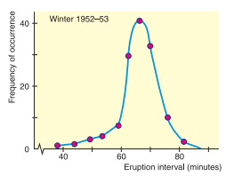
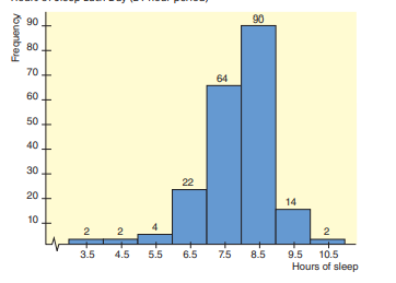
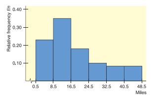
Density curves are smooth curves that can be used to describe the overall pattern of a distribution. Although density curves can come in many different shapes, they all have something in common: The area under any density curve is always equal to one. This is an extremely important concept that we will utilize in this and other chapters. It is usually easier to work with a smooth density curve than a histogram, so we sometimes overlay the density curve onto the histogram to approximate the distribution. A specific type of density curve called a normal curve will be addressed in section 3.2. This “bell-shaped” curve is especially useful in many applications of statistics as you will see later on. We describe density curves in much the same way we describe distributions when using graphs such as histograms or stemplots.
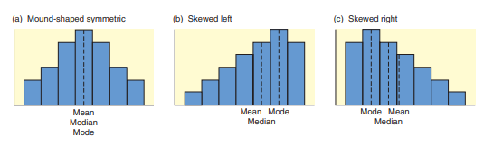
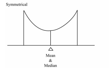
The relationship between the mean and the median is an important concept, especially when dealing with density curves. In a symmetrical density curve, the mean and median will be equal if the distribution is perfectly symmetrical or approximately equal if the distribution is approximately symmetrical. If a distribution is skewed left, then the mean will be “pulled” in the direction of the skewness and will be less than the median. If a distribution is skewed right, the mean is again “pulled” in the direction of the skewness and will be greater than the median. Figure $3.1$ displays distributions that are skewed left, skewed right, and symmetrical. Notice how the mean is “pulled” in the direction of the skewness.

统计代写|AP统计辅导AP统计答疑|Normal Distributions

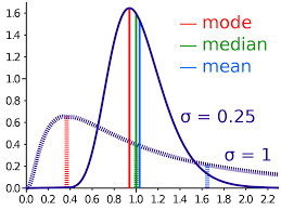
One particular type of density curve that is especially useful in statistics is the normal curve, or normal distribution. Although all normal distributions have the same overall shape, they do differ somewhat depending on the mean and standard deviation of the distribution (Figure 3.3). If we increase or decrease the mean while keeping the standard deviation the same, we will simply shift the distribution to the right or to the left. The more we increase the standard deviation, the “wider” and “shorter” the density curve will be. If we decrease the standard deviation, the density curve will be “narrower” and “taller.” Remember that all density curves, including normal curves, have an area under the curve equal to one. So, no matter what value the mean and standard deviation take, the area under the normal curve is equal to one. This is very important, as you’ll soon see.

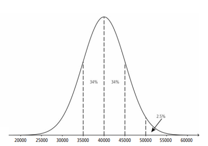
Example 1: Let’s assume that the number of miles that a particular tire will last roughly follows a normal distribution with $\mu=40,000$ miles and $\sigma=5000$ miles. Note that we can use shorthand notation $N(40,000$, 5000 ) to denote a normal distribution with mean equal to 40,000 and standard deviation equal to 5,000 . Since the distribution is not exactly normal but approximately normal, we can assume the distribution will

roughly follow the $68,95,99.7$ Rule. Using the $68,95,99.7$ Rule we can conclude the following (see Figure $3.5$ ):

About $68 \%$ of all tires should last between 35,000 and 45,000 miles $(\mu \pm \sigma)$

About $95 \%$ of all tires should last between 30,000 and 50,000 miles $(\mu \pm 2 \sigma)$

About $99.7 \%$ of all tires should last between 25,000 and 55,000 miles $(\mu \pm 3 \sigma)$

Using the $68,95,99.7$ Rule a little more creatively, we can also conclude:
About $34 \%$ of all tires should last between 40,000 and 45,000 miles.
About $34 \%$ of all tires should last between 35,000 and 40,000 miles.
About $21 / 2 \%$ of all tires should last more than 50,000 miles.
About $84 \%$ of all tires should last less than 45,000 miles.

统计代写|AP统计辅导AP统计答疑|Normal Calculations

Example 2: Referring back to Example 1, let’s suppose that we want to determine the percentage of tires that will last more than 53,400 miles. Recall that we were given $N(40,000,5000)$. To get a more exact answer than we could obtain using the Empirical Rule, we can do the following:
Solution: Always make a sketch! (See Figure 3.6.)

Using substitution, we obtain $z=\frac{53,400-40,000}{5000}=2.68$
Notice that the formula for $z$ takes the difference of $x$ and $\mu$ and divides it by $\sigma$. Thus, a z-score is the number of standard deviations that $x$ lies above or below the mean. So, 53,400 is $2.68$ standard deviations above the mean. You should always get a positive value for $z$ if the value of $x$ is above the mean, and a negative value for $z$ if the value of $x$ is below the mean.
When we find the z-score, we are standardizing the values of the distribution. Since these values are values of a normal distribution, the distribution we obtain is called the standard normal distribution. This new distribution, the standard normal distribution, has a mean of zero and a standard deviation of one. We can then write $N(0,1)$
The advantage of standardizing any given normal distribution to the standard normal distribution is that we can now find the area under the curve for any given value of $x$ that is needed.

We can now use the z-score of $2.68$ that we obtained earlier. Using Table A, we can look up the area to the left of $z=2.68$. Notice that Table A has two sides – one for positive values for $z$ and the other for negative values for $z$. Using the side of the table with the positive values for $z$, follow the left-hand column down until you reach $2.6$. Then go across the top of the table until you reach $.08$. By crossreferencing $2.6$ and $.08$, we can obtain the area to the left of $z=2.68$, which is $0.9963$.

In other words, $99.63 \%$ of tires will last less than 53,400 miles. We want to know what percent of tires will last more than 53,400 miles, so we subtract $0.9963$ from 1. Remember that the total area under any density curve is equal to one.
We obtain $1-0.9963=0.0037$.

统计代写|AP统计辅导AP统计答疑|Density Curves

密度曲线是可用于描述分布的整体模式的平滑曲线。尽管密度曲线可以有许多不同的形状，但它们都有一个共同点：任何密度曲线下的面积总是等于一。这是一个非常重要的概念，我们将在本章和其他章节中使用。使用平滑的密度曲线通常比使用直方图更容易，因此我们有时将密度曲线叠加到直方图上以近似分布。3.2 节将介绍一种称为正态曲线的特定类型的密度曲线。这种“钟形”曲线在许多统计应用中特别有用，您将在后面看到。我们描述密度曲线的方式与我们在使用直方图或茎图等图形时描述分布的方式非常相似。
平均值和中位数之间的关系是一个重要的概念，尤其是在处理密度曲线时。在对称密度曲线中，如果分布完全对称，则平均值和中位数将相等，如果分布近似对称，则平均值和中位数将近似相等。如果分布向左偏，则均值将被“拉”向偏斜方向，并且将小于中位数。如果分布向右偏斜，则均值再次向偏斜方向“拉动”，并将大于中位数。数字3.1显示左偏、右偏和对称的分布。请注意均值是如何向偏度方向“拉动”的。

统计代写|AP统计辅导AP统计答疑|Normal Distributions

在统计学中特别有用的一种特殊类型的密度曲线是正态曲线或正态分布。尽管所有正态分布的总体形状都相同，但它们确实有所不同，具体取决于分布的均值和标准差（图 3.3）。如果我们在保持标准差不变的情况下增加或减少均值，我们将简单地将分布向右或向左移动。我们增加的标准差越多，密度曲线就会越“宽”和“短”。如果我们减小标准偏差，密度曲线将“更窄”和“更高”。请记住，所有密度曲线，包括正态曲线，曲线下的面积都等于 1。因此，无论均值和标准差取什么值，正态曲线下的面积都等于 1。

示例 1：假设特定轮胎的续航里程大致遵循正态分布，其中μ=40,000英里和σ=5000英里。请注意，我们可以使用速记符号ñ(40,000, 5000 ) 表示均值等于 40,000 且标准差等于 5,000 的正态分布。由于分布不是完全正态分布而是近似正态分布，我们可以假设分布将

大致按照68,95,99.7规则。使用68,95,99.7规则我们可以得出以下结论（见图3.5 ):

关于68%所有轮胎的使用寿命应在 35,000 到 45,000 英里之间(μ±σ)

关于95%所有轮胎的使用寿命应在 30,000 到 50,000 英里之间(μ±2σ)

关于99.7%所有轮胎的使用寿命应在 25,000 到 55,000 英里之间(μ±3σ)

使用68,95,99.7更有创意地规则一点，我们也可以得出结论：
关于34%所有轮胎的使用寿命应在 40,000 到 45,000 英里之间。
关于34%所有轮胎的使用寿命应在 35,000 到 40,000 英里之间。
关于21/2%所有轮胎的使用寿命应超过 50,000 英里。
关于84%所有轮胎的使用寿命应少于 45,000 英里。

统计代写|AP统计辅导AP统计答疑|Normal Calculations

示例 2：回到示例 1，假设我们要确定能够持续超过 53,400 英里的轮胎的百分比。回想一下，我们得到了ñ(40,000,5000). 为了得到比我们使用经验法则获得的更准确的答案，我们可以执行以下操作：
解决方案：总是画草图！（见图 3.6。）

使用替换，我们得到和=53,400−40,0005000=2.68
请注意，公式为和取差异X和μ并将其除以σ. 因此，z 分数是标准差的数量X高于或低于平均值。所以，53,400 是2.68高于平均值的标准差。你应该总是得到一个正值和如果值X高于平均值，并且为负值和如果值X低于平均值。
当我们找到 z 分数时，我们正在标准化分布的值。由于这些值是正态分布的值，我们得到的分布称为标准正态分布。这个新分布，即标准正态分布，均值为 0，标准差为 1。然后我们可以写ñ(0,1)
将任何给定的正态分布标准化为标准正态分布的优点是我们现在可以找到任何给定值的曲线下面积X这是需要的。

我们现在可以使用 z-score2.68我们之前获得的。使用表 A，我们可以查找左侧的区域和=2.68. 请注意，表 A 有两个方面 – 一个用于正值和另一个用于负值和. 使用带有正值的表格一侧和, 沿着左列向下直到到达2.6. 然后穿过桌子的顶部，直到到达.08. 通过交叉引用2.6和.08，我们可以得到左边的区域和=2.68，即0.9963.

换句话说，99.63%的轮胎将持续不到 53,400 英里。我们想知道有多少百分比的轮胎将持续超过 53,400 英里，所以我们减去0.9963从 1. 请记住，任何密度曲线下的总面积都等于 1。
我们获得1−0.9963=0.0037.

统计代写请认准statistics-lab™. statistics-lab™为您的留学生涯保驾护航。

金融工程代写

金融工程是使用数学技术来解决金融问题。金融工程使用计算机科学、统计学、经济学和应用数学领域的工具和知识来解决当前的金融问题，以及设计新的和创新的金融产品。

非参数统计代写

非参数统计指的是一种统计方法，其中不假设数据来自于由少数参数决定的规定模型；这种模型的例子包括正态分布模型和线性回归模型。

广义线性模型代考

广义线性模型（GLM）归属统计学领域，是一种应用灵活的线性回归模型。该模型允许因变量的偏差分布有除了正态分布之外的其它分布。

术语广义线性模型（GLM）通常是指给定连续和/或分类预测因素的连续响应变量的常规线性回归模型。它包括多元线性回归，以及方差分析和方差分析（仅含固定效应）。

有限元方法代写

有限元方法（FEM）是一种流行的方法，用于数值解决工程和数学建模中出现的微分方程。典型的问题领域包括结构分析、传热、流体流动、质量运输和电磁势等传统领域。

有限元是一种通用的数值方法，用于解决两个或三个空间变量的偏微分方程（即一些边界值问题）。为了解决一个问题，有限元将一个大系统细分为更小、更简单的部分，称为有限元。这是通过在空间维度上的特定空间离散化来实现的，它是通过构建对象的网格来实现的：用于求解的数值域，它有有限数量的点。边界值问题的有限元方法表述最终导致一个代数方程组。该方法在域上对未知函数进行逼近。[1] 然后将模拟这些有限元的简单方程组合成一个更大的方程系统，以模拟整个问题。然后，有限元通过变化微积分使相关的误差函数最小化来逼近一个解决方案。

tatistics-lab作为专业的留学生服务机构，多年来已为美国、英国、加拿大、澳洲等留学热门地的学生提供专业的学术服务，包括但不限于Essay代写，Assignment代写，Dissertation代写，Report代写，小组作业代写，Proposal代写，Paper代写，Presentation代写，计算机作业代写，论文修改和润色，网课代做，exam代考等等。写作范围涵盖高中，本科，研究生等海外留学全阶段，辐射金融，经济学，会计学，审计学，管理学等全球99%专业科目。写作团队既有专业英语母语作者，也有海外名校硕博留学生，每位写作老师都拥有过硬的语言能力，专业的学科背景和学术写作经验。我们承诺100%原创，100%专业，100%准时，100%满意。

随机分析代写

随机微积分是数学的一个分支，对随机过程进行操作。它允许为随机过程的积分定义一个关于随机过程的一致的积分理论。这个领域是由日本数学家伊藤清在第二次世界大战期间创建并开始的。

时间序列分析代写

随机过程，是依赖于参数的一组随机变量的全体，参数通常是时间。随机变量是随机现象的数量表现，其时间序列是一组按照时间发生先后顺序进行排列的数据点序列。通常一组时间序列的时间间隔为一恒定值（如1秒，5分钟，12小时，7天，1年），因此时间序列可以作为离散时间数据进行分析处理。研究时间序列数据的意义在于现实中，往往需要研究某个事物其随时间发展变化的规律。这就需要通过研究该事物过去发展的历史记录，以得到其自身发展的规律。

回归分析代写

多元回归分析渐进（Multiple Regression Analysis Asymptotics）属于计量经济学领域，主要是一种数学上的统计分析方法，可以分析复杂情况下各影响因素的数学关系，在自然科学、社会和经济学等多个领域内应用广泛。

MATLAB代写

MATLAB 是一种用于技术计算的高性能语言。它将计算、可视化和编程集成在一个易于使用的环境中，其中问题和解决方案以熟悉的数学符号表示。典型用途包括：数学和计算算法开发建模、仿真和原型制作数据分析、探索和可视化科学和工程图形应用程序开发，包括图形用户界面构建MATLAB 是一个交互式系统，其基本数据元素是一个不需要维度的数组。这使您可以解决许多技术计算问题，尤其是那些具有矩阵和向量公式的问题，而只需用 C 或 Fortran 等标量非交互式语言编写程序所需的时间的一小部分。MATLAB 名称代表矩阵实验室。MATLAB 最初的编写目的是提供对由 LINPACK 和 EISPACK 项目开发的矩阵软件的轻松访问，这两个项目共同代表了矩阵计算软件的最新技术。MATLAB 经过多年的发展，得到了许多用户的投入。在大学环境中，它是数学、工程和科学入门和高级课程的标准教学工具。在工业领域，MATLAB 是高效研究、开发和分析的首选工具。MATLAB 具有一系列称为工具箱的特定于应用程序的解决方案。对于大多数 MATLAB 用户来说非常重要，工具箱允许您学习和应用专业技术。工具箱是 MATLAB 函数（M 文件）的综合集合，可扩展 MATLAB 环境以解决特定类别的问题。可用工具箱的领域包括信号处理、控制系统、神经网络、模糊逻辑、小波、仿真等。

R语言代写	问卷设计与分析代写
PYTHON代写	回归分析与线性模型代写
MATLAB代写	方差分析与试验设计代写
STATA代写	机器学习/统计学习代写
SPSS代写	计量经济学代写
EVIEWS代写	时间序列分析代写
EXCEL代写	深度学习代写
SQL代写	各种数据建模与可视化代写

统计代写|AP统计辅导AP统计答疑|Exploring and Graphing Bivariate Data

Posted on 2022年5月19日2022年5月19日 by statistics-lab

如果你也在怎样代写AP统计这个学科遇到相关的难题，请随时右上角联系我们的24/7代写客服。

我们提供的AP统计及其相关学科的代写，服务范围广, 其中包括但不限于:

Statistical Inference 统计推断
Statistical Computing 统计计算
Advanced Probability Theory 高等概率论
Advanced Mathematical Statistics 高等数理统计学
(Generalized) Linear Models 广义线性模型
Statistical Machine Learning 统计机器学习
Longitudinal Data Analysis 纵向数据分析
Foundations of Data Science 数据科学基础

统计代写|AP统计辅导AP统计答疑|Exploring and Graphing Bivariate Data

统计代写|AP统计辅导AP统计答疑|Scatterplots

Scatterplots are ideal for exploring the relationship between two quantitative variables. When constructing a scatterplot we often deal with explanatory and response variables. The explanatory variable may be thought of as the independent variable, and the response variable may be thought of as the dependent variable.
It’s important to note that when working with two quantitative variables, we do not always consider one to be the explanatory variable and the other to be the response variable. Sometimes, we just want to explore the relationship between two variables, and it doesn’t make sense to declare one variable the explanatory and the other the response.
We interpret scatterplots in much the same way we interpret univariate data; we look for the overall pattern of the data. We address the form, direction, and strength of the relationship. Remember to look for outliers as well. Are there any points in the scatterplot that deviate from the overall pattern?
When addressing the form of the relationship, look to see if the data is linear (Figure 2.1) or curved (Figure 2.2).

统计代写|AP统计辅导AP统计答疑|Correlation

When dealing with linear relationships, we often use the r-value, or the correlation coefficient. The correlation coefficient can be found by using the formula:
$$
r=\frac{1}{n-1} \sum\left(\frac{x_{i}-\bar{x}}{s_{x}}\right)\left(\frac{y_{i}-\bar{y}}{s_{y}}\right)
$$
In practice, we avoid using the formula at all cost. However, it helps to suffer through a couple of calculations using the formula in order to understand how the formula works and gain a deeper appreciation of technology.
Facts about Correlation
It’s important to remember the following facts about correlation (make sure you know all of them!):

Correlation (the r-value) only describes a linear relationship. Do not use $r$ to describe a curved relationship.

Correlation makes no distinction between explanatory and response variables. If we switch the $x$ and $y$ variables, we still get the same correlation.
Correlation has no unit of measurement. The formula for correlation uses the means and standard deviations for $x$ and $y$ and thus uses standardized values.

If $r$ is positive, then the association is positive; if $r$ is negative, then the association is negative.
$-1 \leq r \leq 1: r=1$ implies that there is a perfectly linear positive
relationship. $r=-1$ implies that there is a perfectly linear negative relationship. $r=0$ implies that there is no correlation.

The r-value, like the mean and standard deviation, is not a resistant measure. This means that even one extreme data point can have a dramatic effect on the r-value. Remember that outliers can either strengthen or weaken the r-value. So use caution!
The r-value does not change when you change units of measurement. For example, changing the $x$ and/or $y$ variables from centimeters to millimeters or even from centimeters to inches does not change the r-value.

Correlation does not imply causation. Just because two variables are strongly associated or even correlated (linear) does not mean that changes in one variable are causing changes in another.

统计代写|AP统计辅导AP统计答疑|Least Squares Regression

When modeling linear data, we use the Least Squares Regression Line (LSRL). The LSRL is fitted to the data by minimizing the sum of the squared residuals. The graphing calculator again comes to our rescue by calculating the LSRL and its equation. The LSRL equation takes the form of $\hat{y}=a+b x$ where $b$ is the slope and $a$ is the $y$-intercept. The AP* formula sheet uses the form $\hat{y}=b_{0}+b_{1} x$. Either form may be used as long as you define your variables. Just remember that the number in front of $x$ is the slope, and the “other” number is the $y$-intercept.
Once the LSRL is fitted to the data, we can then use the LSRL equation to make predictions. We can simply substitute a value of $x$ into the equation of the LSRL and obtain the predicted value, $\hat{y}$.
The LSRL minimizes the sum of the squared residuals. What does this mean? A residual is the difference between the observed value, $y$, and the predicted value, $\hat{y}$. In other words, residual-observed – predicted. Remember that all predicted values are located on the LSRL. A residual can be positive, negative, or zero. A residual is zero only when the point is located on the LSRL. Since the sum of the residuals is always zero,

we square the vertical distances of the residuals. The LSRL is fitted to the data so that the sum of the square of these vertical distances is as small as possible.

The slope of the regression line (LSRL) is important. Consider the time required to run the last mile of a marathon in relation to the time required to run the first mile of a marathon. The equation $\hat{y}=1.25 x$, where $x$ is the time required to run the first mile in minutes and $\hat{y}$ is the predicted time it takes to run the last mile in minutes, could be used to model or predict the runner’s time for his last mile. The interpretation of the slope in context would be that for every one minute increase in time needed to run the first mile, the predicted time to run the last mile would increase by $1.25$ minutes, on average. It should be noted that the slope is a rate of change and that that since the slope is positive, the time will increase by $1.25$ minutes. A negative slope would give a negative rate of change.

AP统计代写

统计代写|AP统计辅导AP统计答疑|Scatterplots

散点图非常适合探索两个定量变量之间的关系。在构建散点图时，我们经常处理解释变量和响应变量。解释变量可以被认为是自变量，而响应变量可以被认为是因变量。
需要注意的是，在处理两个定量变量时，我们并不总是将一个视为解释变量，而将另一个视为响应变量。有时，我们只是想探索两个变量之间的关系，而将一个变量声明为解释变量，另一个变量声明为响应变量是没有意义的。
我们解释散点图的方式与解释单变量数据的方式大致相同；我们寻找数据的整体模式。我们解决关系的形式、方向和强度。记住也要寻找异常值。散点图中是否有任何点偏离整体模式？
在处理关系的形式时，查看数据是线性的（图 2.1）还是曲线的（图 2.2）。

统计代写|AP统计辅导AP统计答疑|Correlation

在处理线性关系时，我们经常使用 r 值，或相关系数。相关系数可以通过使用公式找到：
r=1n−1∑(X一世−X¯sX)(是一世−是¯s是)
在实践中，我们不惜一切代价避免使用该公式。但是，它有助于使用公式进行几次计算，以了解公式的工作原理并更深入地了解技术。
关于相关性的事实
记住以下有关相关性的事实很重要（确保您了解所有这些事实！）：

相关性（r 值）仅描述线性关系。不使用r来描述弯曲的关系。

相关性不区分解释变量和响应变量。如果我们切换X和是变量，我们仍然得到相同的相关性。
相关性没有度量单位。相关性公式使用平均值和标准差X和是因此使用标准化值。

如果r为正，则关联为正；如果r为负，则关联为负。
−1≤r≤1:r=1意味着存在完全线性的正
相关。r=−1意味着存在完全线性的负相关。r=0表示没有相关性。

r 值与均值和标准差一样，不是一种抗性测量。这意味着即使是一个极端数据点也会对 r 值产生巨大影响。请记住，异常值可以加强或削弱 r 值。所以要小心！
更改测量单位时，r 值不会更改。例如，改变X和/或是从厘米到毫米甚至从厘米到英寸的变量不会改变 r 值。

相关性并不意味着因果关系。仅仅因为两个变量强相关甚至相关（线性）并不意味着一个变量的变化会导致另一个变量的变化。

统计代写|AP统计辅导AP统计答疑|Least Squares Regression

在对线性数据建模时，我们使用最小二乘回归线 (LSRL)。LSRL 通过最小化残差平方和来拟合数据。图形计算器通过计算 LSRL 及其方程再次帮助我们。LSRL 方程的形式为是^=一种+bX在哪里b是斜率和一种是个是-截距。AP* 公式表使用表格是^=b0+b1X. 只要您定义了变量，就可以使用任何一种形式。只要记住前面的数字X是斜率，“其他”数字是是-截距。
一旦将 LSRL 拟合到数据中，我们就可以使用 LSRL 方程进行预测。我们可以简单地替换一个值X代入LSRL的方程，得到预测值，是^.
LSRL 最小化残差平方和。这是什么意思？残差是观察值之间的差异，是, 和预测值,是^. 换句话说，残差观察 – 预测。请记住，所有预测值都位于 LSRL 上。残差可以是正数、负数或零。只有当点位于 LSRL 上时，残差才为零。由于残差之和始终为零，

我们将残差的垂直距离平方。LSRL 适合数据，以便这些垂直距离的平方和尽可能小。

回归线的斜率 (LSRL) 很重要。考虑跑完马拉松最后一英里所需的时间与跑完马拉松第一英里所需的时间。方程是^=1.25X，在哪里X是跑第一英里所需的时间，以分钟为单位，并且是^是以分钟为单位运行最后一英里的预测时间，可用于建模或预测跑步者最后一英里的时间。在上下文中对斜率的解释是，跑第一英里所需的时间每增加一分钟，跑最后一英里的预测时间将增加1.25分钟，平均。应该注意的是斜率是一个变化率，由于斜率为正，时间将增加1.25分钟。负斜率将产生负变化率。

统计代写请认准statistics-lab™. statistics-lab™为您的留学生涯保驾护航。

金融工程代写

非参数统计代写

非参数统计指的是一种统计方法，其中不假设数据来自于由少数参数决定的规定模型；这种模型的例子包括正态分布模型和线性回归模型。

广义线性模型代考

广义线性模型（GLM）归属统计学领域，是一种应用灵活的线性回归模型。该模型允许因变量的偏差分布有除了正态分布之外的其它分布。

有限元方法代写

随机分析代写

时间序列分析代写

回归分析代写

MATLAB代写

R语言代写	问卷设计与分析代写
PYTHON代写	回归分析与线性模型代写
MATLAB代写	方差分析与试验设计代写
STATA代写	机器学习/统计学习代写
SPSS代写	计量经济学代写
EVIEWS代写	时间序列分析代写
EXCEL代写	深度学习代写
SQL代写	各种数据建模与可视化代写

统计代写|AP统计辅导AP统计答疑|Exploring and Graphing Univariate Data

Posted on 2022年5月19日2022年5月19日 by statistics-lab

如果你也在怎样代写AP统计这个学科遇到相关的难题，请随时右上角联系我们的24/7代写客服。

我们提供的AP统计及其相关学科的代写，服务范围广, 其中包括但不限于:

Statistical Inference 统计推断
Statistical Computing 统计计算
Advanced Probability Theory 高等概率论
Advanced Mathematical Statistics 高等数理统计学
(Generalized) Linear Models 广义线性模型
Statistical Machine Learning 统计机器学习
Longitudinal Data Analysis 纵向数据分析
Foundations of Data Science 数据科学基础

统计代写|AP统计辅导AP统计答疑|Exploring and Graphing Univariate Data

统计代写|AP统计辅导AP统计答疑|Describing Distributions

The organization of data into graphical displays is essential to understanding statistics. This chapter discusses how to describe distributions and various types of graphs used for organizing univariate data. The types of graphs include modified boxplots, histograms, stem-and-leaf plots, bar graphs, dotplots, and pie charts. Students in AP Statistics should have a clear understanding of what a variable is and the types of variables that are encountered.
A variable is a characteristic of an individual and can take on different values for different individuals. Two types of variables are discussed in this chapter: categorical variables and quantitative variables.

Categorical variable: Places an individual into a category or group Quantitative variable: Takes on a numerical value

Variables may take on different values. The pattern of variation of a variable is its distribution. The distribution of a variable tells us what values the variable takes and how often it takes each value.

When describing distributions, it’s important to describe what you see in the graph. It’s important to address the shape, center, and spread of the distribution in the context of the problem.
When describing shape, focus on the main features of the distribution. Is the graph approximately symmetrical, skewed left, or skewed right?

统计代写|AP统计辅导AP统计答疑|Standard Deviation

$$
s=\sqrt{2.5} \approx 1.5811
$$
It’s probably more important to understand the concept of what standard deviation means than to be able to calculate it by hand. Our trusty calculators or computer software can handle the calculation for us. Understanding what the number means is what’s most important. It’s worth noting that most calculators will give two values for standard deviation. One is used when dealing with a population, and the other is used when dealing with a sample. The TI $83 / 84$ calculator shows the population standard deviation as $x$ and the sample standard deviation as $S_{x}$. A population is all individuals of interest, and a sample is just part of a population. We’ll discuss the concept of population and different types of samples in later chapters.

It’s also important to address any outliers that might be present in the distribution. Outliers are values that fall outside the overall pattern of the distribution. It is important to be able to identify potential outliers in a distribution, but we also want to determine whether or not a value is mathematically an outlier.
Example 4: Consider Data Set B, which consists of test scores from a college statistics course:
$$
\begin{aligned}
&98,36,67,85,79,100,88,85,60,69,93,58,65,89,88,71,79,85,73,87, \
&81,77,76,75,76,73
\end{aligned}
$$

Arrange the data in ascending order.
$$
\begin{aligned}
&36,58,60,65,67,69,71,73,73,75,76,76,77,79,79,81,85,85,85,87, \
&88,88,89,93,98,100
\end{aligned}
$$Find the median (average of the two middle numbers): 78 .
Find the median of the first half of numbers. This is the first quartile, $\mathrm{Q}_{1}: 71$.
Find the median of the second half of numbers, the third quartile, $\mathrm{Q}_{3}: 87$.
Find the interquartile range (IQR): $I Q R=Q_{3}-Q_{1}=87-71=16$.
Multiply the IQR by $1.5: 16 \times 1.5=24$.
Add this number to $Q_{3}$ and subtract this number from $Q_{1}$. $87+24=111$ and $71-24=47$
Any number smaller than 47 or larger than 111 would be considered an outlier. Therefore, 36 is the only outlier in this set.

统计代写|AP统计辅导AP统计答疑|Modified Boxplots

Modified boxplots are extremely useful in AP Statistics. A modified boxplot is ideal when you are interested in checking a distribution for outliers or skewness, which will be essential in later chapters. To construct a modified boxplot, we use the five-number summary. The box of the modified boxplot consists of $\mathrm{Q} 1, \mathrm{M}$, and $\mathrm{Q} 3$. Outliers are marked as separate points. The tails of the plot consist of either the smallest and largest numbers or the smallest and largest numbers that are not considered outliers by our mathematical criterion discussed earlier. Outliers appear as separate dots or asterisks. Modified boxplots can be constructed with ease using the graphing calculator or computer software. Be sure to use the modified boxplot instead of the regular boxplot, since we are usually interested in knowing if outliers are present. Side-by-side boxplots can be used to make visual comparisons between two or more distributions. Figure $1.4$ displays the test scores from Data Set B. Notice that the test score of 36 (which is an outlier) is represented using a separate point.

Histograms are also useful for displaying distributions when the variable of interest is numeric (Figure 1.5). When the variable is categorical, the graph is called a bar chart or bar graph. The bars of the histogram should be touching and should be of equal width. The heights of the bars represent the frequency or relative frequency. As with modified boxplots, histograms can be easily constructed using the TI-83/84 graphing calculator or computer software. With some minor adjustments to the window of the graphing calculator, we can easily transfer the histogram from calculator to paper. We often use the ZoomStat function of the TI-83/84 graphing calculator to create histograms. ZoomStat will fit the data to the screen of the graphing calculator and often creates bars with non-integer dimensions. In order to create histograms that have integer dimensions, we must make adjustments to the window of the graphing calculator. Once these adjustments have been made, we can then easily copy the calculator histogram onto paper. Histograms are especially useful in finding the shape of a distribution. To find the center of the histogram, as measured by the median, find the line that would divide the histogram into two equal parts. To find the mean of the distributions, locate the balancing point of the histogram.

AP统计代写

统计代写|AP统计辅导AP统计答疑|Describing Distributions

将数据组织成图形显示对于理解统计数据至关重要。本章讨论如何描述用于组织单变量数据的分布和各种类型的图。图表的类型包括修改后的箱线图、直方图、茎叶图、条形图、点图和饼图。AP统计学的学生应该清楚地了解变量是什么以及遇到的变量类型。
变量是个体的特征，对于不同的个体可以取不同的值。本章讨论了两类变量：分类变量和定量变量。

分类变量：将个人置于一个类别或组中定量变量：采用数值

变量可能具有不同的值。变量的变化模式是它的分布。变量的分布告诉我们变量取什么值以及取每个值的频率。

在描述分布时，描述您在图表中看到的内容很重要。在问题的上下文中解决分布的形状、中心和分布很重要。
在描述形状时，请关注分布的主要特征。图形是近似对称的、向左倾斜还是向右倾斜？

统计代写|AP统计辅导AP统计答疑|Standard Deviation

s=2.5≈1.5811
理解标准差的含义可能比手动计算更重要。我们值得信赖的计算器或计算机软件可以为我们处理计算。了解数字的含义是最重要的。值得注意的是，大多数计算器会给出两个标准差值。一种用于处理总体，另一种用于处理样本。TI83/84计算器将总体标准差显示为X样本标准差为小号X. 总体是所有感兴趣的个体，样本只是总体的一部分。我们将在后面的章节中讨论总体的概念和不同类型的样本。

解决分布中可能存在的任何异常值也很重要。异常值是不属于分布的整体模式的值。能够识别分布中的潜在异常值很重要，但我们还想确定一个值在数学上是否是异常值。
示例 4：考虑数据集 B，它由大学统计学课程的考试成绩组成：
98,36,67,85,79,100,88,85,60,69,93,58,65,89,88,71,79,85,73,87, 81,77,76,75,76,73

按升序排列数据。
36,58,60,65,67,69,71,73,73,75,76,76,77,79,79,81,85,85,85,87, 88,88,89,93,98,100求中位数（两个中间数的平均值）： 78 。
求数字前半部分的中位数。这是第一个四分位数，问1:71.
找到数字后半部分的中位数，第三个四分位数，问3:87.
求四分位距 (IQR)：一世问R=问3−问1=87−71=16.
将 IQR 乘以1.5:16×1.5=24.
将此号码添加到问3并从中减去这个数字问1. 87+24=111和71−24=47
任何小于 47 或大于 111 的数字都将被视为异常值。因此，36 是该集合中唯一的异常值。

统计代写|AP统计辅导AP统计答疑|Modified Boxplots

修改后的箱线图在 AP 统计中非常有用。当您有兴趣检查异常值或偏度的分布时，修改后的箱线图是理想的选择，这在后面的章节中是必不可少的。为了构建修改后的箱线图，我们使用五数摘要。修改后的箱线图的箱由问1,米，和问3. 异常值被标记为单独的点。该图的尾部由我们前面讨论的数学标准不认为是异常值的最小和最大数字或最小和最大数字组成。异常值显示为单独的点或星号。使用图形计算器或计算机软件可以轻松构建修改后的箱线图。请务必使用修改后的箱线图而不是常规箱线图，因为我们通常有兴趣知道是否存在异常值。并排箱线图可用于在两个或多个分布之间进行视觉比较。数字1.4显示来自数据集 B 的测试分数。请注意，测试分数 36（这是一个异常值）使用单独的点表示。

当感兴趣的变量是数字时，直方图也可用于显示分布（图 1.5）。当变量是分类变量时，图形称为条形图或条形图。直方图的条应该是接触的并且应该是相等的宽度。条的高度代表频率或相对频率。与修改后的箱线图一样，可以使用 TI-83/84 图形计算器或计算机软件轻松构建直方图。通过对图形计算器窗口的一些细微调整，我们可以轻松地将直方图从计算器转移到纸上。我们经常使用 TI-83/84 图形计算器的 ZoomStat 功能来创建直方图。ZoomStat 将使数据适合图形计算器的屏幕，并经常创建具有非整数尺寸的条形图。为了创建具有整数维度的直方图，我们必须对图形计算器的窗口进行调整。一旦进行了这些调整，我们就可以轻松地将计算器直方图复制到纸上。直方图在寻找分布形状时特别有用。要找到直方图的中心（按中值测量），请找到将直方图分成两个相等部分的线。要找到分布的平均值，请找到直方图的平衡点。找到将直方图分成两个相等部分的线。要找到分布的平均值，请找到直方图的平衡点。找到将直方图分成两个相等部分的线。要找到分布的平均值，请找到直方图的平衡点。

统计代写请认准statistics-lab™. statistics-lab™为您的留学生涯保驾护航。

金融工程代写

非参数统计代写

非参数统计指的是一种统计方法，其中不假设数据来自于由少数参数决定的规定模型；这种模型的例子包括正态分布模型和线性回归模型。

广义线性模型代考

广义线性模型（GLM）归属统计学领域，是一种应用灵活的线性回归模型。该模型允许因变量的偏差分布有除了正态分布之外的其它分布。

有限元方法代写

随机分析代写

时间序列分析代写

回归分析代写

MATLAB代写

R语言代写	问卷设计与分析代写
PYTHON代写	回归分析与线性模型代写
MATLAB代写	方差分析与试验设计代写
STATA代写	机器学习/统计学习代写
SPSS代写	计量经济学代写
EVIEWS代写	时间序列分析代写
EXCEL代写	深度学习代写
SQL代写	各种数据建模与可视化代写

统计代写|AP统计作业代写代考|Probability Theory

Posted on 2022年4月13日2022年4月13日 by statistics-lab

如果你也在怎样代写AP统计这个学科遇到相关的难题，请随时右上角联系我们的24/7代写客服。

AP 统计主要是介绍收集、分析和从数据中得出结论的主要概念和工具。

statistics-lab™ 为您的留学生涯保驾护航在代写AP统计方面已经树立了自己的口碑, 保证靠谱, 高质且原创的统计Statistics代写服务。我们的专家在代写AP统计方面经验极为丰富，各种代写AP统计相关的作业也就用不着说。

我们提供的AP统计及其相关学科的代写，服务范围广, 其中包括但不限于:

Statistical Inference 统计推断
Statistical Computing 统计计算
Advanced Probability Theory 高等楖率论
Advanced Mathematical Statistics 高等数理统计学
(Generalized) Linear Models 广义线性模型
Statistical Machine Learning 统计机器学习
Longitudinal Data Analysis 纵向数据分析
Foundations of Data Science 数据科学基础

统计代写|AP统计作业代写代考|How Often Do Lie Detectors Lie?

James Burke is an educator who is known for his interesting science-related radio and television shows aired by the British Broadcasting Corporation. His book Chances: Risk and Odds in Everyday Life (Virginia Books, London) contains a great wealth of fascinating information about probabilities. The following quote is from Professor Burke’s book:
If I take a polygraph test and lie, what is the risk I will be detected? According to some studies, there’s about a 72 percent chance you will be caught by the machine.

What is the risk that if I take a polygraph test it will incorrectly say that $I$ lied? At least 1 in 15 will be thus falsely accused.
Both of these statements contain conditional probabilities, which we will study in Section 4.2. Information from that section will enable us to answer the following:
Suppose a person answers $10 \%$ of a long battery of questions with lies. Assume that the remaining $90 \%$ of the questions are answered truthfully.

Estimate the percentage of answers the polygraph will wrongly indicate as lies.
Estimate the percentage of answers the polygraph will correctly indicate as lies.

If the polygraph indicated that $30 \%$ of the questions were answered as lies, what would you estimate for the actual percentage of questions the person answered as lies? (See Problems 27 and 28 in Section 4.2.)

统计代写|AP统计作业代写代考|Probability Assignment

Consider each of the following events, and determine how the probability is assigned.
(a) A sports announcer claims that Sheila has a $90 \%$ chance of breaking the world record in the 100-yard dash.
SOLUTION: It is likely the sports announcer used intuition based on Sheila’s past performance.
Section 4.1 What is Probability? 145
(b) Henry figures that if he guesses on a true-false question, the probability of getting it right is $0.50$.
sOLUTION: In this case there are two possible outcomes: Henry’s answer is either correct or incorrect. Since Henry is guessing, we assume the outcomes are equally likely. There are $n=2$ equally likely outcomes, and only one is correct. By formula (2),
$$
P(\text { correct answer })=\frac{\text { Number of favorable outcomes }}{\text { Total number of outcomes }}=\frac{1}{2}=0.50
$$
(c) The Right to Health lobby claims that the probability of getting an erroneous medical laboratory report is $0.40$, based on a random sample of 200 laboratory reports, of which 80 were erroneous.
soLUTION: Formula (1) for relative frequency gives the probability, with sample size $n=200$ and number of errors $f=80$.
$$
P(\text { error })=\text { relative frequency }=\frac{f}{n}=\frac{80}{200}=0.40
$$

统计代写|AP统计作业代写代考|Using a Sample Space

Human eye color is controlled by a single pair of genes (one from the father and one from the mother) called a genotype. Brown eye color, $\mathrm{B}$, is dominant over blue eye color, $\ell$. Therefore, in the genotype $\mathrm{B} \ell$, consisting of one brown gene $\mathrm{B}$ and one blue gene $\ell$, the brown gene dominates. A person with a $\mathrm{B} \ell$ genotype has brown eyes.
If both parents have brown eyes and have genotype $\mathrm{B} \ell$, what is the probability that their child will have blue eyes? What is the probability the child will have brown eyes?

SOLUTION: To answer these questions, we need to look at the sample space of all possible eye-color genotypes for the child. They are given in Table 4-1.
TABLE 4-1 Eye Color Genotypes for Child
\begin{tabular}{lll}
\hline & \multicolumn{2}{c}{ Mother } \
\cline { 2 – 3 } Father & B & $\ell$ \
\hline B & BB & $B \ell$ \
$\ell$ & $\ell B$ & $\ell \ell$ \
\hline
\end{tabular}
According to genetics theory, the four possible genotypes for the child are equally likely. Therefore, we can use Formula (2) to compute probabilities. Blue eyes can occur only with the $\ell \ell$ genotype, so there is only one outcome favorable to blue eyes. By formula (2),
$$
P(\text { blue eyes })=\frac{\text { Number of favorable outcomes }}{\text { Total number of outcomes }}=\frac{1}{4}
$$
Brown eyes occur with the three remaining genotypes: $B B, B \ell$, and $\ell B$. By formula (2),
$$
P(\text { brown eyes })=\frac{\text { Number of favorable outcomes }}{\text { Total number of outcomes }}=\frac{3}{4}
$$

There is another important point about probability assignments of simple events.
The sum of the probabilities of all simple events in a sample space must equal $1 .$
We can use this fact to determine the probability that an event will not occur. For instance, if you think the probability is $0.65$ that you will win a tennis match, you assume the probability is $0.35$ that your opponent will win.

The complement of an event $A$ is the event that $A$ does not occur. We use the notation $A^{c}$ to designate the complement of event $A$. Figure 41 shows the event $A$ and its complement $A^{c}$. In the literature, the symbols $A^{\circ}$ and $\bar{A}$ are also used to designate the complement of event $A$

Noticéc that the two distinet events $A$ ând $A^{2}$ make up the entire samplec spăce. Therefore, the sum of their probabilities is 1 .
The complement of event $A$ is the event that $A$ does not occur. $A^{c}$ designates the complement of event $A$. Furthermore,

$P(A)+P\left(A^{c}\right)=1$
$P($ event $A$ does not occur $)=P\left(A^{c}\right)=1-P(A)$

AP统计代写

统计代写|AP统计作业代写代考|How Often Do Lie Detectors Lie?

詹姆斯·伯克 (James Burke) 是一位教育家，以英国广播公司播出的有趣的与科学相关的广播和电视节目而闻名。他的书《机会：日常生活中的风险和赔率》（弗吉尼亚图书，伦敦）包含大量关于概率的有趣信息。以下引用来自伯克教授的书：
如果我进行测谎测试并撒谎，我将被检测到的风险是什么？根据一些研究，你被机器抓住的几率约为 72%。

如果我进行测谎测试，它会错误地说出有什么风险？一世撒谎？因此，至少每 15 人中就有 1 人会被诬告。
这两个陈述都包含条件概率，我们将在 4.2 节中研究。该部分的信息将使我们能够回答以下问题：
假设有人回答10%一长串带有谎言的问题。假设剩余90%的问题得到如实回答。

估计测谎仪将错误地指示为谎言的答案的百分比。
估计测谎仪将正确指示为谎言的答案百分比。

如果测谎仪表明30%的问题被回答为谎言，你会估计这个人回答为谎言的问题的实际百分比是多少？（见第 4.2 节中的问题 27 和 28。）

统计代写|AP统计作业代写代考|Probability Assignment

考虑以下每个事件，并确定如何分配概率。
(a) 一位体育播音员声称希拉有一个90%打破100码短跑世界纪录的机会。
解决方案：很可能体育播音员根据希拉过去的表现使用了直觉。
4.1 什么是概率？145
(b) 亨利计算出，如果他猜测一个真假问题，猜对的概率是0.50.
解决方案：在这种情况下，有两种可能的结果：亨利的答案是正确的或不正确的。由于亨利在猜测，我们假设结果的可能性相同。有n=2同样可能的结果，只有一个是正确的。由式（2），
磷( 正确答案 )= 有利结果的数量结果总数 =12=0.50
(c) 健康权游说团体声称，获得错误医学实验室报告的可能性是0.40，基于 200 份实验室报告的随机样本，其中 80 份是错误的。
解决方案：相对频率的公式（1）给出概率，样本大小n=200和错误数量F=80.
磷( 错误 )= 相对频率 =Fn=80200=0.40

统计代写|AP统计作业代写代考|Using a Sample Space

人眼的颜色由一对称为基因型的基因（一个来自父亲，一个来自母亲）控制。棕色的眼睛颜色，乙，比蓝眼睛颜色占主导地位，ℓ. 因此，在基因型乙ℓ, 由一个棕色基因组成乙和一个蓝色基因ℓ，棕色基因占主导地位。一个人乙ℓ基因型有棕色的眼睛。
如果父母双方都有棕色的眼睛并且有基因型乙ℓ，他们的孩子有蓝眼睛的概率是多少？孩子有棕色眼睛的概率是多少？

解决方案：要回答这些问题，我们需要查看孩子所有可能的眼睛颜色基因型的样本空间。它们在表 4-1 中给出。
表 4-1 儿童眼睛颜色基因型
\begin{tabular}{lll} \hline & \multicolumn{2}{c}{ Mother } \ \cline { 2 – 3 } 父亲 & B & $\ell$ \ \hline B & BB & $B \ell$ \ $\ell$ & $\ell B$ & $\ell \ell$ \ \hline \end{表格}\begin{tabular}{lll} \hline & \multicolumn{2}{c}{ Mother } \ \cline { 2 – 3 } 父亲 & B & $\ell$ \ \hline B & BB & $B \ell$ \ $\ell$ & $\ell B$ & $\ell \ell$ \ \hline \end{表格}
根据遗传学理论，孩子的四种可能基因型的可能性相同。因此，我们可以使用公式（2）来计算概率。蓝眼睛只能发生在ℓℓ基因型，所以只有一种结果有利于蓝眼睛。由式（2），
磷( 蓝眼睛 )= 有利结果的数量结果总数 =14
剩下的三种基因型出现棕色眼睛：乙乙,乙ℓ，和ℓ乙. 由式（2），
磷( 棕色的眼睛 )= 有利结果的数量结果总数 =34

关于简单事件的概率分配还有一个重要的点。
样本空间中所有简单事件的概率之和必须等于1.
我们可以使用这个事实来确定事件不会发生的概率。例如，如果你认为概率是0.65你会赢得一场网球比赛，你假设概率是0.35你的对手会赢。

事件的补充一种是事件一种不会发生。我们使用符号一种C指定事件的补充一种. 图 41 显示了事件一种及其补语一种C. 在文学作品中，符号一种∘和一种¯也用于指定事件的补充一种

注意这两个不同的事件一种母鸡一种2组成整个采样空间。因此，它们的概率之和为 1 。
事件的补充一种是事件一种不会发生。一种C指定事件的补充一种. 此外，

磷(一种)+磷(一种C)=1
磷(事件一种不发生)=磷(一种C)=1−磷(一种)

Course Overview

AP Statistics is an introductory college-level statistics course that introduces students to the major concepts and tools for collecting, analyzing, and drawing conclusions from data. Students cultivate their understanding of statistics using technology, investigations, problem solving, and writing as they explore concepts like variation and distribution; patterns and uncertainty; and data-based predictions, decisions, and conclusions.

Course Content

Based on the Understanding by Design® (Wiggins and McTighe) model, this course framework provides a clear and detailed description of the course requirements necessary for student success. The framework specifies what students must know, be able to do, and understand, with a focus on three big ideas that encompass the principles and processes in the discipline of statistics. The framework also encourages instruction that prepares students for advanced coursework in statistics or other fields using statistical reasoning and for active, informed engagement with a world of data to be interpreted appropriately and applied wisely to make informed decisions.

The AP Statistics framework is organized into nine commonly taught units of study that provide one possible sequence for the course. As always, you have the flexibility to organize the course content as you like.

Unit	Exam Weighting (Multiple-Choice Section)
Unit 1: Exploring One-Variable Data	15%–23%
Unit 2: Exploring Two-Variable Data	5%–7%
Unit 3: Collecting Data	12%–15%
Unit 4: Probability, Random Variables, and Probability Distributions	10%–20%
Unit 5: Sampling Distributions	7%–12%
Unit 6: Inference for Categorical Data: Proportions	12%–15%
Unit 7: Inference for Quantitative Data: Means	10%–18%
Unit 8: Inference for Categorical Data: Chi-Square	2%–5%
Unit 9: Inference for Quantitative Data: Slopes	2%–5%

Course Skills

The AP Statistics framework included in the course and exam description outlines distinct skills that students should practice throughout the year—skills that will help them learn to think and act like statisticians.

Skill	Description	Exam Weighting (Multiple-Choice Section)
1. Selecting Statistical Methods	Select methods for collecting and/or analyzing data for statistical inference.	15%–23%
2. Data Analysis	Describe patterns, trends, associations, and relationships in data.	15%–23%
3. Using Probability and Simulation	Explore random phenomena.	30%–40%
4. Statistical Argumentation	Develop an explanation or justify a conclusion using evidence from data, definitions, or statistical inference.	25%–35%

统计代写请认准statistics-lab™. statistics-lab™为您的留学生涯保驾护航。统计代写|python代写代考

随机过程代考

在概率论概念中，随机过程是随机变量的集合。若一随机系统的样本点是随机函数，则称此函数为样本函数，这一随机系统全部样本函数的集合是一个随机过程。实际应用中，样本函数的一般定义在时间域或者空间域。 随机过程的实例如股票和汇率的波动、语音信号、视频信号、体温的变化，随机运动如布朗运动、随机徘徊等等。

贝叶斯方法代考

贝叶斯统计概念及数据分析表示使用概率陈述回答有关未知参数的研究问题以及统计范式。后验分布包括关于参数的先验分布，和基于观测数据提供关于参数的信息似然模型。根据选择的先验分布和似然模型，后验分布可以解析或近似，例如，马尔科夫链蒙特卡罗 (MCMC) 方法之一。贝叶斯统计概念及数据分析使用后验分布来形成模型参数的各种摘要，包括点估计，如后验平均值、中位数、百分位数和称为可信区间的区间估计。此外，所有关于模型参数的统计检验都可以表示为基于估计后验分布的概率报表。

广义线性模型代考

广义线性模型（GLM）归属统计学领域，是一种应用灵活的线性回归模型。该模型允许因变量的偏差分布有除了正态分布之外的其它分布。

statistics-lab作为专业的留学生服务机构，多年来已为美国、英国、加拿大、澳洲等留学热门地的学生提供专业的学术服务，包括但不限于Essay代写，Assignment代写，Dissertation代写，Report代写，小组作业代写，Proposal代写，Paper代写，Presentation代写，计算机作业代写，论文修改和润色，网课代做，exam代考等等。写作范围涵盖高中，本科，研究生等海外留学全阶段，辐射金融，经济学，会计学，审计学，管理学等全球99%专业科目。写作团队既有专业英语母语作者，也有海外名校硕博留学生，每位写作老师都拥有过硬的语言能力，专业的学科背景和学术写作经验。我们承诺100%原创，100%专业，100%准时，100%满意。

机器学习代写

随着AI的大潮到来，Machine Learning逐渐成为一个新的学习热点。同时与传统CS相比，Machine Learning在其他领域也有着广泛的应用，因此这门学科成为不仅折磨CS专业同学的“小恶魔”，也是折磨生物、化学、统计等其他学科留学生的“大魔王”。学习Machine learning的一大绊脚石在于使用语言众多，跨学科范围广，所以学习起来尤其困难。但是不管你在学习Machine Learning时遇到任何难题，StudyGate专业导师团队都能为你轻松解决。

多元统计分析代考

基础数据: $N$ 个样本， $P$ 个变量数的单样本，组成的横列的数据表
变量定性: 分类和顺序；变量定量：数值
数学公式的角度分为: 因变量与自变量

时间序列分析代写

回归分析代写

MATLAB代写

R语言代写	问卷设计与分析代写
PYTHON代写	回归分析与线性模型代写
MATLAB代写	方差分析与试验设计代写
STATA代写	机器学习/统计学习代写
SPSS代写	计量经济学代写
EVIEWS代写	时间序列分析代写
EXCEL代写	深度学习代写
SQL代写	各种数据建模与可视化代写

统计代写|AP统计作业代写代考|Percentiles and Box-and-Whisker Plots

Posted on 2022年4月13日2022年4月13日 by statistics-lab

如果你也在怎样代写AP统计这个学科遇到相关的难题，请随时右上角联系我们的24/7代写客服。

AP 统计主要是介绍收集、分析和从数据中得出结论的主要概念和工具。

我们提供的AP统计及其相关学科的代写，服务范围广, 其中包括但不限于:

Statistical Inference 统计推断
Statistical Computing 统计计算
Advanced Probability Theory 高等楖率论
Advanced Mathematical Statistics 高等数理统计学
(Generalized) Linear Models 广义线性模型
Statistical Machine Learning 统计机器学习
Longitudinal Data Analysis 纵向数据分析
Foundations of Data Science 数据科学基础

统计代写|AP统计作业代写代考|Percentiles and Box-and-Whisker Plots

统计代写|AP统计作业代写代考|Quartiles

In a hurry? On the run? Hungry as well? How about an ice cream bar as a snack? Ice cream bars are popular among all age groups. Consumer Reports did a study of ice cream bars. Twenty-seven bars with taste ratings of at least “fair” were listed, and cost per bar was included in the report. Just how much does an ice cream bar cost? The inflation adjusted data, expressed in dollars, appear in Table 3-4. As you can see, the cost varies quite a bit, partly because the bars are not of uniform size.
\begin{tabular}{llllll}
TABLE 3-4 & \multicolumn{4}{l}{ Cost of Ice Cream Bars (in dollars) } \
\hline $1.29$ & $1.37$ & $1.30$ & $0.80$ & $0.67$ & $1.333$ \
$1.27$ & $0.93$ & $0.63$ & $0.80$ & $0.27$ & $1.38$ \
$1.53$ & $0.55$ & $0.80$ & $0.70$ & $0.36$ & $0.65$ \
$0.50$ & $0.48$ & $0.46$ & & & \
\hline
\end{tabular}
(a) Find the quartiles.
SOLUTION: We first order the data from smallest to largest. Table $3-5$ shows the data in order. Next, we find the median. Since the number of data values is 27 , there are an odd number of data, and the median is simply the center or 14th value. The value is shown boxed in Table 3-5.
$$
\text { Median }=Q_{2}=0.80
$$
There are 13 values below the median position, and $Q_{1}$ is the median of these values. It is the middle or seventh value and is shaded in Table 3-5.
First quartile $=Q_{1}=0.63$
There are also 13 values above the median position. The median of these is the seventh value from the right end. This value is also shaded in Table 3-5.
Third quartile $=Q_{3}=1.30$
(b) Find the interquartile range.
SOLUTION:
$$
\begin{aligned}
I Q R &-Q_{1}-Q_{1} \
&=1.30-0.63 \
&=0.67
\end{aligned}
$$
This means that the middle half of the data has a cost spread of $67 \notin$.

统计代写|AP统计作业代写代考|Box-and-Whisker Plot

Using the data from Guided Exercise 7, make a box-and-whisker plot showing the calories in vanilla-flavored ice cream bars. Use the plot to make observations about thẻ distribütion of callơries.s.
(a) In Guided Exercise 7, we ordered the data (see Table 3-7) and found the values of the median, $Q_{1}$, and $Q_{3}$. From this previous work we have the following five-number summary:
$$
\text { low value }=111 ; Q_{1}=182 ; \text { median }=221.5 ; Q_{3}=319 ; \text { high value }=439
$$
(b) We select an appropriate vertical seale and make the plot (Figure 3-7).
(c) Interpretation A quick glance at the box-and-whisker plot reveals the following:
(i) The box tells us where the middle half of the data lies, so we see that half of the ice cream bars have between 182 and 319 calories, with an interquartile range of 137 calories.
(ii) The median is slightly closer to the lower part of the box. This means that the lower calorie counts are more concentrated. The calorie counts above the median are more spread out, indicating that the distribution is slightly skewed toward the higher values.
(iii) The upper whisker is longer than the lower, which again emphasizes skewness toward the higher values.

COMMENT In exploratory data analysis, hinges rather than quartiles are used to create the hox Hinges are computed in a manner similar to the method used to compute quartiles. However, in the case of an odd number of data values, include the median itself in both the lower and upper halves of the data (see Applications, Basics. and Computing of Exploratory Data Analysis by Paul Velleman and David Hóaglin, Duxburry Presss). This has thé effect of shrinking thé box and moving thé ends of the box slightly toward the median. For an even number of data, the quartiles as we computed them equal the hinges.

统计代写|AP统计作业代写代考|Writing Projects

Discuss êach of thẻ folllowing topiçs in classs ôr reviê thẻ tōpics òn your own. Thèn write a brief but complete essay in which you summarize the main points. Please include formulas and graphs as appropriate.

An average is an attempt to summarize a collection of data into just one number. Discuss how the mean, median, and mode all represent averages in this context. Also discuss the differences among these averages. Why is the mean a balance point? Why is the median a midway point? Why is the mode the most common data point? List three areas of daily life in which you think the mean, median, or mode would be the best choice to describe an “average.”
Why do we need to study the variation of a collection of data? Why isn’t the average by itself adequate? We have studied three ways to measure variation. The range, the standard deviation, and, to a large extent, a box-and-whisker plot all indicate the variation within a data collection. Discuss similarities and differences among these ways to measure data variation. Why would it seem reasonable to pair the median with a box-and-whisker plot and to pair the mean with the standard deviation? What are the advantages and disadvantages of each method of describing data spread? Comment on statements such as the following: (a) The range is easy to compute, but it doesn’t give much informa$\mathrm{~ t i o n ̃ ; ~ ( b ) ~ a ̉ l t h o ̄ u g h ~ t h e ́ ~ s t a n ̃ a ̆ r u ̀ ~ đ e v i a ̀ t i o ̄ n ~ i s ~ m o}$ has some significant applications; (c) the box-and-whisker plot is fairly easy to consinuct, and it gives a lot of information at a glance
Why is the coefficient of variation important? What do we mean when we say that the coefficient of variation has no units? What advantage can there be in having no units? Why is relative size important?

Consider robin eggs; the mean weight of a collection of robin eggs is $0.72$ ounce and the standard deviation is $0.12$ ounce. Now consider elephants; the mean weight of elephants in the $z 00$ is $6.42$ tons, with a standard deviation $1.07$ tons. The units of measurement are different and there is a great deal of difference between the weight of an elephant and that of a robin’s egg. Yet the coefficient of variation is about the same for both. Comment on this from the viewpoint of the size of the standard deviation relative to that of the mean.

What is Chebyshev’s theorem? Suppose you have a friend who knows very little about statistics. Write a paragraph or two in which you describe Chebyshev’s theorem for your friend. Keep the discussion as simple as possible, but be sure to get the main ideas across to your friend. Suppose he or she asks, “What is this stuff good for?” and suppose you respond (a little sarcastically) that Chebyshev’s theorem applies to everything from butterflies to the orbits of the planets! Would you be correct? Explain.

AP统计代写

统计代写|AP统计作业代写代考|Quartiles

匆忙？在运行？也饿了？冰淇淋棒作为零食怎么样？冰淇淋棒在各个年龄段都很受欢迎。消费者报告对冰淇淋棒进行了研究。列出了 27 条口味评级至少为“一般”的酒吧，报告中包括了每条酒吧的成本。冰淇淋棒的价格是多少？以美元表示的通货膨胀调整数据见表 3-4。如您所见，成本差异很大，部分原因是条形尺寸不统一。
\begin{tabular}{llllll} 表 3-4 & \multicolumn{4}{l}{ 冰淇淋棒成本（美元）} \ \hline $1.29$ & $1.37$ & $1.30$ & $0.80$ & $0.67$ & $1.333$ \ $1.27$ & $0.93$ & $0.63$ & $0.80$ & $0.27$ & $1.38$ \ $1.53$ & $0.55$ & $0.80$ & $0.70$ & $0.36$ & $0.65$ \ $0.50$ & $0.48$ & $0.46$ & & & \ \hline \end{表格}\begin{tabular}{llllll} 表 3-4 & \multicolumn{4}{l}{ 冰淇淋棒成本（美元）} \ \hline $1.29$ & $1.37$ & $1.30$ & $0.80$ & $0.67$ & $1.333$ \ $1.27$ & $0.93$ & $0.63$ & $0.80$ & $0.27$ & $1.38$ \ $1.53$ & $0.55$ & $0.80$ & $0.70$ & $0.36$ & $0.65$ \ $0.50$ & $0.48$ & $0.46$ & & & \ \hline \end{表格}
(a) 找出四分位数。
解决方案：我们首先将数据从小到大排序。桌子3−5按顺序显示数据。接下来，我们找到中位数。由于数据值的数量为 27 ，因此存在奇数个数据，中位数只是中心值或第 14 个值。该值显示在表 3-5 中。
中位数 =问2=0.80
中间位置以下有 13 个值，并且问1是这些值的中位数。它是中间值或第七值，在表 3-5 中用阴影表示。
第一个四分位数=问1=0.63
中间位置上方也有 13 个值。这些的中位数是从右端算起的第七个值。该值也在表 3-5 中用阴影表示。
第三四分位数=问3=1.30
(b) 求四分位距。
解决方案：
一世问R−问1−问1 =1.30−0.63 =0.67
这意味着数据的中间一半的成本分布为67∉.

统计代写|AP统计作业代写代考|Box-and-Whisker Plot

使用指导练习 7 中的数据，制作一个盒须图，显示香草味冰淇淋棒中的卡路里。使用该图对 callơries.s 的分布进行观察。
(a) 在指导练习 7 中，我们对数据进行了排序（见表 3-7）并找到了中位数的值，问1，和问3. 从之前的工作中，我们得到以下五个数字的总结：
低价值 =111;问1=182; 中位数 =221.5;问3=319; 高价值 =439
(b) 我们选择一个合适的垂直密封并绘制图（图 3-7）。
(c) 解释快速浏览一下盒须图会发现以下内容：
(i) 盒子告诉我们数据的中间部分在哪里，所以我们看到一半的冰淇淋棒在 182 和 319 之间卡路里，四分位数范围为 137 卡路里。
(ii) 中位数稍微靠近盒子的下部。这意味着较低的卡路里计数更集中。高于中位数的卡路里计数更加分散，表明分布略微偏向较高的值。
(iii) 上晶须比下晶须长，这再次强调了向较高值的偏斜。

评论在探索性数据分析中，使用铰链而不是四分位数来创建 hox 铰链的计算方式类似于用于计算四分位数的方法。但是，在数据值为奇数的情况下，将中值本身包括在数据的下半部分和上半部分（参见应用程序、基础知识和探索性数据分析的计算，Paul Velleman 和 David Hóaglin，Duxburry Presss）。这具有缩小盒子并将盒子的末端稍微移向中间的效果。对于偶数个数据，我们计算它们的四分位数等于铰链。

统计代写|AP统计作业代写代考|Writing Projects

在课堂上讨论以下主题中的每个主题，或在您自己的主题中讨论主题。然后写一篇简短而完整的文章，总结要点。请酌情包括公式和图表。

平均值是将一组数据汇总为一个数字的尝试。讨论在这种情况下，均值、中位数和众数如何代表平均值。还要讨论这些平均值之间的差异。为什么均值是平衡点？为什么中位数是中间点？为什么众数是最常见的数据点？列出日常生活的三个领域，您认为平均值、中位数或众数是描述“平均值”的最佳选择。
为什么我们需要研究一组数据的变化？为什么平均值本身不够？我们研究了三种测量变异的方法。范围、标准差以及在很大程度上的盒须图都表明了数据集合中的变化。讨论这些测量数据变化的方法之间的异同。为什么将中位数与盒须图配对并将均值与标准差配对似乎是合理的？描述数据传播的每种方法的优缺点是什么？评论以下陈述： (a) 范围很容易计算，但没有提供太多信息̉đ 吨一世这ñ; (b) 一种̉一世吨H这̄你GH 吨H和́ s吨一种ñ一种̆r你̀ D和v一世一种̀吨一世这̄n 一世s 米这有一些重要的应用；(c) 盒须图相当容易连接，并且一目了然地提供了很多信息
为什么变异系数很重要？当我们说变异系数没有单位时，我们的意思是什么？没有单位有什么好处？为什么相对大小很重要？

考虑知更鸟蛋；一组知更鸟蛋的平均重量是0.72盎司，标准差为0.12盎司。现在考虑大象；大象的平均体重和00是6.42吨，有标准偏差1.07吨。计量单位不同，大象的重量和知更鸟蛋的重量有很大的不同。然而，两者的变异系数大致相同。从相对于平均值的标准偏差大小的角度对此进行评论。

什么是切比雪夫定理？假设你有一个对统计知之甚少的朋友。写一两段，为你的朋友描述切比雪夫定理。让讨论尽可能简单，但一定要把主要想法传达给你的朋友。假设他或她问：“这东西有什么用？” 并假设您（有点讽刺地）回应切比雪夫定理适用于从蝴蝶到行星轨道的所有事物！你会是正确的吗？解释。

Course Overview

Course Content

Unit	Exam Weighting (Multiple-Choice Section)
Unit 1: Exploring One-Variable Data	15%–23%
Unit 2: Exploring Two-Variable Data	5%–7%
Unit 3: Collecting Data	12%–15%
Unit 4: Probability, Random Variables, and Probability Distributions	10%–20%
Unit 5: Sampling Distributions	7%–12%
Unit 6: Inference for Categorical Data: Proportions	12%–15%
Unit 7: Inference for Quantitative Data: Means	10%–18%
Unit 8: Inference for Categorical Data: Chi-Square	2%–5%
Unit 9: Inference for Quantitative Data: Slopes	2%–5%

Course Skills

Skill	Description	Exam Weighting (Multiple-Choice Section)
1. Selecting Statistical Methods	Select methods for collecting and/or analyzing data for statistical inference.	15%–23%
2. Data Analysis	Describe patterns, trends, associations, and relationships in data.	15%–23%
3. Using Probability and Simulation	Explore random phenomena.	30%–40%
4. Statistical Argumentation	Develop an explanation or justify a conclusion using evidence from data, definitions, or statistical inference.	25%–35%

统计代写请认准statistics-lab™. statistics-lab™为您的留学生涯保驾护航。统计代写|python代写代考

随机过程代考

贝叶斯方法代考

广义线性模型代考

广义线性模型（GLM）归属统计学领域，是一种应用灵活的线性回归模型。该模型允许因变量的偏差分布有除了正态分布之外的其它分布。

机器学习代写

多元统计分析代考

基础数据: $N$ 个样本， $P$ 个变量数的单样本，组成的横列的数据表
变量定性: 分类和顺序；变量定量：数值
数学公式的角度分为: 因变量与自变量

时间序列分析代写

回归分析代写

MATLAB代写

R语言代写	问卷设计与分析代写
PYTHON代写	回归分析与线性模型代写
MATLAB代写	方差分析与试验设计代写
STATA代写	机器学习/统计学习代写
SPSS代写	计量经济学代写
EVIEWS代写	时间序列分析代写
EXCEL代写	深度学习代写
SQL代写	各种数据建模与可视化代写

统计代写|AP统计作业代写代考|Measures of Variation

Posted on 2022年4月13日2022年4月13日 by statistics-lab

如果你也在怎样代写AP统计这个学科遇到相关的难题，请随时右上角联系我们的24/7代写客服。

AP 统计主要是介绍收集、分析和从数据中得出结论的主要概念和工具。

我们提供的AP统计及其相关学科的代写，服务范围广, 其中包括但不限于:

Statistical Inference 统计推断
Statistical Computing 统计计算
Advanced Probability Theory 高等楖率论
Advanced Mathematical Statistics 高等数理统计学
(Generalized) Linear Models 广义线性模型
Statistical Machine Learning 统计机器学习
Longitudinal Data Analysis 纵向数据分析
Foundations of Data Science 数据科学基础

Measures of Variability — Range, Variance, Std. Deviation, Coefficient of Variation | by Jayesh Rao | The Startup | Medium — 统计代写|AP统计作业代写代考|Measures of Variation

统计代写|AP统计作业代写代考|Range

A large bakery regularly orders cartons of Maine blueberries. The average weight of the cartons is supposed to be 22 uunces. Random samples of cartons from two suppliers were weighed. The weights in ounces of the cartons were
$\begin{array}{llllll}\text { Supplier I: } & 17 & 22 & 22 & 22 & 27 \ \text { Supplier II: } & 17 & 19 & 20 & 27 & 27\end{array}$
(a) Compute the range of carton weights from each supplier.
Kănğ́c $=\mathrm{~ L a ̆ ̉ g ̉ ̉ s t ~ v a ̆ l u e ́ ~ – ~ S m a}$
Supplier I range $=27-17=10$ ounces
Supplier II range $=27-17=10$ ounces
(b) Compute the mean weight of cartons from each supplier.
In both cases the mean is 22 ounces.

(c) Look at the two samples again. The samples have the same range and mean. How do they differ? The bakery uses one carton of blueberries in each blueberry muffin recipe. It is important that the cartons be of consistent weight so that the muffins turn out right.

Supplier I provides more cartons that have weights closer to the mean. Or, put another way, the weights of cartons from Supplier I are more clustered around the mean. The bakery might find Supplier I more satisfactory.

As we see in Example 5, although the range tells the difference between the largest and smallest values in a distribution, it does not tell us how much other values vary from one another or from the mean.

统计代写|AP统计作业代写代考|Variance and Standard Deviation

We need a measure of the distribution or spread of data around an expected value (either $\overline{\bar{x}}$ or $\mu$ ). Variance and standard deviation provide such measures. Formulas and rationale for these measures are described in the next Procedure display. Then, examples and guided exercises show how to compute and interpret these measures.

As we will see later, the formulas for variance and standard deviation differ slightly, depending on whether we are using a sample or the entire population.

COMMENT Why is s called a sample standard deviation? First, it is computed from sample data. Then why do we use the word standard in the name? We know $s$ is a measure of deviation or risk. You should be aware that there are other statistical measures of risk that we have not yet mentioned. However, $s$ is the one that everyone uses, so it is called the “standard” (like standard time).

In statistics, the sample standard deviation and sample variance are used to describe the spread of data about the mean $\bar{x}$. The next example shows how to find these quantities by using the defining formulas. Guided Exercise 3 shows how to use the computation formulas.

As yon will discover, for “hand” calcolations, the computation formulas for s’ and $s$ are much easier to use. However, the defining formulas for $s^{2}$ and $s$ emphasize the fact that the variance and standard deviation are based on the differences between each daia value and the mean.

统计代写|AP统计作业代写代考|Sample Standard Deviation (Defining Formula)

Big Blossom Greenhouse was commissioned to develop an extra large rose for the Rose Bowl Parade. A random sample of blossoms from Hybrid A bushes yielded the following diameters (in inches) for mature peak blooms.
$$
\begin{array}{llllll}
2 & 3 & 3 & 8 & 10 & 10
\end{array}
$$
Use the defining formula to find the sample variance and standard deviation. SOLUTION: Several steps are involved in computing the variance and standard deviation. A table will be helpful (see Table $3-1$ ). Since $n=6$, we take the sum of the entries in the first column of Table $3-1$ and divide by 6 to find the mean $\bar{x}$.
$$
\bar{x}=\frac{\Sigma x}{n}=\frac{36}{6}=6.0 \text { inches }
$$
TABLE 3-1 Diameters of Rose Blossoms (in inches)
\begin{tabular}{ccr}
\hline Column I $x$ & Column II $x-\bar{x}$ & Column III $(x-x)^{2}$ \
\hline 2 & $2-6–4$ & $(-4)^{2}-16$ \
3 & $3-6–3$ & $(-3)^{2}-9$ \
3 & $3-6–3$ & $(-3)^{2}-9$ \
8 & $8-6=2$ & $(2)^{2}-4$ \
10 & $10-6=4$ & $(4)^{2}-16$ \
10 & $10-6-4$ & $(4)^{2}-16$ \
\hline$\Sigma x=36$ & & $\Sigma(x-\bar{x})^{2}-70$ \
\hline
\end{tabular}
Using this value for $\bar{x}$, we obtain Column II. Square each value in the second column to obtain Column III, and then add the values in Column III. To get the sample variance, divide the sum of Column III by $n-1$. Since $n=6, n-1=5$.
$$
x^{2}-\frac{\Sigma(x-\bar{x})^{2}}{n-1}-\frac{70}{5}-14
$$
Now obtain the sample standard deviation by taking the square root of the variance.
$$
s=\sqrt{s^{2}}=\sqrt{14}=3.74
$$
(Use a calculator to compute the square root. Because of rounding, we use the approximately equal symbol, $\approx$.)

AP统计代写

统计代写|AP统计作业代写代考|Range

一家大型面包店定期订购纸箱缅因州蓝莓。纸箱的平均重量应该是 22 盎司。对来自两家供应商的随机纸箱样品进行称重。以盎司为单位的纸箱重量为
供应商一： 1722222227 供应商二： 1719202727
(a) 计算每个供应商的纸箱重量范围。
康格̉̉̉= 大号一种̆̉G̉̉s吨 v一种̆一世你和́ – 小号米一种
供应商 I 范围=27−17=10盎司
供应商 II 系列=27−17=10盎司
(b) 计算每个供应商的纸箱平均重量。
在这两种情况下，平均值都是 22 盎司。

供应商 I 提供更多重量更接近平均值的纸箱。或者，换一种说法，供应商 I 的纸箱重量更集中在平均值附近。面包店可能会觉得供应商 I 更令人满意。

正如我们在示例 5 中看到的那样，尽管范围说明了分布中最大值和最小值之间的差异，但它并没有告诉我们其他值彼此之间或与平均值之间的差异有多大。

统计代写|AP统计作业代写代考|Variance and Standard Deviation

我们需要衡量数据围绕期望值的分布或传播（无论是X¯¯或者μ）。方差和标准差提供了这样的度量。这些措施的公式和基本原理在下一个过程显示中描述。然后，示例和指导练习展示了如何计算和解释这些度量。

正如我们稍后将看到的，方差和标准差的公式略有不同，这取决于我们使用的是样本还是整个总体。

评论为什么将 s 称为样本标准差？首先，它是从样本数据中计算出来的。那么为什么我们在名称中使用标准这个词呢？我们知道s是偏差或风险的度量。您应该知道，还有其他我们尚未提及的风险统计措施。然而，s是大家都用的，所以叫“标准”（如标准时间）。

在统计学中，样本标准差和样本方差用来描述数据关于均值的分布X¯. 下一个示例显示如何使用定义公式找到这些数量。指导练习 3 展示了如何使用计算公式。

正如您将发现的，对于“手动”计算，s’ 和s更容易使用。然而，定义公式为s2和s强调方差和标准差是基于每个 daia 值与平均值之间的差异这一事实。

统计代写|AP统计作业代写代考|Sample Standard Deviation (Defining Formula)

Big Blossom Greenhouse 受委托为玫瑰碗游行开发一株超大的玫瑰。来自混合 A 灌木的随机花朵样本产生了以下成熟高峰开花的直径（以英寸为单位）。
23381010
使用定义公式找到样本方差和标准差。解决方案：计算方差和标准差涉及几个步骤。一张表会很有帮助（见表3−1）。自从n=6，我们取 Table 第一列中条目的总和3−1并除以 6 以找到平均值X¯.
X¯=ΣXn=366=6.0 英寸
表 3-1 玫瑰花的直径（英寸）
\begin{tabular}{ccr} \hline 第 I 列 $x$ & 第 II 列 $x-\bar{x}$ & 第 III 列 $(xx)^{2}$ \ \hline 2 & $2-6–4$ & $(-4)^{2}-16$ \ 3 & $3-6–3$ & $(-3)^{2}-9$ \ 3 & $3-6–3$ & $(-3) ^{2}-9$ \ 8 & $8-6=2$ & $(2)^{2}-4$ \ 10 & $10-6=4$ & $(4)^{2}-16$ \ 10 & $10-6-4$ & $(4)^{2}-16$ \ \hline$\Sigma x=36$ & & $\Sigma(x-\bar{x})^{2}-70 $ \ \hline \end{表格}\begin{tabular}{ccr} \hline 第 I 列 $x$ & 第 II 列 $x-\bar{x}$ & 第 III 列 $(xx)^{2}$ \ \hline 2 & $2-6–4$ & $(-4)^{2}-16$ \ 3 & $3-6–3$ & $(-3)^{2}-9$ \ 3 & $3-6–3$ & $(-3) ^{2}-9$ \ 8 & $8-6=2$ & $(2)^{2}-4$ \ 10 & $10-6=4$ & $(4)^{2}-16$ \ 10 & $10-6-4$ & $(4)^{2}-16$ \ \hline$\Sigma x=36$ & & $\Sigma(x-\bar{x})^{2}-70 $ \ \hline \end{表格}
将此值用于X¯，我们得到第二列。将第二列中的每个值平方以获得第三列，然后将第三列中的值相加。要获得样本方差，请将第 III 列的总和除以n−1. 自从n=6,n−1=5.
X2−Σ(X−X¯)2n−1−705−14
现在通过取方差的平方根来获得样本标准差。
s=s2=14=3.74
（使用计算器计算平方根。由于四舍五入，我们使用近似相等的符号，≈.)

Course Overview

Course Content

Unit	Exam Weighting (Multiple-Choice Section)
Unit 1: Exploring One-Variable Data	15%–23%
Unit 2: Exploring Two-Variable Data	5%–7%
Unit 3: Collecting Data	12%–15%
Unit 4: Probability, Random Variables, and Probability Distributions	10%–20%
Unit 5: Sampling Distributions	7%–12%
Unit 6: Inference for Categorical Data: Proportions	12%–15%
Unit 7: Inference for Quantitative Data: Means	10%–18%
Unit 8: Inference for Categorical Data: Chi-Square	2%–5%
Unit 9: Inference for Quantitative Data: Slopes	2%–5%

Course Skills

Skill	Description	Exam Weighting (Multiple-Choice Section)
1. Selecting Statistical Methods	Select methods for collecting and/or analyzing data for statistical inference.	15%–23%
2. Data Analysis	Describe patterns, trends, associations, and relationships in data.	15%–23%
3. Using Probability and Simulation	Explore random phenomena.	30%–40%
4. Statistical Argumentation	Develop an explanation or justify a conclusion using evidence from data, definitions, or statistical inference.	25%–35%

统计代写请认准statistics-lab™. statistics-lab™为您的留学生涯保驾护航。统计代写|python代写代考

随机过程代考

贝叶斯方法代考

广义线性模型代考

广义线性模型（GLM）归属统计学领域，是一种应用灵活的线性回归模型。该模型允许因变量的偏差分布有除了正态分布之外的其它分布。

机器学习代写

多元统计分析代考

基础数据: $N$ 个样本， $P$ 个变量数的单样本，组成的横列的数据表
变量定性: 分类和顺序；变量定量：数值
数学公式的角度分为: 因变量与自变量

时间序列分析代写

回归分析代写

MATLAB代写

R语言代写	问卷设计与分析代写
PYTHON代写	回归分析与线性模型代写
MATLAB代写	方差分析与试验设计代写
STATA代写	机器学习/统计学习代写
SPSS代写	计量经济学代写
EVIEWS代写	时间序列分析代写
EXCEL代写	深度学习代写
SQL代写	各种数据建模与可视化代写

统计代写|AP统计作业代写代考|Mode, Median, and Mean

Posted on 2022年4月13日2022年4月13日 by statistics-lab

如果你也在怎样代写AP统计这个学科遇到相关的难题，请随时右上角联系我们的24/7代写客服。

AP 统计主要是介绍收集、分析和从数据中得出结论的主要概念和工具。

我们提供的AP统计及其相关学科的代写，服务范围广, 其中包括但不限于:

Statistical Inference 统计推断
Statistical Computing 统计计算
Advanced Probability Theory 高等楖率论
Advanced Mathematical Statistics 高等数理统计学
(Generalized) Linear Models 广义线性模型
Statistical Machine Learning 统计机器学习
Longitudinal Data Analysis 纵向数据分析
Foundations of Data Science 数据科学基础

Relation Between Mean Median and Mode With Solved Example Questions — 统计代写|AP统计作业代写代考|Mode, Median, and Mean

统计代写|AP统计作业代写代考|Mode

Count the letters in each word of this sentence and give the mode. The numbers of letters in the words of the sentence are
$\begin{array}{llllllllllllll}5 & 3 & 7 & 2 & 4 & 4 & 2 & 4 & 8 & 3 & 4 & 3 & 4\end{array}$
Section 3.1 Measures of Central Tendency: Mode, Median, and Mean 91
Scanning the data, we see that 4 is the mode because more words have 4 letters than any other number. For larger data sets, it is useful to order-or sort-the data before scanning them for the mode.

Not every data set has a mode. For example, if Professor Fair gives equal numbers of As, Bs, Cs, Ds, and Fs, then there is no modal grade. In addition, the mode is not very stable. Changing just one number in a data set can change the mode dramatically. However, the mode is a useful average when we want to know the most frequently occurring data value, such as the most frequently requested shoe size.
Another average that is useful is the median, or central value, of an ordered distribution. When you are given the median, you know there are an equal number of data values in the ordered distribution that are above it and below it.

统计代写|AP统计作业代写代考|Median

What do barbecue-flavored potato chips cost? According to Consumer Reports, Vol. 66, No. 5 , the prices per ounce in cents of the rated chips are
$$
\begin{array}{llllll}
19 & 19 & 27 & 28 & 18 & 35
\end{array}
$$
(a) To find the median, we first order the data, and then note that there are an even number of entries. So the median is constructed using the two middle values.

Yes, since the median price of the chips is 19 cents per small serving. This budget for chips assumes that there is plenty of other food!

The median uses the position rather than the specific value of each data entry. If the extreme values of a data set change, the median usually does not change. This is why the median is often used as the average for house prices. If one mansion costing several million dollars sells in a community of much-lower-priced homes, the median selling price for houses in the community would be affected very little, if at all.

Note: For small ordered data sets, we can easily scan the set to find the location of the median. However, for large ordered data sets of size $n$, it is convenient to have a formula to find the middle of the data set.
For an ordered data set of size $n$,
Position of the middle value $=\frac{n+1}{2}$
For instance, if $n=99$ then the middle value is the $(99+1) / 2$ or 50 th data value in the ordered data. If $n=100$, then $(100+1) / 2=50.5$ tells us that the two middle values are in the 50 th and 51 st positions.
Section 3.1 Measures of Central Tendency: Mode, Median, and Mean
An average that uses the exact value of each entry is the mean (sometimes called the arithmetic mean). To compute the mean, we add the values of all the entries and then divide by the number of entries.

统计代写|AP统计作业代写代考|Mean

To graduate, Linda needs at least a $B$ in biology. She did not do very well on her first three tests; however, she did well on the last four. Here are her scores:
$\begin{array}{lllllll}58 & 67 & 60 & 84 & 93 & 98 & 100\end{array}$
Compute the mean and determine if Linda’s grade will be a B ( 80 to 89 average) or a $C$ (70 to 79 average).
SOLUTION:
$$
\text { Mean }=\frac{\text { Sum of scores }}{\text { Number of scores }}=\frac{58+67+60+84+93+98+100}{7}
$$
$$
=\frac{560}{7}=80
$$
Since the average is 80 , Linda will get the needed B.
COMMENT When we compute the mean, we sum the given data. There is a convenient notation to indicate the sum. Let $x$ represent any value in the data set. Then the notation
$\Sigma x$ (read “the sum of all given $x$ values”)
means that we are to sum all the data values. In other words, we are to sum all the entries in the distribution. The summation symbol $\Sigma$ means sum the following and is capital sigma, the $S$ of the Greek alphabet.

The symbol for the mean of a sample distribution of $x$ values is denoted by $\bar{x}$ (read ” $x$ bar”). If your data comprise the entire population, we use the symbol $\mu$ (lowercase Greek letter mu, pronounced “mew”) to represent the mean.

AP统计代写

统计代写|AP统计作业代写代考|Mode

数出这句话每个单词的字母并给出模态。句子单词中的字母数是
5372442483434
第 3.1 节中心趋势度量：众数、中位数和均值 91
扫描数据，我们看到 4 是众数，因为有 4 个字母的单词比任何其他数字都多。对于较大的数据集，在扫描数据以查找模式之前对数据进行排序或排序很有用。

并非每个数据集都有模式。例如，如果 Fair 教授给出相同数量的 As、Bs、Cs、Ds 和 Fs，则没有模态等级。此外，模式也不是很稳定。仅更改数据集中的一个数字可以显着改变模式。但是，当我们想知道最常出现的数据值（例如最常请求的鞋码）时，众数是一个有用的平均值。
另一个有用的平均值是有序分布的中值或中心值。当您获得中位数时，您知道在有序分布中高于和低于它的数据值数量相等。

统计代写|AP统计作业代写代考|Median

烧烤味薯片的价格是多少？根据消费者报告，卷。66, No. 5 , 以美分为单位的额定芯片的每盎司价格是
191927281835
(a) 为了找到中位数，我们首先对数据进行排序，然后注意有偶数个条目。所以中位数是使用两个中间值构造的。

是的，因为薯片的中位价是每小份 19 美分。薯条的预算假设还有很多其他食物！

中位数使用位置而不是每个数据条目的具体值。如果数据集的极值发生变化，中位数通常不会发生变化。这就是为什么中位数经常被用作房价的平均值。如果一套价值数百万美元的豪宅在一个价格低得多的社区中出售，那么社区中房屋的中位售价将受到的影响很小，如果有的话。

注意：对于小的有序数据集，我们可以很容易地扫描集合找到中位数的位置。然而，对于大小的大型有序数据集n，方便有个公式求数据集的中间。
对于大小的有序数据集n,
中间值的位置=n+12
例如，如果n=99那么中间值是(99+1)/2或有序数据中的第 50 个数据值。如果n=100，然后(100+1)/2=50.5告诉我们中间的两个值位于第 50 位和第 51 位。
第 3.1 节中心趋势度量：众数、中位数和均值
使用每个条目的准确值的平均值是平均值（有时称为算术平均值）。为了计算平均值，我们将所有条目的值相加，然后除以条目数。

统计代写|AP统计作业代写代考|Mean

要毕业，琳达至少需要一个乙在生物学。她在前三项测试中表现不佳；然而，她在最后四场比赛中表现出色。以下是她的成绩单：
586760849398100
计算平均值并确定 Linda 的成绩是 B（平均 80 到 89）还是C（平均 70 到 79）。
解决方案：
意思是 = 分数总和分数数 =58+67+60+84+93+98+1007
=5607=80
由于平均值为 80 ，Linda 将获得所需的 B。
COMMENT 当我们计算平均值时，我们对给定数据求和。有一个方便的符号来表示总和。让X表示数据集中的任何值。然后是符号
ΣX（阅读“所有给定的总和Xvalues”)
表示我们要对所有数据值求和。换句话说，我们要对分布中的所有条目求和。求和符号Σ表示以下的总和，并且是大写的 sigma，小号的希腊字母。

样本分布均值的符号X值表示为X¯（读 ”X酒吧”）。如果您的数据包含整个人口，我们使用符号μ（小写希腊字母 mu，发音为“mew”）表示平均值。

Course Overview

Course Content

Unit	Exam Weighting (Multiple-Choice Section)
Unit 1: Exploring One-Variable Data	15%–23%
Unit 2: Exploring Two-Variable Data	5%–7%
Unit 3: Collecting Data	12%–15%
Unit 4: Probability, Random Variables, and Probability Distributions	10%–20%
Unit 5: Sampling Distributions	7%–12%
Unit 6: Inference for Categorical Data: Proportions	12%–15%
Unit 7: Inference for Quantitative Data: Means	10%–18%
Unit 8: Inference for Categorical Data: Chi-Square	2%–5%
Unit 9: Inference for Quantitative Data: Slopes	2%–5%

Course Skills

Skill	Description	Exam Weighting (Multiple-Choice Section)
1. Selecting Statistical Methods	Select methods for collecting and/or analyzing data for statistical inference.	15%–23%
2. Data Analysis	Describe patterns, trends, associations, and relationships in data.	15%–23%
3. Using Probability and Simulation	Explore random phenomena.	30%–40%
4. Statistical Argumentation	Develop an explanation or justify a conclusion using evidence from data, definitions, or statistical inference.	25%–35%

统计代写请认准statistics-lab™. statistics-lab™为您的留学生涯保驾护航。统计代写|python代写代考

随机过程代考

贝叶斯方法代考

广义线性模型代考

广义线性模型（GLM）归属统计学领域，是一种应用灵活的线性回归模型。该模型允许因变量的偏差分布有除了正态分布之外的其它分布。

机器学习代写

多元统计分析代考

基础数据: $N$ 个样本， $P$ 个变量数的单样本，组成的横列的数据表
变量定性: 分类和顺序；变量定量：数值
数学公式的角度分为: 因变量与自变量

时间序列分析代写

回归分析代写

MATLAB代写

R语言代写	问卷设计与分析代写
PYTHON代写	回归分析与线性模型代写
MATLAB代写	方差分析与试验设计代写
STATA代写	机器学习/统计学习代写
SPSS代写	计量经济学代写
EVIEWS代写	时间序列分析代写
EXCEL代写	深度学习代写
SQL代写	各种数据建模与可视化代写

统计代写|AP统计作业代写代考|Using Technology

Posted on 2022年4月13日2023年10月17日 by statistics-lab

如果你也在怎样代写AP统计这个学科遇到相关的难题，请随时右上角联系我们的24/7代写客服。

AP 统计主要是介绍收集、分析和从数据中得出结论的主要概念和工具。

我们提供的AP统计及其相关学科的代写，服务范围广, 其中包括但不限于:

Statistical Inference 统计推断
Statistical Computing 统计计算
Advanced Probability Theory 高等楖率论
Advanced Mathematical Statistics 高等数理统计学
(Generalized) Linear Models 广义线性模型
Statistical Machine Learning 统计机器学习
Longitudinal Data Analysis 纵向数据分析
Foundations of Data Science 数据科学基础

统计代写|AP统计作业代写代考|Water: Yellowstone River

In the Western United States there is a saying, “Whisky is for drinken but water is for fighten!” Water and water rights have been fought over ever since ranchers and settlers moved into Wyoming, Montana, and the West.
Even today farmers and ranchers fight cities and large developments over water from snowmelt that originates deep in the Rocky Mountains.

The Yellowstone River starts in massive and beautiful Yellowstone Lake. Then it flows through prime trout fishing areas to the famous Yellowstone Falls. After it leaves the park, the river is an important source of water for wildlife, ranchers, farmers, and cities downstream. How much water does leave the park each year? The annual flow of the Yellowstone River (units $10^{8}$ cubic meters) is shown here for 19 recent years

(b) What is the “expected” annual flow from the Yellowstone snowmelt? Find the mean, median, and mode.
(c) Find the range and standard deviation of annual flow.
(d) Find a $75 \%$ Chebyshev interval around the mean.
(e) Give a five-number summary of annual water flow from the Yellowstone River and make a box-and-whisker plot. Interpret the five-number summary and the box-and-whisker plot. Where does the middle portion of the data lie? What is the interquartile range? Can you find data outliers?
(f) The Madison River is a smaller but very important source of water flowing out of Yellowstone Park from a different drainage. Ten recent years of annual water flow data are shown below (units $10^{5}$ cubic meters).
$\begin{array}{llllllllll}3.83 & 3.81 & 4.01 & 4.84 & 5.81 & 5.50 & 4.31 & 5.81 & 4.31 & 4.67\end{array}$
Although smaller, is the Madison more reliable? Use the coefficient of variation to make an estimate.
(g) Interpretation Based on the data, would it be safe to allocate at least 27 units of Yellowstone River water each year for agricultural and domestic use? Why or why not?
(See problem 9 of the Chapter 3 Review Problems)

统计代写|AP统计作业代写代考|Critical Thinking continued

passenger cars in order of customer satisfaction level, we could identify the median satisfaction level. For the mean, our data need to be at the interval or ratio level (although there are exceptions in which the mean of ordinal-level data is computed). We can certainly find the mean model year of used passenger cars sold or the mean price of new passenger cars.
Another issue of concern is that of taking the average of averages. For instance, if the values $\$ 520, \$ 640, \$ 730, \$ 890$, and $\$ 920$ represent the mean monthly rents for five different apartment complexes, we can’t say that $\$ 740$ (the mean of the five numbers) is the mean monthly rent of all the apartments. We need to know the number of apartments in each complex before we can determine an average based on the number of apartments renting at each designated amount.

In general, when a data distribution is mound-shaped symmetric, the values for the mean, median, and mode are the same or almost the same. For skewed-left distributions, the mean is less than the median and the median is less than the mode. For skewed-right distributions, the mode is the smallest value, the median is the next largest, and the mean is the largest. Figure $3-1$ shows the general relationships among the mean, median, and mode for different types of distributions.

统计代写|AP统计作业代写代考|Weighted Average

Suppose your midterm test score is 83 and your final exam score is 95 . Using weights of $40 \%$ for the midtem and $60 \%$ for the final exam, compute the weighted average of your scores. If the minimum average for an $\mathrm{A}$ is 90 , will you earn an $\mathrm{A}$ ?

SOLUTION: By the formula, we multiply each score by its weight and add the results together. Then we divide by the sum of all the weights. Converting the percentages to decimal notation, we get
$$
\begin{aligned}
\text { Weighted average } &=\frac{83(0.40)+95(0.60)}{0.40+0.60} \
&=\frac{33.2+57}{1}=90.2
\end{aligned}
$$
Your average is high enough to earn an A.

AP统计代写

统计代写|AP统计作业代写代考|Water: Yellowstone River

美国西部有句谚语：“威士忌是用来喝的，水是用来斗的！” 自从牧场主和定居者迁入怀俄明州、蒙大拿州和西部以来，水权和水权就一直在争夺。
即使在今天，农民和牧场主也在争夺源自落基山脉深处的融雪水的城市和大型开发项目。

黄石河始于巨大而美丽的黄石湖。然后它流经主要的鳟鱼捕捞区，到达著名的黄石瀑布。离开公园后，这条河是野生动物、牧场主、农民和下游城市的重要水源。每年有多少水离开公园？黄石河年流量（单位108立方米）在这里显示了 19 年

(b) 黄石融雪的“预期”年流量是多少？求均值、中位数和众数。
(c) 求年流量的范围和标准差。
(d) 找到一个75%Chebyshev 区间均值附近。
(e) 给出黄石河年流量的五位数汇总，并制作箱须图。解释五数总结和盒须图。数据的中间部分在哪里？四分位距是多少？你能找到数据异常值吗？
(f) 麦迪逊河是一个较小但非常重要的水源，从不同的排水系统流出黄石公园。近十年年水流量数据如下图（单位105立方米）。
3.833.814.014.845.815.504.315.814.314.67
虽然更小，但麦迪逊更可靠吗？使用变异系数进行估计。
(g) 解释根据数据，每年分配至少 27 个单位的黄石河水用于农业和家庭使用是否安全？为什么或者为什么不？
（见第 3 章复习题的第 9 题）

统计代写|AP统计作业代写代考|Critical Thinking continued

乘用车按客户满意度排序，我们可以确定中位满意度。对于均值，我们的数据需要处于区间或比率级别（尽管有例外情况会计算序数级别数据的均值）。我们当然可以找到销售的二手乘用车的平均型号年份或新乘用车的平均价格。
另一个值得关注的问题是取平均值。例如，如果值$520,$640,$730,$890，和$920代表五个不同公寓大楼的平均月租金，我们不能这么说$740（五个数字的平均值）是所有公寓的平均月租金。我们需要知道每个综合体中的公寓数量，然后才能根据每个指定数量的出租公寓数量来确定平均值。

通常，当数据分布呈土丘状对称时，均值、中值和众数的值相同或几乎相同。对于左偏分布，均值小于中位数，中位数小于众数。对于偏右分布，众数是最小值，中位数是次大的，均值是最大的。数字3−1显示了不同类型分布的均值、中位数和众数之间的一般关系。

统计代写|AP统计作业代写代考|Weighted Average

假设你的期中考试成绩是 83 并且你的期末考试成绩是 95 。使用权重40%对于中期和60%对于期末考试，计算你分数的加权平均值。如果一个最小平均值一种是 90 , 你会赚一个一种?

解决方案：通过公式，我们将每个分数乘以其权重并将结果加在一起。然后我们除以所有权重的总和。将百分比转换为十进制表示法，我们得到
加权平均 =83(0.40)+95(0.60)0.40+0.60 =33.2+571=90.2
你的平均水平足以获得 A。

Course Overview

Course Content

Unit	Exam Weighting (Multiple-Choice Section)
Unit 1: Exploring One-Variable Data	15%–23%
Unit 2: Exploring Two-Variable Data	5%–7%
Unit 3: Collecting Data	12%–15%
Unit 4: Probability, Random Variables, and Probability Distributions	10%–20%
Unit 5: Sampling Distributions	7%–12%
Unit 6: Inference for Categorical Data: Proportions	12%–15%
Unit 7: Inference for Quantitative Data: Means	10%–18%
Unit 8: Inference for Categorical Data: Chi-Square	2%–5%
Unit 9: Inference for Quantitative Data: Slopes	2%–5%

Course Skills

Skill	Description	Exam Weighting (Multiple-Choice Section)
1. Selecting Statistical Methods	Select methods for collecting and/or analyzing data for statistical inference.	15%–23%
2. Data Analysis	Describe patterns, trends, associations, and relationships in data.	15%–23%
3. Using Probability and Simulation	Explore random phenomena.	30%–40%
4. Statistical Argumentation	Develop an explanation or justify a conclusion using evidence from data, definitions, or statistical inference.	25%–35%

统计代写请认准statistics-lab™. statistics-lab™为您的留学生涯保驾护航。统计代写|python代写代考

随机过程代考

贝叶斯方法代考

广义线性模型代考

广义线性模型（GLM）归属统计学领域，是一种应用灵活的线性回归模型。该模型允许因变量的偏差分布有除了正态分布之外的其它分布。

机器学习代写

多元统计分析代考

基础数据: $N$ 个样本， $P$ 个变量数的单样本，组成的横列的数据表
变量定性: 分类和顺序；变量定量：数值
数学公式的角度分为: 因变量与自变量

时间序列分析代写

回归分析代写

MATLAB代写

R语言代写	问卷设计与分析代写
PYTHON代写	回归分析与线性模型代写
MATLAB代写	方差分析与试验设计代写
STATA代写	机器学习/统计学习代写
SPSS代写	计量经济学代写
EVIEWS代写	时间序列分析代写
EXCEL代写	深度学习代写
SQL代写	各种数据建模与可视化代写

统计代写|AP统计作业代写代考|Using Technology

Posted on 2022年4月13日2022年4月13日 by statistics-lab

如果你也在怎样代写AP统计这个学科遇到相关的难题，请随时右上角联系我们的24/7代写客服。

AP 统计主要是介绍收集、分析和从数据中得出结论的主要概念和工具。

我们提供的AP统计及其相关学科的代写，服务范围广, 其中包括但不限于:

Statistical Inference 统计推断
Statistical Computing 统计计算
Advanced Probability Theory 高等楖率论
Advanced Mathematical Statistics 高等数理统计学
(Generalized) Linear Models 广义线性模型
Statistical Machine Learning 统计机器学习
Longitudinal Data Analysis 纵向数据分析
Foundations of Data Science 数据科学基础

统计代写|AP统计作业代写代考|Technology Hints: Creating Histograms

The default histograms produced by the TI-84Plus/ TI-83Plus/TI-mspire calculators, Minitab, and Excel all determine automatically the number of classes to use. To control the number of classes the technology uses, follow the key steps as indicated. The display screens are generated for data found in Table 2-1, One-Way Commuting Distances (in Miles) for 60 Workers in Downtown Dallas.
TI-84Plus/TI-83Plus/TI-nspire
(with TI-84Plus keypad)
Determine the class width for the number of classes you want and the lower class boundary for the first class. Enter the data in list Ll.

Press STATPLOT and highlight On and the histogram plot.

Press WINDOW and set $\mathrm{X}$ min $=$ lowest class boundary, $\mathrm{Xscl}=$ class width. Use appropriate values for the other settings.
Press GRAPH. TRACE gives boundaries and frequency.

统计代写|AP统计作业代写代考|SPSS

The SPSS screen shot shows the default histogram created by the menu choices Analyze – Descriptive Statistics Frequencies. In the dialogue box, move the variable containing the data into the variables window. Click Charts and select Histograms. Click the Continue button and then the OK button.

In SPSS Student Version 17 there are a number of additional ways to create histograms and other graphs. These options utilize the Chart Builder or Graphboard Template Chooser items in the Graphs menu. Under these options you can set the number of classes and the boundaries of the histogram. Specific instructions for using these options are provided in the Technology Guide for SPSS that accompanies this text.

Note that SPSS requires that the measurement level of the data be set before using the Chart Builder. In SPSS, the scale level includes both interval and ratio levels of measurement. The nominal and ordinal levels are as described in this text.

Specific instructions for setting class boundaries (cutpoints) of a histogram are provided in the Technology Guide that aceompanies this text.

统计代写|AP统计作业代写代考|Data Science, Big Data, Statistics

Data science, big data, and statistics are interdisciplinary fields of study. There is not yet a universally accepted consensus defining data science and big data. Both fields are relatively new. However, the American Statistical Association (see references below) points out that data science includes the following major areas:
(i) Database management and data organization
(ii) Statistics with computer applications
(iii) Parallel systems of computer support for data collection
The American Statistical Association and the Royal Statistical Society (London) describe big data in terms of the three $V \mathrm{~s}$.

Volume: Data sets are very, very large, approaching population size.

Velocity: Frequency of observation is very high, often minute by minute or even second by second.

Variety: A wide variety of sensor data is collected rather than data of specific characteristics. This is also known as messy or muddy data.

Graphical displays such as the ones presented in this chapter are an important tool for gleaning information from big data and presenting it. Computer programs designed to filter data according to specific categorical variables or to detect relationships among variables are also essential. In fact, computer programming and expertise in computer software is a major component in a data science curriculum. Training in statistics helps data scientists formulate relevant questions.
Big data are often collected though sensory cameras, shopping rewards programs, social media posts, emails, Internet searches, location tracking of vehicles or cell phones, and so on. Then data fields are fused. This merging of data often results in a great deal of personal information being revealed about an individual. A growing challenge is to develop analytic approaches to preserve the rights of individuals to control their privacy. This is an issue that requires the attention of both data scientists and statisticians.

Big data have a great deal to offer in many disciplines of study. However, there are many, many small data problems that occur inside all big data. These problems require a knowledge of statistics such as you will learn in this text.
References: American Statistical Society and the Royal Statistical Society (London) publications,
Amstatnews, Issue 460 ; Significance, Vol. 12, Issue 3; Significance, Vol. 11, Issue 5: Chance, Vol. 28, No. $1 .$

AP统计代写

统计代写|AP统计作业代写代考|Technology Hints: Creating Histograms

TI-84Plus/TI-83Plus/TI-mspire 计算器、Minitab 和 Excel 生成的默认直方图都自动确定要使用的类数。要控制技术使用的类别数量，请按照所示的关键步骤进行操作。显示屏幕是针对表 2-1，达拉斯市中心 60 名工人的单程通勤距离（英里）中的数据生成的。
TI-84Plus/TI-83Plus/TI-nspire
（带 TI-84Plus 键盘）
确定所需班级数量的班级宽度和第一班级的下班边界。在列表 Ll 中输入数据。

按 STATPLOT 并突出显示 On 和直方图。

按窗口并设置X分钟=最低类边界，XsC一世=班级宽度。为其他设置使用适当的值。
按图形。TRACE 给出了界限和频率。

统计代写|AP统计作业代写代考|SPSS

SPSS 屏幕截图显示了由菜单选项分析 – 描述性统计频率创建的默认直方图。在对话框中，将包含数据的变量移动到变量窗口中。单击图表并选择直方图。单击继续按钮，然后单击确定按钮。

在 SPSS Student Version 17 中，有许多其他方法可以创建直方图和其他图表。这些选项利用图表菜单中的图表生成器或图表模板选择器项目。在这些选项下，您可以设置类的数量和直方图的边界。本文随附的 SPSS 技术指南中提供了使用这些选项的具体说明。

请注意，SPSS 要求在使用 Chart Builder 之前设置数据的测量级别。在 SPSS 中，尺度级别包括测量的区间和比率级别。名义和有序级别如本文所述。

与本文一起提供的技术指南中提供了设置直方图类别边界（切点）的具体说明。

统计代写|AP统计作业代写代考|Data Science, Big Data, Statistics

数据科学、大数据和统计学是跨学科的研究领域。目前还没有一个普遍接受的共识来定义数据科学和大数据。这两个领域都相对较新。然而，美国统计协会（见下文参考资料）指出，数据科学包括以下主要领域：
（i）数据库管理和数据组织
（ii）计算机应用统计（iii）用于数据收集的
计算机支持并行系统
Statistical Association 和 Royal Statistical Society (London) 用三者来描述大数据五 s.

数量：数据集非常非常大，接近人口规模。

速度：观察频率非常高，通常是一分一秒甚至一秒一秒。

多样性：收集的传感器数据种类繁多，而不是特定特征的数据。这也称为混乱或混乱的数据。

本章介绍的图形显示是从大数据中收集信息并进行展示的重要工具。旨在根据特定分类变量过滤数据或检测变量之间关系的计算机程序也是必不可少的。事实上，计算机编程和计算机软件专业知识是数据科学课程的主要组成部分。统计培训有助于数据科学家提出相关问题。
大数据通常通过感官摄像头、购物奖励计划、社交媒体帖子、电子邮件、互联网搜索、车辆或手机的位置跟踪等方式收集。然后融合数据字段。这种数据合并通常会导致个人的大量个人信息被泄露。一个日益严峻的挑战是开发分析方法来保护个人控制其隐私的权利。这是一个需要数据科学家和统计学家关注的问题。

大数据在许多研究学科中都可以提供很多东西。但是，在所有大数据中都会出现很多很多小数据问题。这些问题需要你将在本文中学习到的统计学知识。
参考文献：美国统计学会和皇家统计学会（伦敦）出版物，
Amstatnews，第 460 期；意义，卷。12，第3期；意义，卷。11，第 5 期：机会，卷。28，没有。1.

Course Overview

Course Content

Unit	Exam Weighting (Multiple-Choice Section)
Unit 1: Exploring One-Variable Data	15%–23%
Unit 2: Exploring Two-Variable Data	5%–7%
Unit 3: Collecting Data	12%–15%
Unit 4: Probability, Random Variables, and Probability Distributions	10%–20%
Unit 5: Sampling Distributions	7%–12%
Unit 6: Inference for Categorical Data: Proportions	12%–15%
Unit 7: Inference for Quantitative Data: Means	10%–18%
Unit 8: Inference for Categorical Data: Chi-Square	2%–5%
Unit 9: Inference for Quantitative Data: Slopes	2%–5%

Course Skills

Skill	Description	Exam Weighting (Multiple-Choice Section)
1. Selecting Statistical Methods	Select methods for collecting and/or analyzing data for statistical inference.	15%–23%
2. Data Analysis	Describe patterns, trends, associations, and relationships in data.	15%–23%
3. Using Probability and Simulation	Explore random phenomena.	30%–40%
4. Statistical Argumentation	Develop an explanation or justify a conclusion using evidence from data, definitions, or statistical inference.	25%–35%

统计代写请认准statistics-lab™. statistics-lab™为您的留学生涯保驾护航。统计代写|python代写代考

随机过程代考

贝叶斯方法代考

广义线性模型代考

广义线性模型（GLM）归属统计学领域，是一种应用灵活的线性回归模型。该模型允许因变量的偏差分布有除了正态分布之外的其它分布。

机器学习代写

多元统计分析代考

基础数据: $N$ 个样本， $P$ 个变量数的单样本，组成的横列的数据表
变量定性: 分类和顺序；变量定量：数值
数学公式的角度分为: 因变量与自变量

时间序列分析代写

回归分析代写

MATLAB代写

R语言代写	问卷设计与分析代写
PYTHON代写	回归分析与线性模型代写
MATLAB代写	方差分析与试验设计代写
STATA代写	机器学习/统计学习代写
SPSS代写	计量经济学代写
EVIEWS代写	时间序列分析代写
EXCEL代写	深度学习代写
SQL代写	各种数据建模与可视化代写

统计代写|AP统计作业代写代考|Chapter Review Problems

Posted on 2022年4月13日2022年4月13日 by statistics-lab

如果你也在怎样代写AP统计这个学科遇到相关的难题，请随时右上角联系我们的24/7代写客服。

AP 统计主要是介绍收集、分析和从数据中得出结论的主要概念和工具。

我们提供的AP统计及其相关学科的代写，服务范围广, 其中包括但不限于:

Statistical Inference 统计推断
Statistical Computing 统计计算
Advanced Probability Theory 高等楖率论
Advanced Mathematical Statistics 高等数理统计学
(Generalized) Linear Models 广义线性模型
Statistical Machine Learning 统计机器学习
Longitudinal Data Analysis 纵向数据分析
Foundations of Data Science 数据科学基础

统计代写|AP统计作业代写代考|Critical Thinking

Critical Thinking Consider these types of graphs: histogram, bar graph, Pareto chart, pie chart, stem-and-leaf display.
(a) Which are suitable for qualitative data?
(b) Which are suitable for quantitative data?
Critical Thinking A consumer interest group is tracking the percentage of household income spent on gasoline over the past 30 years. Which graphical display would be more useful, a histogram or a time-series graph? Why?
Critical Thinking Describe how data outliers might be revealed in histograms and stem-and-leaf plots.
Expand Your Knowledge How are dotplots and stem-and-leaf displays similar? How are they different?
Focus Problem: Fuel Economy Solve the focus problem at the beginning of this chapter.

Criminal Justice: Prisoners The time plot in Figure 2-18 gives the number of state and federal prisoners per 100,000 population (Source: Statistical Abstract of the United States, 120 th edition).
(a) Estimate the number of prisoners per 100,000 people for 1980 and for $1997 .$
(b) Interpretation During the time period shown, there was increased prosecution of drug offenses, longer sentences for common crimes, and reduced access to parole. What does the time-series graph say about the prison population change per 100,000 people?
(c) In 1997, the U.S. population was approximately $266,574,000$ people. At the rate of 444 prisoners per 100,000 population, about how many prisoners were in the system? The projected U.S. population for the year 2020 is $323,724,000$. If the rate of prisoners per 100,000 stays the same as in 1997 , about how many prisoners do you expect will be in the system in 2020 ? To obtain the most recent information, visit the Census Bureau web site.

统计代写|AP统计作业代写代考|IRS: Tax Returns

IRS: Tax Returns Almost everyone files (or will someday file) a federal income tax return. A research poll for TurboTax (a computer software package to aid in tax-return preparation) asked what aspect of filing a return people thought to be the most difficult. The results showed that $43 \%$ of the respondents said understanding the IRS jargon, $28 \%$ said knowing deductions, $10 \%$ said getting the right form, $8 \%$ said calculating the numbers, and $10 \%$ didn’t know. Make a circle graph to display this information. Note: Percentages will not total $100 \%$ because of rounding.

Law Enforcement: DUI Driving under the influence of alcohol (DUI) is a serious offense. The following data give the ages of a random sample of 50 drivers arrested while driving under the influence of alcohol. This distribution is based on the age distribution of DUI arrests given in the Statistical Abstract of the United States (112th edition).
$\begin{array}{llllllllll}46 & 16 & 41 & 26 & 22 & 33 & 30 & 22 & 36 & 34 \ 63 & 21 & 26 & 18 & 27 & 24 & 21 & 38 & 26 & 57 \ 31 & 47 & 27 & 43 & 35 & 22 & 64 & 40 & 58 & 20 \ 49 & 37 & 53 & 25 & 29 & 32 & 23 & 49 & 39 & 40 \ 24 & 56 & 30 & 51 & 21 & 45 & 27 & 34 & 47 & 35\end{array}$
(a) Make a stem-and-leaf display of the age distribution.
(b) Make a frequency table with seven classes showing class limits, class boundaries, midpoints, frequencies, and relative frequencies.
(c) Draw a histogram.
(d) Draw a relative-frequency histogram.
(e) Identify the shape of the distribution.
(f) Draw an ogive.
(g) Interpretation Discuss how this data might be used to price auto insurance for different age groups.

Agriculture: Apple Trees The following data represent trunk circumferences (in mm) for a random sample of 604 -year-old apple trees at East Malling Agriculture Research Station in England (Reference: S. C. Pearce, University of Kent at Canterbury). Note: These data are also available for download at the Companion sites for this text.
$\begin{array}{rrrrrrrrrr}108 & 99 & 106 & 102 & 115 & 120 & 120 & 117 & 122 & 142 \ 106 & 111 & 119 & 109 & 125 & 108 & 116 & 105 & 117 & 123 \ 103 & 114 & 101 & 99 & 112 & 120 & 108 & 91 & 115 & 109 \ 114 & 105 & 99 & 122 & 106 & 113 & 114 & 75 & 96 & 124 \ 91 & 102 & 108 & 110 & 83 & 90 & 69 & 117 & 84 & 142 \ 122 & 113 & 105 & 112 & 117 & 122 & 129 & 100 & 138 & 117\end{array}$
(a) Make a stem-and-leaf display of the tree circumference data.
(b) Make a frequency table with seven classes showing class limits, class boundaries, midpoints, frequencies, and relative frequencies.
(c) Draw a histogram.
(d) Draw a relative-frequency histogram.
(e) Identify the shape of the distribution.
(f) Draw an ogive.
(g) Interpretation How are the low frequencies shown in the histogram reflected in the steepness of the lines in the ogive?

统计代写|AP统计作业代写代考|Law: Corporation Lawsuits

Law: Corporation Lawsuits Many people say the civil justice system is overburdened. Many cases center on suits involving businesses. The following data are based on a Wall Street Journal report. Researchers conducted a study of lawsuits involving 1908 businesses ranked in the Fortune 1000 over a 20 -year period. They found the following distribution of civil justice caseloads brought before the federal courts involving the businesses:
\begin{tabular}{l|c}
\hline Case Type & Number of Filings (in thousands) \
\hline Contracts & 107 \
General torts (personal injury) & 191 \
Asbestos liability & 49 \
Other product liability & 38 \
All other & 21 \
\hline
\end{tabular}
Note: Contracts cases involve disputes over contracts between businesses.
(a) Make a Pareto chart of the caseloads. Which type of cases occur most frequently?
(b) Make a pie chart showing the percentage of cases of each type.
Archaeology: Tree-Ring Data The Sand Canyon Archaeological Project, edited by W. D. Lipe and published by Crow Canyon Archaeological Center, contains the stem-and-leaf diagram shown in Figure 2-19. The study uses tree rings to accurately determine the year in which a tree was cut. The figure gives the tree-ring-cutting dates for samples of timbers found in the architectural units at Sand Canyon Pueblo. The text referring to the figure says, “The three-digit numbers in the left column represent centuries and decades A.D. The numbers to the right represent individual years, with each number derived from an individual sample. Thus, $124 \mid 222$ represents three samples dated to A.D. 1242.” Use Figure $2-19$ and the verbal description to answer the following questions.
(a) Which decade contained the most samples?
(b) How many samples had a tree-ring-cutting date between 1200 A.D. and 1239 A.D.. inclusive?
(c) What are the dates of the longest interval during which no tree-cutting samples occurred? What might this indicate about new construction or renovation of the pueblo structures during this period?

AP统计代写

统计代写|AP统计作业代写代考|Critical Thinking

批判性思维考虑这些类型的图表：直方图、条形图、帕累托图、饼图、茎叶显示。
(a) 哪些适合定性数据？
(b) 哪些适合定量数据？
批判性思维一个消费者利益集团正在跟踪过去 30 年中家庭收入中用于汽油的百分比。哪种图形显示更有用，直方图还是时间序列图？为什么？
批判性思维描述如何在直方图和茎叶图中显示数据异常值。
扩展您的知识点图和茎叶显示有何相似之处？它们有何不同？
焦点问题：燃油经济性解决本章开头的焦点问题。

刑事司法：囚犯图 2-18 中的时间图给出了每 100,000 人口中的州和联邦囚犯数量（来源：美国统计摘要，第 120 版）。
(a) 估计 1980 年和 1980 年每 10 万人中的囚犯人数1997.
(b) 解释在所示时间段内，对毒品犯罪的起诉增加了，普通犯罪的刑期延长了，假释的机会减少了。关于每 100,000 人的监狱人口变化，时间序列图说明了什么？
(c) 1997 年，美国人口约为266,574,000人们。以每 100,000 人口中有 444 名囚犯的比率计算，该系统中大约有多少囚犯？预计 2020 年美国人口为323,724,000. 如果每 100,000 人的囚犯比例与 1997 年相同，那么您预计 2020 年该系统将有多少囚犯？要获取最新信息，请访问人口普查局网站。

统计代写|AP统计作业代写代考|IRS: Tax Returns

IRS：纳税申报表几乎每个人都会提交（或有一天会提交）联邦所得税申报表。TurboTax（一种帮助准备纳税申报表的计算机软件包）的一项研究调查询问了人们认为申报纳税申报表的哪个方面最困难。结果表明，43%的受访者表示了解 IRS 行话，28%说知道扣除，10%说得到正确的形式，8%说计算数字，和10%不知道。制作一个圆形图来显示此信息。注意：百分比不会总计100%因为四舍五入。

执法部门：DUI 酒后驾驶 (DUI) 是一种严重的犯罪行为。以下数据给出了随机抽样的 50 名司机在酒后驾驶时被捕的年龄。该分布基于美国统计摘要（第 112 版）中给出的酒后驾车被捕的年龄分布。
46164126223330223634 63212618272421382657 31472743352264405820 49375325293223493940 24563051214527344735
(a) 对年龄分布进行茎叶展示。
(b) 制作一个包含七个类别的频率表，显示类别限制、类别边界、中点、频率和相对频率。
(c) 绘制直方图。
(d) 绘制相对频率直方图。
(e) 确定分布的形状。
(f) 画一个蛋形。
(g) 解释讨论如何使用这些数据为不同年龄组的汽车保险定价。

农业：苹果树以下数据代表英格兰东马林农业研究站随机抽样 604 年苹果树的树干周长（参考：SC Pearce，坎特伯雷肯特大学）。注意：这些数据也可以在本文的配套网站上下载。
10899106102115120120117122142 106111119109125108116105117123 1031141019911212010891115109 114105991221061131147596124 9110210811083906911784142 122113105112117122129100138117
(a) 对树木周长数据进行茎叶展示。
(b) 制作一个包含七个类别的频率表，显示类别限制、类别边界、中点、频率和相对频率。
(c) 绘制直方图。
(d) 绘制相对频率直方图。
(e) 确定分布的形状。
(f) 画一个蛋形。
(g) 解释直方图中显示的低频如何反映在 ogive 线条的陡峭度上？

统计代写|AP统计作业代写代考|Law: Corporation Lawsuits

法律：公司诉讼许多人说民事司法系统负担过重。许多案件都集中在涉及企业的诉讼上。以下数据基于华尔街日报的报道。研究人员对涉及 20 年财富 1000 强中排名的 1908 家企业的诉讼进行了研究。他们发现在涉及企业的联邦法院提交的民事司法案件量分布如下：
\begin{tabular}{l|c} \hline 案件类型和申请数量（以千计） \ \hline 合同 & 107 \ 一般侵权（人身伤害） & 191 \ 石棉责任 & 49 \ 其他产品责任 & 38 \ 全部其他 & 21 \ \hline \end{表格}\begin{tabular}{l|c} \hline 案件类型和申请数量（以千计） \ \hline 合同 & 107 \ 一般侵权（人身伤害） & 191 \ 石棉责任 & 49 \ 其他产品责任 & 38 \ 全部其他 & 21 \ \hline \end{表格}
注：合同案件涉及企业之间的合同纠纷。
(a) 制作案件量的帕累托图。哪种类型的病例最常发生？
(b) 制作一个饼图，显示每种类型病例的百分比。
考古学：年轮数据由 WD Lipe 编辑并由 Crow Canyon Archaeological Center 出版的 Sand Canyon Archaeological Project 包含图 2-19 所示的茎叶图。该研究使用年轮来准确确定树木被砍伐的年份。该图给出了在 Sand Canyon Pueblo 的建筑单元中发现的木材样本的树木年轮切割日期。引用该图的文字说：“左栏中的三位数字代表公元世纪和十年，右边的数字代表各个年份，每个数字都来自一个单独的样本。因此，124∣222代表三个可追溯到公元 1242 年的样本。” 使用图2−19以及回答下列问题的口头描述。
(a) 哪个十年包含的样本最多？
(b) 有多少样本的年轮切割日期介于公元 1200 年至公元 1239 年之间。包括的？
(c) 没有发生砍伐样本的最长间隔日期是什么时候？这可能表明在此期间新建设或翻新的 pueblo 结构是什么？

Course Overview

Course Content

Unit	Exam Weighting (Multiple-Choice Section)
Unit 1: Exploring One-Variable Data	15%–23%
Unit 2: Exploring Two-Variable Data	5%–7%
Unit 3: Collecting Data	12%–15%
Unit 4: Probability, Random Variables, and Probability Distributions	10%–20%
Unit 5: Sampling Distributions	7%–12%
Unit 6: Inference for Categorical Data: Proportions	12%–15%
Unit 7: Inference for Quantitative Data: Means	10%–18%
Unit 8: Inference for Categorical Data: Chi-Square	2%–5%
Unit 9: Inference for Quantitative Data: Slopes	2%–5%

Course Skills

Skill	Description	Exam Weighting (Multiple-Choice Section)
1. Selecting Statistical Methods	Select methods for collecting and/or analyzing data for statistical inference.	15%–23%
2. Data Analysis	Describe patterns, trends, associations, and relationships in data.	15%–23%
3. Using Probability and Simulation	Explore random phenomena.	30%–40%
4. Statistical Argumentation	Develop an explanation or justify a conclusion using evidence from data, definitions, or statistical inference.	25%–35%

统计代写请认准statistics-lab™. statistics-lab™为您的留学生涯保驾护航。统计代写|python代写代考

R语言代写	问卷设计与分析代写
PYTHON代写	回归分析与线性模型代写
MATLAB代写	方差分析与试验设计代写
STATA代写	机器学习/统计学习代写
SPSS代写	计量经济学代写
EVIEWS代写	时间序列分析代写
EXCEL代写	深度学习代写
SQL代写	各种数据建模与可视化代写