分类: CS代写

cs代写|复杂网络代写complex network代考|Consensus of linear CNSs with directed switching topologies

如果你也在 怎样代写复杂网络complex network这个学科遇到相关的难题,请随时右上角联系我们的24/7代写客服。

在网络理论的背景下,复杂网络是具有非微观拓扑特征的图(网络)这些特征在格子或随机图等简单网络中不出现,但在代表真实系统的网络中经常出现。

statistics-lab™ 为您的留学生涯保驾护航 在代写复杂网络complex network方面已经树立了自己的口碑, 保证靠谱, 高质且原创的统计Statistics代写服务。我们的专家在代写复杂网络complex network代写方面经验极为丰富,各种代写复杂网络complex network相关的作业也就用不着说。

我们提供的复杂网络complex network及其相关学科的代写,服务范围广, 其中包括但不限于:

  • Statistical Inference 统计推断
  • Statistical Computing 统计计算
  • Advanced Probability Theory 高等概率论
  • Advanced Mathematical Statistics 高等数理统计学
  • (Generalized) Linear Models 广义线性模型
  • Statistical Machine Learning 统计机器学习
  • Longitudinal Data Analysis 纵向数据分析
  • Foundations of Data Science 数据科学基础
cs代写|复杂网络代写complex network代考|Consensus of linear CNSs with directed switching topologies

cs代写|复杂网络代写complex network代考|CONSENSUS OF LINEAR CNSS WITH DIRECTED SWITCHING TOPOLOGIES

In the past decade, the consensus problem of general linear CNSs has received a lot of attention $[76,146,162,185,186,224]$. Specifically, the consensus problem of linear CNSs under a directed fixed communication topology has been addressed in [76,224]. In [162], the robust consensus of linear CNSs with additive perturbations of the transfer matrices of the nominal dynamics was studied. In [163] and a number of subsequent papers, the robust consensus was analyzed from the viewpoint of the $\mathcal{H}_{\infty}$ control theory. Among other relevant references, we mention [146] where, while assuming that the open loop systems are Lyapunov stable, the consensus problem of linear CNSs with undirected switching topologies has been investigated. In the situation where the CNS is equipped with a leader and the topology of the system

belongs to the class of directed switching topologies, the consensus tracking problem has been studied in $[185,186]$. One feature of the results in these references is that the open loop agents’ dynamics do not have to be Lyapunov stable. Note that the presence of the leader in the CNSs considered in these references facilitate the derivations and the direct analyses of the consensus error system. However, when the open loop systems are not Lyapunov stable and/or there is no designated leader in the group, the consensus problem for linear CNSs with directed switching topologies remains challenging.

Motivated by the above discussion, this section aims to study the consensus problem for linear CNSs with directed switching topologies. Several aspects of the current study are worth mentioning. Firstly, some of the assumptions in the existing works are dismissed, e.g., the open loop dynamics of the agents do not have to be Lyapunov stable in this chapter. Furthermore, the CNSs under consideration are not required to have a leader. Compared with the consensus problems for linear CNSs with a designated leader, the point of difference here concerns the assumption on the system’s communication topology. In the previous work on the consensus tracking of linear CNSs such as [185], each possible augmented system graph was required to contain a directed spanning tree rooted at the leader. Compared with that work, the switching topologies in this section are allowed to have spanning trees rooted at different nodes. This is a significant relaxation of the previous conditions since it enables the system to be reconfigured if necessary (e.g., to allow different nodes to serve as the formation leader). This also has a potential to make the system more reliable.

cs代写|复杂网络代写complex network代考|Problem formulation

Consider a CNS consists of $N$ agents that are labelled as agents $1, \ldots, N$. The dynamics of agent $i$ are described by
$$
\dot{x}{i}(t)=A x{i}(t)+B u_{i}(t),
$$
where $x_{i}(t) \in \mathbb{R}^{n}$ is the state, $u_{i}(t) \in \mathbb{R}^{m}$ is the control input, $A \in \mathbb{R}^{n \times n}$ and $B \in \mathbb{R}^{n \times m}$ are, respectively, the state matrix and control input matrix. It is assumed that the matrix pair $(A, B)$ is stabilizable. And it is assumed that the communication topology of the CNS under consideration switches dynamically over a graph set $\widehat{\mathcal{G}}$. where $\widehat{\mathcal{G}}=\left{\mathcal{G}^{1}, \ldots, \mathcal{G}^{\kappa}\right}, \kappa \geq 1$, denotes the set of all possible directed topologies.
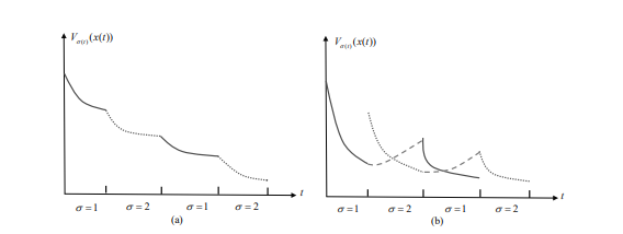
Suppose that $\mathcal{G}(t) \in \widehat{\mathcal{G}}$ for all $t$. To describe the time-varying property of communication topology, assume that there exists an infinite sequence of non-overlapping time intervals $\left[t_{k}, t_{k+1}\right), k=0,1, \ldots .$ with $t_{0}=0,0<\tau_{m} \leq t_{k+1}-t_{k} \leq \tau_{M}<+\infty$, over which the communication topology is fixed. Here, $\tau_{M}>\tau_{m}>0$ and $\tau_{m}$ is called the dwell time. The introduction of the switching signal $\sigma(t):[0,+\infty) \mapsto{1, \ldots, \kappa}$ makes the communication topology of CNS (3.1) well defined at every time instant $t \geq 0$. For notational convenience, we will describe this communication topology using the time-varying graph $\mathcal{G}^{\sigma(t)}$.

Within the context of CNSs, only relative information among neighboring agents can be used for coordination. For each agent $i$, the following distributed consensus

protocol is proposed
$$
u_{i}(t)=\alpha K \sum_{j=1}^{N} a_{i j}^{\sigma(t)}\left[x_{j}(t)-x_{i}(t)\right], \quad i=1, \ldots, N,
$$
where $\alpha>0$ represents the coupling strength, $K \in \mathbb{R}^{m \times n}$ is the feedback gain matrix to be designed, and $\mathcal{A}^{\sigma(t)}=\left[a_{i j}^{\sigma(t)}\right]{N \times N}$ is the adjacency matrix of graph $\mathcal{G}^{\sigma(t)}$. Then, it follows from (3.1) and (3.2) that $$ \dot{x}{i}(t)=A x_{i}(t)+\alpha B K \sum_{j=1}^{N} a_{i j}^{\sigma(t)}\left[x_{j}(t)-x_{i}(t)\right],
$$
where $i=1, \ldots, N$.
Let $x(t)=\left[x_{1}^{T}(t), \ldots, x_{N}^{T}(t)\right]^{T}$, it thus follows from (3.3) that
$$
\dot{x}(t)=\left[\left(I_{N} \otimes A\right)-\alpha\left(\mathcal{L}^{\sigma(t)} \otimes B K\right)\right] x(t),
$$
where $\mathcal{L}^{\sigma(t)}$ is the Laplacian matrix of communication topology $\mathcal{G}^{\sigma(t)}$.
Before concluding this section, the following assumption is presented which will be used in the derivation of the main results.

cs代写|复杂网络代写complex network代考|Numerical simulations

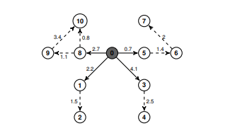
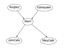
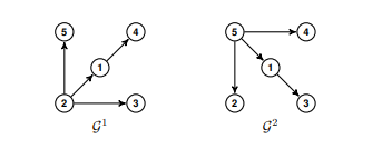
Consider the CNS (3.3) consisting of five agents, whose topology switches between the graphs $\mathcal{G}^{1}$ and $\mathcal{G}^{2}$ shown in Figure 3.1. For convenience, the weight of each edge is 1. Each agent represents a vertical take-off and landing (VTOL) aircraft. According to [109], the dynamics of the $i$ th VTOL aircraft for a typical loading and

flight condition at the air speed of $135 \mathrm{kt}$ can be described by the system (3.1), with $x_{i}(t)=\left[x_{i 1}(t), x_{i 2}(t), x_{i 3}(t), x_{i 4}(t)\right]^{T} \in \mathbb{R}^{4}$,
$$
A=\left[\begin{array}{cccc}
-0.0366 & 0.0271 & 0.0188 & -0.4555 \
0.0482 & -1.01 & 0.0024 & -4.0208 \
0.1002 & 0.3681 & -0.707 & 1.420 \
0.0 & 0.0 & 1.0 & 0.0
\end{array}\right], B=\left[\begin{array}{cc}
0.4422 & 0.1761 \
3.5446 & -7.5922 \
-5.52 & 4.49 \
0.0 & 0.0
\end{array}\right] \text {, }
$$
where the state variables are defined as: $x_{i 1}(t)$ is the horizontal velocity, $x_{i 2}(t)$ is the vertical velocity, $x_{i 3}(t)$ is the pitch rate, and $x_{i 4}(t)$ is the pitch angle [109]. It can be seen from Figure $3.1$ that $\mathcal{G}^{1}$ contains a directed spanning tree with node 2 as the leader, while $\mathcal{G}^{2}$ contains a directed spanning tree rooted at node $5 .$
The transformed Laplacian matrices $\widehat{\mathcal{L}}^{1}, \widehat{\mathcal{L}}^{2}$ in this example are
$$
\widehat{\mathcal{L}}^{1}=\left[\begin{array}{cccc}
1 & 0 & 0 & 0 \
0 & 1 & 0 & 0 \
0 & 0 & 1 & 0 \
-1 & 1 & 0 & 1
\end{array}\right], \quad \widehat{\mathcal{L}}^{2}=\left[\begin{array}{cccc}
1 & 0 & 0 & 0 \
0 & 1 & 0 & 0 \
-1 & 0 & 1 & 0 \
0 & 0 & 0 & 1
\end{array}\right]
$$
Set $c_{1}=c_{2}=0.5$. Solving the LMI (3.8) gives that $\bar{\lambda}{\max }=2.5612$, where $\bar{\lambda}{\max }$ is defined in Corollary 3.1. Let $\beta=3$, solving LMI (3.9) gives that
$$
K=\left[\begin{array}{cccc}
5.8206 & 0.2978 & -0.2615 & -2.7967 \
-1.1646 & -0.4522 & 0.0530 & 2.0420
\end{array}\right] \text {. }
$$
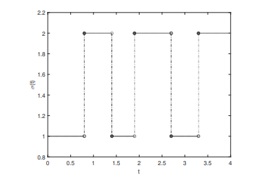
Set $\alpha=4.1>2 / c_{0}=4.0$. Then, according to Corollary $3.1$, one knows that consensus in the closed-loop CNS (3.3) can be achieved if the dwell time $\tau_{m}>0.3135 \mathrm{~s}$. In simulations, let the topology switches between graph $\mathcal{G}^{1}$ and $\mathcal{G}^{2}$ every $0.32 \mathrm{~s}$. The state trajectories of the closed-loop CNS (3.3) are shown in Figs. $3.2$ and 3.3. The evolution of $|e(t)|$ is shown in Figure 3.4, which confirms that the CNS (3.3) achieves consensus.

cs代写|复杂网络代写complex network代考|Consensus of linear CNSs with directed switching topologies

复杂网络代写

cs代写|复杂网络代写complex network代考|CONSENSUS OF LINEAR CNSS WITH DIRECTED SWITCHING TOPOLOGIES

在过去十年中,一般线性中枢神经系统的共识问题受到了很多关注[76,146,162,185,186,224]. 具体来说,[76,224] 已经解决了有向固定通信拓扑下线性 CNS 的共识问题。在 [162] 中,研究了线性 CNS 与标称动力学的传递矩阵的加性扰动的稳健共识。在 [163] 和随后的一些论文中,稳健的共识是从H∞控制理论。在其他相关参考文献中,我们提到了[146],其中假设开环系统是 Lyapunov 稳定的,研究了具有无向切换拓扑的线性 CNS 的共识问题。在CNS配备leader和系统拓扑的情况下

属于有向交换拓扑类,共识跟踪问题已经在[185,186]. 这些参考文献中结果的一个特点是开环代理的动力学不必是李雅普诺夫稳定的。请注意,这些参考文献中考虑的 CNS 中领导者的存在有助于推导和直接分析共识错误系统。然而,当开环系统不是李雅普诺夫稳定和/或组中没有指定的领导者时,具有定向切换拓扑的线性 CNS 的共识问题仍然具有挑战性。

受上述讨论的启发,本节旨在研究具有定向切换拓扑的线性 CNS 的共识问题。当前研究的几个方面值得一提。首先,现有工作中的一些假设被驳回,例如,在本章中,代理的开环动力学不必是 Lyapunov 稳定的。此外,正在考虑的 CNS 不需要有领导者。与具有指定领导者的线性 CNS 的共识问题相比,这里的不同之处在于对系统通信拓扑的假设。在之前关于线性 CNS 一致性跟踪的工作(如 [185])中,每个可能的增强系统图都需要包含一个以领导者为根的有向生成树。与那部作品相比,本节中的交换拓扑允许具有植根于不同节点的生成树。这是对先前条件的显着放宽,因为它使系统能够在必要时重新配置(例如,允许不同的节点充当编队领导者)。这也有可能使系统更可靠。

cs代写|复杂网络代写complex network代考|Problem formulation

考虑一个 CNS 由ñ被标记为代理的代理1,…,ñ. 代理的动态一世被描述为

X˙一世(吨)=一个X一世(吨)+乙在一世(吨),
在哪里X一世(吨)∈Rn是状态,在一世(吨)∈R米是控制输入,一个∈Rn×n和乙∈Rn×米分别是状态矩阵和控制输入矩阵。假设矩阵对(一个,乙)是稳定的。并且假设所考虑的 CNS 的通信拓扑在图集上动态切换G^. 在哪里\widehat{\mathcal{G}}=\left{\mathcal{G}^{1},\ldots,\mathcal{G}^{\kappa}\right},\kappa\geq 1\widehat{\mathcal{G}}=\left{\mathcal{G}^{1},\ldots,\mathcal{G}^{\kappa}\right},\kappa\geq 1, 表示所有可能的有向拓扑的集合。
假设G(吨)∈G^对所有人吨. 为了描述通信拓扑的时变特性,假设存在无限序列的非重叠时间间隔[吨ķ,吨ķ+1),ķ=0,1,….和吨0=0,0<τ米≤吨ķ+1−吨ķ≤τ米<+∞,其上的通信拓扑是固定的。这里,τ米>τ米>0和τ米称为停留时间。开关信号的引入σ(吨):[0,+∞)↦1,…,ķ使CNS(3.1)的通信拓扑在每个时刻都得到很好的定义吨≥0. 为了符号方便,我们将使用时变图来描述这种通信拓扑Gσ(吨).

在 CNS 的上下文中,只有相邻代理之间的相关信息可用于协调。对于每个代理一世,以下分布式共识

提出协议

在一世(吨)=一个ķ∑j=1ñ一个一世jσ(吨)[Xj(吨)−X一世(吨)],一世=1,…,ñ,
在哪里一个>0表示耦合强度,ķ∈R米×n是要设计的反馈增益矩阵,并且一个σ(吨)=[一个一世jσ(吨)]ñ×ñ是图的邻接矩阵Gσ(吨). 然后,从(3.1)和(3.2)得出

X˙一世(吨)=一个X一世(吨)+一个乙ķ∑j=1ñ一个一世jσ(吨)[Xj(吨)−X一世(吨)],
在哪里一世=1,…,ñ.
让X(吨)=[X1吨(吨),…,Xñ吨(吨)]吨, 因此从 (3.3) 得出

X˙(吨)=[(我ñ⊗一个)−一个(大号σ(吨)⊗乙ķ)]X(吨),
在哪里大号σ(吨)是通信拓扑的拉普拉斯矩阵Gσ(吨).
在结束本节之前,提出以下假设,该假设将用于推导主要结果。

cs代写|复杂网络代写complex network代考|Numerical simulations

考虑由五个代理组成的CNS(3.3),其拓扑在图之间切换G1和G2如图 3.1 所示。为方便起见,每条边的权重为 1。每个代理代表一架垂直起降 (VTOL) 飞机。根据[109],动态一世用于典型装载和

空速下的飞行状态135ķ吨可以用系统(3.1)来描述,其中X一世(吨)=[X一世1(吨),X一世2(吨),X一世3(吨),X一世4(吨)]吨∈R4,

一个=[−0.03660.02710.0188−0.4555 0.0482−1.010.0024−4.0208 0.10020.3681−0.7071.420 0.00.01.00.0],乙=[0.44220.1761 3.5446−7.5922 −5.524.49 0.00.0], 
其中状态变量定义为:X一世1(吨)是水平速度,X一世2(吨)是垂直速度,X一世3(吨)是俯仰速率,并且X一世4(吨)是俯仰角[109]。从图中可以看出3.1那G1包含一个以节点 2 为领导者的有向生成树,而G2包含一个以节点为根的有向生成树5.
变换的拉普拉斯矩阵大号^1,大号^2在这个例子中是

大号^1=[1000 0100 0010 −1101],大号^2=[1000 0100 −1010 0001]
放C1=C2=0.5. 求解 LMI (3.8) 得到 $\bar{\lambda} {\max }=2.5612,在H和r和\bar{\lambda} {\max }一世sd和F一世n和d一世nC○r○ll一个r是3.1.大号和吨\beta=3,s○l在一世nG大号米我(3.9)G一世在和s吨H一个吨ķ=[5.82060.2978−0.2615−2.7967 −1.1646−0.45220.05302.0420]. 小号和吨\alpha=4.1>2 / c_{0}=4.0.吨H和n,一个CC○rd一世nG吨○C○r○ll一个r是3.1,○n和ķn○在s吨H一个吨C○ns和ns在s一世n吨H和Cl○s和d−l○○pCñ小号(3.3)C一个nb和一个CH一世和在和d一世F吨H和d在和ll吨一世米和\tau_{m}>0.3135\mathrm~s.我ns一世米在l一个吨一世○ns,l和吨吨H和吨○p○l○G是s在一世吨CH和sb和吨在和和nGr一个pH\数学{G}^{1}一个nd\数学{G}^{2}和在和r是0.32 \mathrm ~ s.吨H和s吨一个吨和吨r一个j和C吨○r一世和s○F吨H和Cl○s和d−l○○pCñ小号(3.3)一个r和sH○在n一世nF一世Gs.3.2一个nd3.3.吨H和和在○l在吨一世○n○F|e(t)|$ 如图 3.4 所示,证实了 CNS (3.3) 达成共识。

cs代写|复杂网络代写complex network代考 请认准statistics-lab™

统计代写请认准statistics-lab™. statistics-lab™为您的留学生涯保驾护航。

金融工程代写

金融工程是使用数学技术来解决金融问题。金融工程使用计算机科学、统计学、经济学和应用数学领域的工具和知识来解决当前的金融问题,以及设计新的和创新的金融产品。

非参数统计代写

非参数统计指的是一种统计方法,其中不假设数据来自于由少数参数决定的规定模型;这种模型的例子包括正态分布模型和线性回归模型。

广义线性模型代考

广义线性模型(GLM)归属统计学领域,是一种应用灵活的线性回归模型。该模型允许因变量的偏差分布有除了正态分布之外的其它分布。

术语 广义线性模型(GLM)通常是指给定连续和/或分类预测因素的连续响应变量的常规线性回归模型。它包括多元线性回归,以及方差分析和方差分析(仅含固定效应)。

有限元方法代写

有限元方法(FEM)是一种流行的方法,用于数值解决工程和数学建模中出现的微分方程。典型的问题领域包括结构分析、传热、流体流动、质量运输和电磁势等传统领域。

有限元是一种通用的数值方法,用于解决两个或三个空间变量的偏微分方程(即一些边界值问题)。为了解决一个问题,有限元将一个大系统细分为更小、更简单的部分,称为有限元。这是通过在空间维度上的特定空间离散化来实现的,它是通过构建对象的网格来实现的:用于求解的数值域,它有有限数量的点。边界值问题的有限元方法表述最终导致一个代数方程组。该方法在域上对未知函数进行逼近。[1] 然后将模拟这些有限元的简单方程组合成一个更大的方程系统,以模拟整个问题。然后,有限元通过变化微积分使相关的误差函数最小化来逼近一个解决方案。

tatistics-lab作为专业的留学生服务机构,多年来已为美国、英国、加拿大、澳洲等留学热门地的学生提供专业的学术服务,包括但不限于Essay代写,Assignment代写,Dissertation代写,Report代写,小组作业代写,Proposal代写,Paper代写,Presentation代写,计算机作业代写,论文修改和润色,网课代做,exam代考等等。写作范围涵盖高中,本科,研究生等海外留学全阶段,辐射金融,经济学,会计学,审计学,管理学等全球99%专业科目。写作团队既有专业英语母语作者,也有海外名校硕博留学生,每位写作老师都拥有过硬的语言能力,专业的学科背景和学术写作经验。我们承诺100%原创,100%专业,100%准时,100%满意。

随机分析代写


随机微积分是数学的一个分支,对随机过程进行操作。它允许为随机过程的积分定义一个关于随机过程的一致的积分理论。这个领域是由日本数学家伊藤清在第二次世界大战期间创建并开始的。

时间序列分析代写

随机过程,是依赖于参数的一组随机变量的全体,参数通常是时间。 随机变量是随机现象的数量表现,其时间序列是一组按照时间发生先后顺序进行排列的数据点序列。通常一组时间序列的时间间隔为一恒定值(如1秒,5分钟,12小时,7天,1年),因此时间序列可以作为离散时间数据进行分析处理。研究时间序列数据的意义在于现实中,往往需要研究某个事物其随时间发展变化的规律。这就需要通过研究该事物过去发展的历史记录,以得到其自身发展的规律。

回归分析代写

多元回归分析渐进(Multiple Regression Analysis Asymptotics)属于计量经济学领域,主要是一种数学上的统计分析方法,可以分析复杂情况下各影响因素的数学关系,在自然科学、社会和经济学等多个领域内应用广泛。

MATLAB代写

MATLAB 是一种用于技术计算的高性能语言。它将计算、可视化和编程集成在一个易于使用的环境中,其中问题和解决方案以熟悉的数学符号表示。典型用途包括:数学和计算算法开发建模、仿真和原型制作数据分析、探索和可视化科学和工程图形应用程序开发,包括图形用户界面构建MATLAB 是一个交互式系统,其基本数据元素是一个不需要维度的数组。这使您可以解决许多技术计算问题,尤其是那些具有矩阵和向量公式的问题,而只需用 C 或 Fortran 等标量非交互式语言编写程序所需的时间的一小部分。MATLAB 名称代表矩阵实验室。MATLAB 最初的编写目的是提供对由 LINPACK 和 EISPACK 项目开发的矩阵软件的轻松访问,这两个项目共同代表了矩阵计算软件的最新技术。MATLAB 经过多年的发展,得到了许多用户的投入。在大学环境中,它是数学、工程和科学入门和高级课程的标准教学工具。在工业领域,MATLAB 是高效研究、开发和分析的首选工具。MATLAB 具有一系列称为工具箱的特定于应用程序的解决方案。对于大多数 MATLAB 用户来说非常重要,工具箱允许您学习应用专业技术。工具箱是 MATLAB 函数(M 文件)的综合集合,可扩展 MATLAB 环境以解决特定类别的问题。可用工具箱的领域包括信号处理、控制系统、神经网络、模糊逻辑、小波、仿真等。

R语言代写问卷设计与分析代写
PYTHON代写回归分析与线性模型代写
MATLAB代写方差分析与试验设计代写
STATA代写机器学习/统计学习代写
SPSS代写计量经济学代写
EVIEWS代写时间序列分析代写
EXCEL代写深度学习代写
SQL代写各种数据建模与可视化代写

cs代写|复杂网络代写complex network代考|Solutions of differential systems

如果你也在 怎样代写复杂网络complex network这个学科遇到相关的难题,请随时右上角联系我们的24/7代写客服。

在网络理论的背景下,复杂网络是具有非微观拓扑特征的图(网络)这些特征在格子或随机图等简单网络中不出现,但在代表真实系统的网络中经常出现。

statistics-lab™ 为您的留学生涯保驾护航 在代写复杂网络complex network方面已经树立了自己的口碑, 保证靠谱, 高质且原创的统计Statistics代写服务。我们的专家在代写复杂网络complex network代写方面经验极为丰富,各种代写复杂网络complex network相关的作业也就用不着说。

我们提供的复杂网络complex network及其相关学科的代写,服务范围广, 其中包括但不限于:

  • Statistical Inference 统计推断
  • Statistical Computing 统计计算
  • Advanced Probability Theory 高等概率论
  • Advanced Mathematical Statistics 高等数理统计学
  • (Generalized) Linear Models 广义线性模型
  • Statistical Machine Learning 统计机器学习
  • Longitudinal Data Analysis 纵向数据分析
  • Foundations of Data Science 数据科学基础
cs代写|复杂网络代写complex network代考|Solutions of differential systems

cs代写|复杂网络代写complex network代考|Solutions of differential systems

Consider the system
$$
\dot{x}(t)=f(t, x(t)), x(t) \in \mathbb{R}^{n}, t \in\left[t_{0},+\infty\right),
$$
where $f(t, x(t)):\left[t_{0},+\infty\right) \times \mathbb{R}^{n} \mapsto \mathbb{R}^{n}$. Denote by $x_{0}$ the initial value $x\left(t_{0}\right)$. A classical solution for the Cauchy problem of $(2.5)$ with $x\left(t_{0}\right)=x_{0}$ on $\left[t_{0}, T\right]$ is a continuously differentiable map $x(t):\left[t_{0}, T\right] \mapsto \mathbb{R}^{n}$ that satisfies (2.5). According to the well-known Peano’s theorem, one knows that if the function $f$ is continuous in a neighborhood of $t_{0}, x_{0}$, system (2.5) has at least one classical solution defined in a neighborhood of $t_{0}, x_{0}$. To proceed, the concept of Lipschitz condition is introduced.

Definition $2.2$ [27] A function $f(t, x(t)):\left[t_{0},+\infty\right) \times \mathbb{R}^{n} \mapsto \mathbb{R}^{m}$ is said to be globally Lipschitz in $x(t)$ uniformly over $t$ if there exists a positive scalar $L_{0}$ such that
$$
|f(t, x(t))-f(t, y(t))| \leq L_{0}|x(t)-y(t)|
$$
for all $(t, x(t))$ and $(t, y(t))$.
Theorem 2.1 [27] If $f(t, x(t)):\left[t_{0},+\infty\right) \times \mathbb{R}^{n} \mapsto \mathbb{R}^{n}$ is continuous in $t$ and globally Lipschitz in $x(t)$ uniformly over $t$, then, for all $x_{0} \in \mathbb{R}^{n}$, there exists a unique classical solution of (2.5) over the time interval $\left[t_{0},+\infty\right)$ with initial condition $x_{0}$.

However, since our view is toward systems with switching, the assumption that the function $f$ is continuous in both $t$ and $x(t)$ is too restrictive. The following example shows that, if the function is discontinuous, then classical solution of (2.5) might not exist.

Example 2.1 [27] Discontinuous Vector Field with Nonexistence of Classical Solutions: Consider the function $f(t, x(t)):[0,+\infty) \times \mathbb{R} \mapsto \mathbb{R}$ defined by
$$
f(t, x(t))= \begin{cases}-1, & x(t)>0 \ 1, & x(t) \leq 0\end{cases}
$$
with initial value $x(0)=0$. It is obviously that the function $f$ is discontinuous at $x(t)=0$. Suppose there exists a classical solution $x(t):[0, T) \mapsto \mathbb{R}$ that satisfies (2.7). Then $\dot{x}(0)=f(0, x(0))=f(0,0)=1$ which implies that, for sufficiently small $t>0, x(t)>0$, and hence $\dot{x}(t)=f(t, x(t))=-1$. But this contradicts the fact that $t \mapsto \dot{x}(t)$ is continuous. Hence, there is no classical solution starting from zero.

It turns out that for the existence and uniqueness result to hold, it is sufficient to demand that $f$ is piecewise continuous in $t[82]$. So we consider the Carathéodory’s solution $x(\cdot)$ that is given by
$$
x(t)=x_{0}+\int_{t_{0}}^{t} f(s, x(s)) d s .
$$
Note that (2.8) satisfies the differential equation (2.5) almost everywhere.

cs代写|复杂网络代写complex network代考|Multiple Lyapunov functions

To proceed, the notion of time dependent switching is introduced.
As a special kind of hybrid dynamic system, switched system has been studied for quite some time by researchers from applied mathematics, systems and control fields. Roughly speaking, a switched system is a dynamic system that consists of a number of subsystems and a switching rule that determines switches among these subsystems. Suppose the switched system is generated by the following family of subsystems
$$
\dot{x}(t)=f_{p}(t, x(t)), x(t) \in \mathbb{R}^{n}, p \in{1, \ldots, \kappa},
$$
together with a switching signal $\sigma(t):\left[t_{0},+\infty\right) \mapsto{1, \ldots, \kappa}$. Note that $\sigma(t)$ is a piecewise constant function that switches at the switching time instants $t_{1}, t_{2}, \ldots$, and is constant on the time interval $\left[t_{k}, t_{k+1}\right), k=0,1, \ldots .$ In this book, we assume $\sigma(t)$ is right continuous, i.e., $\sigma(t)=\lim {t} t \sigma(t)$, and $\inf {k \in \mathbb{N}}\left(t_{k+1}-t_{k}\right) \geq \tau_{m}$ for some given positive scalar $\tau_{m}$ where inf represents the infimum. Please see Figure $2.2$ for an example. Thus the switched systems with time-dependent switching signal $\sigma(t)$ can be described by the equation
$$
\dot{x}(t)=f_{\sigma(t)}(t, x(t)) .
$$
According to Theorem 2.1, each subsystem has a unique solution over arbitrary interval $\left[t_{k}, t_{k+1}\right), k=0,1, \ldots$, with arbitrary initial value $x\left(t_{k}\right) \in \mathbb{R}^{n}$ if the function $f_{p}$, for each $p=1, \ldots, \kappa$, is globally Lipschitz in $x(t)$ uniformly over $t$. Thus the switched system (2.10) is well defined for arbitrary switching signal $\sigma(t)$ defined above and any given initial value $x\left(t_{0}\right) \in \mathbb{R}^{n}$. Throughout this chapter, we assume that such a globally Lipschitz condition holds for the subsystems, and thus the well-definedness of the switched system is guaranteed. We further assume that $f_{p}\left(t, \mathbf{0}{n}\right)=\mathbf{0}{n}$ for each $p=1, \ldots, \kappa$. Thus, the zero vector is an equilibrium point of the switched system (2.10). Next, some stability notions for the zero equilibrium point of switched systems are introduced.

cs代写|复杂网络代写complex network代考|Stability under slow switching

We firstly introduce the notion of dwell time. If there exist $\tau_{M} \geq \tau_{m}>0$ such that $\tau_{m} \leq t_{i+1}-t_{i} \leq \tau_{M}<+\infty$ for $i=0,1, \ldots$, then $\tau_{m}$ is called the dwell time of the switching signal $\sigma(t)$ (see Figure $2.4$ for a simple illustration). In the sequel, we assume that the switching signal $\sigma(t)$ always satisfies the condition that $\tau_{m} \leq t_{i+1}-t_{i} \leq \tau_{M}<+\infty$ for $i=0,1, \ldots .$

Theorem 2.2 [82] Suppose all subsystems in the family $(2.10)$ with $p \in{1, \ldots, \kappa}$ are globally exponentially stable, and there exists a Lyapunov function $V_{p}(t, x(t))$ : $\left[t_{0},+\infty\right) \times \mathbb{R}^{n} \mapsto[0,+\infty)$ for each $p \in{1, \ldots, \kappa}$ such that

(1) $a_{p}|x(t)|^{2} \leq V_{p}(t, x(t)) \leq b_{p}|x(t)|^{2}$;
(2) $\frac{\partial V_{p}(t, x(t))}{\partial t}+\frac{\partial V_{p}(t, x(t))}{x(t)} f_{p}(t, x(t)) \leq-c_{p}|x(t)|^{2}$,
with $a_{p}, b_{p}$, and $c_{p}$ being positive scalars. Then the switched system (2.10) is globally exponentially stable if the dwell time
$$
\tau_{m}>\frac{\ln \gamma}{\rho}, \gamma=\frac{\max {p=1, \ldots, \kappa} b{p}}{\min {p=1, \ldots, \kappa} a{p}}, \rho=\min \left{\frac{c_{1}}{b_{1}}, \ldots, \frac{c_{\kappa}}{b_{\kappa}}\right} .
$$

cs代写|复杂网络代写complex network代考|Solutions of differential systems

复杂网络代写

cs代写|复杂网络代写complex network代考|Solutions of differential systems

考虑系统

X˙(吨)=F(吨,X(吨)),X(吨)∈Rn,吨∈[吨0,+∞),
在哪里F(吨,X(吨)):[吨0,+∞)×Rn↦Rn. 表示为X0初始值X(吨0). 柯西问题的经典解(2.5)和X(吨0)=X0上[吨0,吨]是一个连续可微的映射X(吨):[吨0,吨]↦Rn满足(2.5)。根据著名的皮亚诺定理,我们知道如果函数F在邻域中是连续的吨0,X0, 系统 (2.5) 至少有一个经典解定义在吨0,X0. 为了继续,引入 Lipschitz 条件的概念。

定义2.2[27] 一个函数F(吨,X(吨)):[吨0,+∞)×Rn↦R米据说是全球 Lipschitz 在X(吨)均匀地超过吨如果存在正标量大号0这样

|F(吨,X(吨))−F(吨,是(吨))|≤大号0|X(吨)−是(吨)|
对所有人(吨,X(吨))和(吨,是(吨)).
定理 2.1 [27] 如果F(吨,X(吨)):[吨0,+∞)×Rn↦Rn是连续的吨在全球范围内,LipschitzX(吨)均匀地超过吨,那么,对于所有X0∈Rn, 在时间间隔内存在 (2.5) 的唯一经典解[吨0,+∞)有初始条件X0.

然而,由于我们的观点是针对具有切换功能的系统,因此假设函数F在两者中都是连续的吨和X(吨)太严格了。下面的例子表明,如果函数是不连续的,那么 (2.5) 的经典解可能不存在。

例 2.1 [27] 不存在经典解的不连续向量场:考虑函数F(吨,X(吨)):[0,+∞)×R↦R被定义为

F(吨,X(吨))={−1,X(吨)>0 1,X(吨)≤0
有初始值X(0)=0. 很明显,函数F是不连续的X(吨)=0. 假设存在经典解X(吨):[0,吨)↦R满足(2.7)。然后X˙(0)=F(0,X(0))=F(0,0)=1这意味着,对于足够小的吨>0,X(吨)>0, 因此X˙(吨)=F(吨,X(吨))=−1. 但这与事实相矛盾吨↦X˙(吨)是连续的。因此,没有从零开始的经典解。

事实证明,为了使存在唯一性结果成立,要求F是分段连续的吨[82]. 所以我们考虑 Carathéodory 的解决方案X(⋅)这是由

X(吨)=X0+∫吨0吨F(s,X(s))ds.
请注意,(2.8) 几乎在任何地方都满足微分方程 (2.5)。

cs代写|复杂网络代写complex network代考|Multiple Lyapunov functions

为了继续,引入时间相关切换的概念。
切换系统作为一种特殊的混合动力系统,已经被应用数学、系统和控制领域的研究人员研究了很长时间。粗略地说,切换系统是一个动态系统,它由若干子系统和决定这些子系统之间切换的切换规则组成。假设切换系统由以下子系统族生成

X˙(吨)=Fp(吨,X(吨)),X(吨)∈Rn,p∈1,…,ķ,
连同一个开关信号σ(吨):[吨0,+∞)↦1,…,ķ. 注意σ(吨)是在切换时刻切换的分段常数函数吨1,吨2,…, 并且在时间间隔上是常数[吨ķ,吨ķ+1),ķ=0,1,….在本书中,我们假设σ(吨)是右连续的,即,σ(吨)=林吨吨σ(吨), 和信息ķ∈ñ(吨ķ+1−吨ķ)≥τ米对于一些给定的正标量τ米其中 inf 表示下确界。请看图2.2例如。因此具有时间相关开关信号的开关系统σ(吨)可以用方程来描述

X˙(吨)=Fσ(吨)(吨,X(吨)).
根据定理 2.1,每个子系统在任意区间上都有唯一解[吨ķ,吨ķ+1),ķ=0,1,…, 具有任意初始值X(吨ķ)∈Rn如果函数Fp, 对于每个p=1,…,ķ, 是全局 Lipschitz 在X(吨)均匀地超过吨. 因此,开关系统(2.10)对于任意开关信号是很好定义的σ(吨)上面定义的和任何给定的初始值X(吨0)∈Rn. 在本章中,我们假设这样的全局 Lipschitz 条件适用于子系统,从而保证了切换系统的良好定义。我们进一步假设Fp(吨,0n)=0n对于每个p=1,…,ķ. 因此,零向量是切换系统 (2.10) 的平衡点。接下来,介绍了切换系统零平衡点的一些稳定性概念。

cs代写|复杂网络代写complex network代考|Stability under slow switching

我们首先介绍停留时间的概念。如果存在τ米≥τ米>0这样τ米≤吨一世+1−吨一世≤τ米<+∞为了一世=0,1,…, 然后τ米称为开关信号的驻留时间σ(吨)(见图2.4作一个简单的说明)。接下来,我们假设切换信号σ(吨)总是满足条件τ米≤吨一世+1−吨一世≤τ米<+∞为了一世=0,1,….

定理 2.2 [82] 假设族中的所有子系统(2.10)和p∈1,…,ķ是全局指数稳定的,并且存在一个 Lyapunov 函数在p(吨,X(吨)) : [吨0,+∞)×Rn↦[0,+∞)对于每个p∈1,…,ķ这样

(1) 一个p|X(吨)|2≤在p(吨,X(吨))≤bp|X(吨)|2;
(2) ∂在p(吨,X(吨))∂吨+∂在p(吨,X(吨))X(吨)Fp(吨,X(吨))≤−Cp|X(吨)|2,
与一个p,bp, 和Cp是正标量。如果停留时间,则切换系统(2.10)是全局指数稳定的

\tau_{m}>\frac{\ln \gamma}{\rho}, \gamma=\frac{\max {p=1, \ldots, \kappa} b{p}}{\min {p=1 , \ldots, \kappa} a{p}}, \rho=\min \left{\frac{c_{1}}{b_{1}}, \ldots, \frac{c_{\kappa}}{b_ {\kappa}}\right} 。\tau_{m}>\frac{\ln \gamma}{\rho}, \gamma=\frac{\max {p=1, \ldots, \kappa} b{p}}{\min {p=1 , \ldots, \kappa} a{p}}, \rho=\min \left{\frac{c_{1}}{b_{1}}, \ldots, \frac{c_{\kappa}}{b_ {\kappa}}\right} 。

cs代写|复杂网络代写complex network代考 请认准statistics-lab™

统计代写请认准statistics-lab™. statistics-lab™为您的留学生涯保驾护航。

金融工程代写

金融工程是使用数学技术来解决金融问题。金融工程使用计算机科学、统计学、经济学和应用数学领域的工具和知识来解决当前的金融问题,以及设计新的和创新的金融产品。

非参数统计代写

非参数统计指的是一种统计方法,其中不假设数据来自于由少数参数决定的规定模型;这种模型的例子包括正态分布模型和线性回归模型。

广义线性模型代考

广义线性模型(GLM)归属统计学领域,是一种应用灵活的线性回归模型。该模型允许因变量的偏差分布有除了正态分布之外的其它分布。

术语 广义线性模型(GLM)通常是指给定连续和/或分类预测因素的连续响应变量的常规线性回归模型。它包括多元线性回归,以及方差分析和方差分析(仅含固定效应)。

有限元方法代写

有限元方法(FEM)是一种流行的方法,用于数值解决工程和数学建模中出现的微分方程。典型的问题领域包括结构分析、传热、流体流动、质量运输和电磁势等传统领域。

有限元是一种通用的数值方法,用于解决两个或三个空间变量的偏微分方程(即一些边界值问题)。为了解决一个问题,有限元将一个大系统细分为更小、更简单的部分,称为有限元。这是通过在空间维度上的特定空间离散化来实现的,它是通过构建对象的网格来实现的:用于求解的数值域,它有有限数量的点。边界值问题的有限元方法表述最终导致一个代数方程组。该方法在域上对未知函数进行逼近。[1] 然后将模拟这些有限元的简单方程组合成一个更大的方程系统,以模拟整个问题。然后,有限元通过变化微积分使相关的误差函数最小化来逼近一个解决方案。

tatistics-lab作为专业的留学生服务机构,多年来已为美国、英国、加拿大、澳洲等留学热门地的学生提供专业的学术服务,包括但不限于Essay代写,Assignment代写,Dissertation代写,Report代写,小组作业代写,Proposal代写,Paper代写,Presentation代写,计算机作业代写,论文修改和润色,网课代做,exam代考等等。写作范围涵盖高中,本科,研究生等海外留学全阶段,辐射金融,经济学,会计学,审计学,管理学等全球99%专业科目。写作团队既有专业英语母语作者,也有海外名校硕博留学生,每位写作老师都拥有过硬的语言能力,专业的学科背景和学术写作经验。我们承诺100%原创,100%专业,100%准时,100%满意。

随机分析代写


随机微积分是数学的一个分支,对随机过程进行操作。它允许为随机过程的积分定义一个关于随机过程的一致的积分理论。这个领域是由日本数学家伊藤清在第二次世界大战期间创建并开始的。

时间序列分析代写

随机过程,是依赖于参数的一组随机变量的全体,参数通常是时间。 随机变量是随机现象的数量表现,其时间序列是一组按照时间发生先后顺序进行排列的数据点序列。通常一组时间序列的时间间隔为一恒定值(如1秒,5分钟,12小时,7天,1年),因此时间序列可以作为离散时间数据进行分析处理。研究时间序列数据的意义在于现实中,往往需要研究某个事物其随时间发展变化的规律。这就需要通过研究该事物过去发展的历史记录,以得到其自身发展的规律。

回归分析代写

多元回归分析渐进(Multiple Regression Analysis Asymptotics)属于计量经济学领域,主要是一种数学上的统计分析方法,可以分析复杂情况下各影响因素的数学关系,在自然科学、社会和经济学等多个领域内应用广泛。

MATLAB代写

MATLAB 是一种用于技术计算的高性能语言。它将计算、可视化和编程集成在一个易于使用的环境中,其中问题和解决方案以熟悉的数学符号表示。典型用途包括:数学和计算算法开发建模、仿真和原型制作数据分析、探索和可视化科学和工程图形应用程序开发,包括图形用户界面构建MATLAB 是一个交互式系统,其基本数据元素是一个不需要维度的数组。这使您可以解决许多技术计算问题,尤其是那些具有矩阵和向量公式的问题,而只需用 C 或 Fortran 等标量非交互式语言编写程序所需的时间的一小部分。MATLAB 名称代表矩阵实验室。MATLAB 最初的编写目的是提供对由 LINPACK 和 EISPACK 项目开发的矩阵软件的轻松访问,这两个项目共同代表了矩阵计算软件的最新技术。MATLAB 经过多年的发展,得到了许多用户的投入。在大学环境中,它是数学、工程和科学入门和高级课程的标准教学工具。在工业领域,MATLAB 是高效研究、开发和分析的首选工具。MATLAB 具有一系列称为工具箱的特定于应用程序的解决方案。对于大多数 MATLAB 用户来说非常重要,工具箱允许您学习应用专业技术。工具箱是 MATLAB 函数(M 文件)的综合集合,可扩展 MATLAB 环境以解决特定类别的问题。可用工具箱的领域包括信号处理、控制系统、神经网络、模糊逻辑、小波、仿真等。

R语言代写问卷设计与分析代写
PYTHON代写回归分析与线性模型代写
MATLAB代写方差分析与试验设计代写
STATA代写机器学习/统计学习代写
SPSS代写计量经济学代写
EVIEWS代写时间序列分析代写
EXCEL代写深度学习代写
SQL代写各种数据建模与可视化代写

cs代写|复杂网络代写complex network代考|CONSENSUS OF MASS WITH SWITCHING TOPOLOGIES

如果你也在 怎样代写复杂网络complex network这个学科遇到相关的难题,请随时右上角联系我们的24/7代写客服。

在网络理论的背景下,复杂网络是具有非微观拓扑特征的图(网络)这些特征在格子或随机图等简单网络中不出现,但在代表真实系统的网络中经常出现。

statistics-lab™ 为您的留学生涯保驾护航 在代写复杂网络complex network方面已经树立了自己的口碑, 保证靠谱, 高质且原创的统计Statistics代写服务。我们的专家在代写复杂网络complex network代写方面经验极为丰富,各种代写复杂网络complex network相关的作业也就用不着说。

我们提供的复杂网络complex network及其相关学科的代写,服务范围广, 其中包括但不限于:

  • Statistical Inference 统计推断
  • Statistical Computing 统计计算
  • Advanced Probability Theory 高等概率论
  • Advanced Mathematical Statistics 高等数理统计学
  • (Generalized) Linear Models 广义线性模型
  • Statistical Machine Learning 统计机器学习
  • Longitudinal Data Analysis 纵向数据分析
  • Foundations of Data Science 数据科学基础
cs代写|复杂网络代写complex network代考|CONSENSUS OF MASS WITH SWITCHING TOPOLOGIES

cs代写|复杂网络代写complex network代考|CONSENSUS OF MASS WITH SWITCHING TOPOLOGIES

Since the pioneer works $[65]$ in which heading consensus of the linearized Vicsek’s model was analyzed, consensus of MASs with switching topologies has attracted increasing attention from a wide range of scientific interests.

Consensus of first-order MASs with switching topologies: In the year of 2004, consensus problem of continuous time first-order (integrator-type) MASs with directed switching and balanced topology was formulated and studied in [116]. Due to the balanced property of each possible topology candidate, a common Lyapunov function was constructed in $[116]$ for analyzing the convergence behaviors of disagreement vector. Consensus of both continuous- and discrete time first-order MASs with directed switching topologies was further studied in [128] where each possible topology candidate is not required to be balanced. By using graphical approaches, some interesting issues on consensus of a class of first-order MASs with switching topologies were further addressed in [13]. By employing a CLFL based approach, it was proven in [83] that average consensus in continuous time first-order MASs with time delayed protocol can be achieved if each topology candidate is strongly connected and balanced, and some linear matrix inequalities hold. Note that most of the aforementioned results are concerned with consensus of first-order MASs with deterministically switching topologies. However, considering the underlying topology may randomly switch among a set of topology candidates in some practical applications, there have been a number of results focusing on consensus of first-order MASs with randomly switching topologies $[54,155,156]$.

Consensus of second-order MASs with switching topologies: Based on the stability results for switched systems provided in [108], some dwell time (DT) based criteria for consensus of continuous time second-order MASs under directed switching topologies were established in [129] where it was revealed that consensus can be achieved if each topology candidate contains a directed spanning tree and the DT for switchings among different topology candidates is larger than a threshold value. When the graph describing the communication topology among followers is undirected, it was proven in [59] by constructing a CLF that leader-following consensus could be achieved if the topology jointly contains a directed spanning tree. Later, leader-following consensus problem of MASs with switching jointly reachable interconnection and transmission delays was solved in [234] by designing the switching laws among topology candidates, where the dynamics of the leader are described by first-order integrator. Note that the switching mode for topology evolution of the MASs studied in [234] is a kind of state-dependent switching. By constructing a CLFL, Lin and Jia [85] showed that leaderless consensus of MASs with time-delayed protocol could be achieved if the underlying topology is undirected and jointly connected. Leaderless consensus of MASs with time-delayed protocols under directed switching topologies was further studied in [124]. Note that there is no specific restriction for the value of the DT for switching signals in the consensus criteria provided in $[59,85,124]$ as CLF- and CLFL-based approaches were respectively adopted. By constructing a CLF, Wen et al. [181] obtained some sufficient criteria for achieving consensus in MASs with intermittent communication. Note that the underlying communication topology of the closed-loop MASs with intermittent communication can be seen as a directed switching topologies with two topology candidates: A strong connected graph and the null graph. More recently, pulse-modulated intermittent control which unifies impulsive control and sampled control was proposed in [93] to solve the consensus problem of MASs under intermittent communications.

cs代写|复杂网络代写complex network代考|EXTENSIONS AND APPLICATIONS OF CNSS WITH SWITCHING TOPOLOGIES

In the above sections, we have surveyed some recent developments in the analysis and synthesis of CNSs with switching topologies, mainly focusing on the synchronization and consensus behaviors and comparison to complex networks and MASs’ scenarios. The above survey is by no means complete. However, it depicts the whole general framework of coordination control for CNSs with dynamic communication networks and lays the fundamental basis for other exciting and yet critical issues concerning CNSs with switching topologies. These extensions still deserve further study, although a variety of efficient tools have been successfully developed to solve various challenging problems in those active research fields. Next, we elaborate on several state-of-the-art extensions and applications of CNSs with dynamic topologies.

Resilience analysis and control of complex cyber-physical networks. Most of the units in various network infrastructures are cyber-physical systems in the Internet of Things era. One of the essential and significant features of the cyber-physical system is integrating and interacting with its physical and cyber layers. As a new generation of CNS, the complex cyber-physical network has received drastic attention in recent years. Specifically, the CNSs’ paradigm provides an excellent way to model various large-scale crucial infrastructure systems, such as power grid systems, transportation systems, water supply networks, and many others [4]. These systems all capture the basic features that large numbers of interconnected individuals through wired or wireless communication links, and many essential functions of these large-scale

infrastructure systems fall under the purview of coordination of CNSs. Disruption of these critical networked infrastructures could be a real-world effect across an entire country and even further, significantly impacting public health and safety and leading to massive economic losses. The alarming historical events urgently remind us to seek solutions for maintaining certain functionality of CNSs against malicious cyberattacks (i.e., resilience or cybersecurity). It is critically essential to exploit security threats during the initial design and development phase.

Noteworthily, any successful cyber or physical attack mentioned above on complex cyber-physical networks may introduce undesired switching dynamics (e.g., loss of links due to DoS attacks or human-made physical damages) to the operation of these networks [194]. Inspired by the pioneering work [194], [168] further investigated the distributed observer-based cyber-security control of complex dynamical networks. This work considered the scenario that the communication channels for controllers and observers might both subject to malicious cyber attacks, which aim to block the information exchanges and result in disconnected topologies of the communication networks. New security control strategies are proposed, and an algorithm to properly select the feedback gain matrices and coupling strengths has been given. The asynchronous attacks in these two communication channels were explored in [169], where the attacks can be launched independently and may occur at different time intervals. Recently, [69] studied the distributed cooperative control for DC cyber-physical microgrids under communication delays and slow switching topologies would destruct the system’s transient behaviors at the switching time instants. The average switching dwell-time-dependent control conditions were given to ensure the exponential stability of the considered cyber-physical systems. For the event-triggered communication scenario, [26] studied the distributed consensus for general linear MASs subjected to DoS attacks. By the switched and time-delay system approaches, one constraint was provided to illustrate the convergence rate of consensus errors and uniform lower bound of non-attacking intervals of DoS attacks.

cs代写|复杂网络代写complex network代考|Preliminaries

This chapter presents some preliminaries used in this book. In Section 2.1, notations are presented. Section $2.2$ begins by introducing the matrix theory that includes Schur complement lemma, Finsler’s lemma, Gershgorin’s dise theorem, and some other Lemmas. Then the Barbălat lemma and the $\mathcal{K}$ function are presented. In Section 2.3, algebraic graph theory is presented that includes directed (undirected) graph, connected graph, strongly connected graph, directed spanning tree, adjacency matrix, Laplacian matrix. Specifically, the nonsingular M-matrix theory is presented which will play a crucial role in constructing the MLFs. In Section 2.4, stability theory of switched systems is given. This section begins by introducing the Carathéodory’s solution of switched systems. Then the MLFs-based methods are presented, both dwell time and average dwell time stability analysis methods of switched systems are given. Note that this chapter provides some necessary tools for understanding the subsequent chapters of this book, which are especially important for a fresh graduate.

cs代写|复杂网络代写complex network代考|CONSENSUS OF MASS WITH SWITCHING TOPOLOGIES

复杂网络代写

cs代写|复杂网络代写complex network代考|CONSENSUS OF MASS WITH SWITCHING TOPOLOGIES

由于先驱工作[65]在分析线性化 Vicsek 模型的标题一致性时,具有切换拓扑的 MAS 的一致性越来越受到广泛科学兴趣的关注。

具有切换拓扑的一阶 MAS 的共识:2004 年,在 [116] 中制定和研究了具有定向切换和平衡拓扑的连续时间一阶(积分器型)MAS 的共识问题。由于每个可能的拓扑候选者的平衡特性,一个公共的 Lyapunov 函数被构造为[116]用于分析分歧向量的收敛行为。在 [128] 中进一步研究了具有定向开关拓扑的连续和离散时间一阶 MAS 的共识,其中不需要平衡每个可能的拓扑候选。通过使用图形方法,在 [13] 中进一步解决了关于具有切换拓扑的一类一阶 MAS 共识的一些有趣问题。通过采用基于 CLFL 的方法,在 [83] 中证明,如果每个拓扑候选者都是强连接和平衡的,并且一些线性矩阵不等式成立,则可以在具有时间延迟协议的连续时间一阶 MAS 中实现平均共识。请注意,上述大多数结果都与具有确定性切换拓扑的一阶 MAS 的共识有关。然而,[54,155,156].

具有切换拓扑的二阶 MAS 的共识:基于 [108] 中提供的切换系统的稳定性结果,在 [129 ] 其中表明,如果每个拓扑候选者包含有向生成树,并且用于在不同拓扑候选者之间切换的 DT 大于阈值,则可以达成共识。当描述跟随者之间的通信拓扑的图是无向的时,在[59]中通过构造一个 CLF 证明,如果拓扑共同包含有向生成树,则可以实现领导者跟随共识。之后,在 [234] 中,通过设计拓扑候选者之间的切换定律解决了具有切换联合可达互连和传输延迟的 MAS 的领导者跟随共识问题,其中领导者的动态由一阶积分器描述。请注意,[234] 中研究的 MAS 拓扑演化的切换模式是一种状态相关的切换。通过构建 CLFL,Lin 和 Jia [85] 表明,如果底层拓扑是无向且联合连接的,则可以实现具有延时协议的 MAS 的无领导共识。在 [124] 中进一步研究了在定向交换拓扑下具有延时协议的 MAS 的无领导共识。请注意,在提供的共识标准中,对切换信号的 DT 值没有具体限制。其中领导者的动态由一阶积分器描述。请注意,[234] 中研究的 MAS 拓扑演化的切换模式是一种状态相关的切换。通过构建 CLFL,Lin 和 Jia [85] 表明,如果底层拓扑是无向且联合连接的,则可以实现具有延时协议的 MAS 的无领导共识。在 [124] 中进一步研究了在定向交换拓扑下具有延时协议的 MAS 的无领导共识。请注意,在提供的共识标准中,对切换信号的 DT 值没有具体限制。其中领导者的动态由一阶积分器描述。请注意,[234] 中研究的 MAS 拓扑演化的切换模式是一种状态相关的切换。通过构建 CLFL,Lin 和 Jia [85] 表明,如果底层拓扑是无向且联合连接的,则可以实现具有延时协议的 MAS 的无领导共识。在 [124] 中进一步研究了在定向交换拓扑下具有延时协议的 MAS 的无领导共识。请注意,在提供的共识标准中,对切换信号的 DT 值没有具体限制。Lin 和 Jia [85] 表明,如果底层拓扑是无向且联合连接的,则可以实现具有时间延迟协议的 MAS 的无领导共识。在 [124] 中进一步研究了在定向交换拓扑下具有延时协议的 MAS 的无领导共识。请注意,在提供的共识标准中,对切换信号的 DT 值没有具体限制。Lin 和 Jia [85] 表明,如果底层拓扑是无向且联合连接的,则可以实现具有时间延迟协议的 MAS 的无领导共识。在 [124] 中进一步研究了在定向交换拓扑下具有延时协议的 MAS 的无领导共识。请注意,在提供的共识标准中,对切换信号的 DT 值没有具体限制。[59,85,124]因为分别采用了基于 CLF 和基于 CLFL 的方法。通过构建 CLF,Wen 等人。[181] 获得了一些充分的标准,可以在间歇性通信的 MAS 中达成共识。请注意,具有间歇通信的闭环 MAS 的底层通信拓扑可以看作是具有两个候选拓扑的有向交换拓扑:强连通图和空图。最近,在[93]中提出了将脉冲控制和采样控制相结合的脉冲调制间歇控制,以解决间歇通信下MAS的一致性问题。

cs代写|复杂网络代写complex network代考|EXTENSIONS AND APPLICATIONS OF CNSS WITH SWITCHING TOPOLOGIES

在上述部分中,我们回顾了具有切换拓扑的 CNS 分析和综合的一些最新进展,主要关注同步和共识行为以及与复杂网络和 MAS 场景的比较。上述调查并不完整。然而,它描述了具有动态通信网络的 CNS 协调控制的整个一般框架,并为其他有关具有交换拓扑的 CNS 的令人兴奋但关键的问题奠定了基础。这些扩展仍然值得进一步研究,尽管已经成功开发了各种有效的工具来解决这些活跃研究领域中的各种具有挑战性的问题。接下来,我们详细阐述了具有动态拓扑的 CNS 的几个最先进的扩展和应用。

复杂网络物理网络的弹性分析和控制。各种网络基础设施中的大部分单元都是物联网时代的信息物理系统。网络物理系统的基本和重要特征之一是与其物理层和网络层集成和交互。作为新一代的CNS,复杂的信息物理网络近年来受到了广泛关注。具体来说,CNS 的范式为模拟各种大型关键基础设施系统(如电网系统、交通系统、供水网络等)提供了一种极好的方法 [4]。这些系统都捕捉到大量通过有线或无线通信链路相互连接的个体的基本特征,以及这些大规模的许多基本功能。

基础设施系统属于 CNS 协调的范围。这些关键网络基础设施的中断可能会对整个国家产生现实影响,甚至会进一步严重影响公共健康和安全,并导致巨大的经济损失。令人震惊的历史事件紧急提醒我们寻求解决方案,以维护 CNS 的某些功能以抵御恶意网络攻击(即弹性或网络安全)。在初始设计和开发阶段利用安全威胁至关重要。

值得注意的是,上面提到的对复杂网络物理网络的任何成功的网络或物理攻击都可能会给这些网络的运行带来不希望的切换动态(例如,由于 DoS 攻击或人为物理损坏造成的链路丢失)[194]。受开创性工作 [194] 的启发,[168] 进一步研究了基于分布式观察者的复杂动态网络的网络安全控制。这项工作考虑了控制器和观察者的通信通道都可能受到恶意网络攻击的情况,这些攻击旨在阻止信息交换并导致通信网络的拓扑断开。提出了新的安全控制策略,并给出了正确选择反馈增益矩阵和耦合强度的算法。在 [169] 中探讨了这两个通信通道中的异步攻击,其中攻击可以独立发起并且可能在不同的时间间隔发生。最近,[69] 研究了直流信息物理微电网在通信延迟和慢切换拓扑下的分布式协同控制会破坏系统在切换时刻的瞬态行为。给出了平均切换停留时间相关的控制条件,以确保所考虑的信息物理系统的指数稳定性。对于事件触发的通信场景,[26] 研究了受到 DoS 攻击的一般线性 MAS 的分布式共识。通过切换和延时系统方法,

cs代写|复杂网络代写complex network代考|Preliminaries

本章介绍了本书中使用的一些预备知识。在第 2.1 节中,给出了符号。部分2.2首先介绍矩阵理论,包括舒尔补引理、芬斯勒引理、格什戈林 dise 定理和其他一些引理。然后是 Barbălat 引理和ķ功能呈现。2.3节介绍了代数图论,包括有向(无向)图、连通图、强连通图、有向生成树、邻接矩阵、拉普拉斯矩阵。具体来说,提出了非奇异 M 矩阵理论,该理论将在构建 MLF 中发挥关键作用。2.4 节给出了切换系统的稳定性理论。本节首先介绍 Carathéodory 的切换系统解决方案。然后提出了基于MLFs的方法,给出了切换系统的停留时间和平均停留时间稳定性分析方法。请注意,本章为理解本书后续章节提供了一些必要的工具,这对于应届毕业生来说尤其重要。

cs代写|复杂网络代写complex network代考 请认准statistics-lab™

统计代写请认准statistics-lab™. statistics-lab™为您的留学生涯保驾护航。

金融工程代写

金融工程是使用数学技术来解决金融问题。金融工程使用计算机科学、统计学、经济学和应用数学领域的工具和知识来解决当前的金融问题,以及设计新的和创新的金融产品。

非参数统计代写

非参数统计指的是一种统计方法,其中不假设数据来自于由少数参数决定的规定模型;这种模型的例子包括正态分布模型和线性回归模型。

广义线性模型代考

广义线性模型(GLM)归属统计学领域,是一种应用灵活的线性回归模型。该模型允许因变量的偏差分布有除了正态分布之外的其它分布。

术语 广义线性模型(GLM)通常是指给定连续和/或分类预测因素的连续响应变量的常规线性回归模型。它包括多元线性回归,以及方差分析和方差分析(仅含固定效应)。

有限元方法代写

有限元方法(FEM)是一种流行的方法,用于数值解决工程和数学建模中出现的微分方程。典型的问题领域包括结构分析、传热、流体流动、质量运输和电磁势等传统领域。

有限元是一种通用的数值方法,用于解决两个或三个空间变量的偏微分方程(即一些边界值问题)。为了解决一个问题,有限元将一个大系统细分为更小、更简单的部分,称为有限元。这是通过在空间维度上的特定空间离散化来实现的,它是通过构建对象的网格来实现的:用于求解的数值域,它有有限数量的点。边界值问题的有限元方法表述最终导致一个代数方程组。该方法在域上对未知函数进行逼近。[1] 然后将模拟这些有限元的简单方程组合成一个更大的方程系统,以模拟整个问题。然后,有限元通过变化微积分使相关的误差函数最小化来逼近一个解决方案。

tatistics-lab作为专业的留学生服务机构,多年来已为美国、英国、加拿大、澳洲等留学热门地的学生提供专业的学术服务,包括但不限于Essay代写,Assignment代写,Dissertation代写,Report代写,小组作业代写,Proposal代写,Paper代写,Presentation代写,计算机作业代写,论文修改和润色,网课代做,exam代考等等。写作范围涵盖高中,本科,研究生等海外留学全阶段,辐射金融,经济学,会计学,审计学,管理学等全球99%专业科目。写作团队既有专业英语母语作者,也有海外名校硕博留学生,每位写作老师都拥有过硬的语言能力,专业的学科背景和学术写作经验。我们承诺100%原创,100%专业,100%准时,100%满意。

随机分析代写


随机微积分是数学的一个分支,对随机过程进行操作。它允许为随机过程的积分定义一个关于随机过程的一致的积分理论。这个领域是由日本数学家伊藤清在第二次世界大战期间创建并开始的。

时间序列分析代写

随机过程,是依赖于参数的一组随机变量的全体,参数通常是时间。 随机变量是随机现象的数量表现,其时间序列是一组按照时间发生先后顺序进行排列的数据点序列。通常一组时间序列的时间间隔为一恒定值(如1秒,5分钟,12小时,7天,1年),因此时间序列可以作为离散时间数据进行分析处理。研究时间序列数据的意义在于现实中,往往需要研究某个事物其随时间发展变化的规律。这就需要通过研究该事物过去发展的历史记录,以得到其自身发展的规律。

回归分析代写

多元回归分析渐进(Multiple Regression Analysis Asymptotics)属于计量经济学领域,主要是一种数学上的统计分析方法,可以分析复杂情况下各影响因素的数学关系,在自然科学、社会和经济学等多个领域内应用广泛。

MATLAB代写

MATLAB 是一种用于技术计算的高性能语言。它将计算、可视化和编程集成在一个易于使用的环境中,其中问题和解决方案以熟悉的数学符号表示。典型用途包括:数学和计算算法开发建模、仿真和原型制作数据分析、探索和可视化科学和工程图形应用程序开发,包括图形用户界面构建MATLAB 是一个交互式系统,其基本数据元素是一个不需要维度的数组。这使您可以解决许多技术计算问题,尤其是那些具有矩阵和向量公式的问题,而只需用 C 或 Fortran 等标量非交互式语言编写程序所需的时间的一小部分。MATLAB 名称代表矩阵实验室。MATLAB 最初的编写目的是提供对由 LINPACK 和 EISPACK 项目开发的矩阵软件的轻松访问,这两个项目共同代表了矩阵计算软件的最新技术。MATLAB 经过多年的发展,得到了许多用户的投入。在大学环境中,它是数学、工程和科学入门和高级课程的标准教学工具。在工业领域,MATLAB 是高效研究、开发和分析的首选工具。MATLAB 具有一系列称为工具箱的特定于应用程序的解决方案。对于大多数 MATLAB 用户来说非常重要,工具箱允许您学习应用专业技术。工具箱是 MATLAB 函数(M 文件)的综合集合,可扩展 MATLAB 环境以解决特定类别的问题。可用工具箱的领域包括信号处理、控制系统、神经网络、模糊逻辑、小波、仿真等。

R语言代写问卷设计与分析代写
PYTHON代写回归分析与线性模型代写
MATLAB代写方差分析与试验设计代写
STATA代写机器学习/统计学习代写
SPSS代写计量经济学代写
EVIEWS代写时间序列分析代写
EXCEL代写深度学习代写
SQL代写各种数据建模与可视化代写

cs代写|机器学习代写machine learning代考|Regression and optimization

如果你也在 怎样代写机器学习machine learning这个学科遇到相关的难题,请随时右上角联系我们的24/7代写客服。

机器学习(ML)是人工智能(AI)的一种类型,它允许软件应用程序在预测结果时变得更加准确,而无需明确编程。机器学习算法使用历史数据作为输入来预测新的输出值。

statistics-lab™ 为您的留学生涯保驾护航 在代写机器学习machine learning方面已经树立了自己的口碑, 保证靠谱, 高质且原创的统计Statistics代写服务。我们的专家在代写机器学习machine learning代写方面经验极为丰富,各种代写机器学习machine learning相关的作业也就用不着说。

我们提供的机器学习machine learning及其相关学科的代写,服务范围广, 其中包括但不限于:

  • Statistical Inference 统计推断
  • Statistical Computing 统计计算
  • Advanced Probability Theory 高等概率论
  • Advanced Mathematical Statistics 高等数理统计学
  • (Generalized) Linear Models 广义线性模型
  • Statistical Machine Learning 统计机器学习
  • Longitudinal Data Analysis 纵向数据分析
  • Foundations of Data Science 数据科学基础
cs代写|机器学习代写machine learning代考|Regression and optimization

cs代写|机器学习代写machine learning代考|Linear regression and gradient descent

Linear regression is usually taught in high school, but my hope is that this book will provide a new appreciation for this subject and associated methods. It is the simplest form of machine learning, and while linear regression seems limited in scope, linear methods still have some practical relevance since many problems are at least locally approximately linear. Furthermore, we use them here to formalize machine learning methods and specifically to introduce some methods that we can generalize later to non-linear situation. Supervised machine learning is essentially regression, although the recent success of machine learning compared to previous approaches to modeling and regression is their applicability to high-dimensional data with non-linear relations, and the ability to scale these methods to complex models. Linear regression can be solved analytically. However, the non-linear extensions will usually not be analytically solvable. Hence, we will here introduce the formalization of iterative training methods that underly much of supervised learning.

To undertake discuss linear regression, we will follow an example of describing house prices. The table on the left in Figure $5.1$ lists the size in square feet and the corresponding asking prices of some houses. These data points are plotted in the graph on the right in Figure 5.1. The question is, can we predict from these data the likely asking price for houses with different sizes?

To do this prediction we make the assumption that the house price depend essentially on the size of the house in a linear way. That is, a house twice the size should cost twice the money. Of course, this linear model clearly does not capture all the dimensions of the problem. Some houses are old, others might be new. Some houses might need repair and other houses might have some special features. Of course, as everyone in the real estate business knows, it is also location that is very important. Thus, we should keep in mind that there might be unobserved, so-called latent dimensions in the data that might be important in explaining the relations. However, we ignore such hidden causes at this point and just use the linear model over size as our hypothesis.
The linear model of the relation between the house size and the asking price can be made mathematically explicit with the linear equation
$$
y\left(x ; w_{1}, w_{2}\right)=w_{1} x+w_{2}
$$
where $y$ is the asking price, $x$ is the size of the house, and $w_{1}$ and $w_{2}$ are model parameters. Note that $y$ is a function of $x$, and here we follow a notation where the parameters of a function are included after a semi-colon. If the parameters are given, then this function can be used to predict the price of a house for any size. This is the general theme of supervised learning; we assume a specific function with parameters that we can use to predict new data.

cs代写|机器学习代写machine learning代考|Error surface and challenges for gradient descent

It is instructive to look at the precise numerical results and details when implementing the whole procedure. We first link our common NumPy and plot routines and then define the data given in the table in Fig. 5.1. This figure also shows a plot of these data.

We now write the regression code as shown in Listing 5.2. First we set the starting values for the parameters $w_{1}$ and $w_{2}$, and we initialize an empty array to store the values of the loss function $L$ in each iteration. We also set the update (learning) rate $\alpha$ to a small value. We then perform ten iterations to update the parameters $w_{1}$ and $w_{2}$ with the gradient descent rule. Note that an index of an array with the value $-1$ indicates the last element in an Python array. The result of this program is shown in Fig. 5.2. The fit of the function shown in Fig. 5.2A does not look right at all. To see what is occurring it is good to plot the values of the loss function as shown in Fig. $5.2 B$. As can be seen, the loss function gets bigger, not smaller as we would have expected, and the values itself are extremely large.

The rising loss value is a hint that the learning rate is too large. The reason that this can happen is illustrated in Fig. 5.2C. This graph is a cartoon of a quadratic loss surface. When the update term is too large, the gradient can overshoot the minimum value. In such a case, the loss of the next step can be even larger since the slope at this point is also higher. In this way, every step can increase the loss value and the values will soon exceed the values representable in a computer.

So, let’s try it again with a much smaller learning rate of alpha $=0.00000001$ which was chosen after several trials to get what look like the best result. The results shown in Fig. $5.2$ look certainly much better although also not quite right. The fitted curve does not seem to balance the data points well, and while the loss values decrease at first rapidly, they seem to get stuck at a small value.

To look more closely at what is going on we can plot the loss function for several values around our expected values of the variable. This is shown in Fig. 5.2C. This reveals that the change of the loss function with respect to the parameter $w_{2}$ is large, but that changing the parameter $w_{1}$ on the same scale has little influence on the loss value. To fix this problem we would have to change the learning rate for each parameter, which is not practical in higher-dimensional models. There are much more sophisticated solutions such as Amari’s Natural Gradient, but a quick fix for many applications is to normalize the data so that the ranges are between 0 and 1 . Thus, by adding the code and setting the learning rate to alpha $=0.04$, we get the solution shown in Fig. 5.2. The solution is much better, although the learning path is still not optimal. However, this is a solution that is sufficient most of the time.

cs代写|机器学习代写machine learning代考|Advanced gradient optimization

Learning in machine learning means finding parameters of the model w that minimize the loss function. There are many methods to minimize a function, and each one would constitute a learning algorithm. However, the workhorse in machine learning is usual some form of a gradient descent algorithm that we encountered earlier. Formally, the basic gradient descent minimizes the sum of the loss values over all training examples, which is called a batch algorithm as all training examples build the batch for minimization. Let us assume we have $m$ training data, then gradient descent iterates the equation
$$
w_{i} \leftarrow w_{i}+\Delta w_{i}
$$
with
$$
\Delta w_{i}=-\frac{\alpha}{N} \sum_{k=1}^{N} \frac{\partial \mathcal{L}\left(y^{(i)}, \mathbf{x}^{(i)} \mid \mathbf{w}\right)}{\partial w_{i}}
$$
where $N$ is the number of training samples. We can also write this compactly for all parameters using vector notation and the Nabla operator $\nabla$ as
$$
\Delta \mathrm{w}=-\frac{\alpha}{N} \sum_{i=1}^{N} \nabla \mathcal{L}^{(i)}
$$
with
$\mathcal{L}\left(y^{(i)}, \mathbf{x}^{(i)} \mid \mathbf{w}\right)$
(5.10)
With a sufficiently small learning rate $\alpha$, this will result in a strictly monotonically decreasing learning curve. However, with many training data, a large number of training

examples have to be kept in memory. Also, batch learning seems unrealistic biologically or in situations where training examples only arrive over a period of time. So-called online algorithms that use the training data when they arrive are therefore often desirable. The online gradient descent would consider only one training example at a time,
$$
\Delta \mathbf{w}=-\alpha \nabla \mathcal{L}^{(i)}
$$
and then use another training example for another update. If the training examples appear randomly in such an example-wise training, then the training examples provide a random walk around the true gradient descent. This algorithms is hence called the stochastic gradient descent (SGD). It can be seen as an approximation of the basic gradient descent algorithm, and the randomness has some positive effects on the search path such as avoiding oscillations or getting stuck in local minima. In practice it is now common to use something in between, using so-called mini-batches of the training data to iterate using them. This is formally still a stochastic gradient descent, but it combines the advantages of a batch algorithm with the reality of limited memory capacities.

cs代写|机器学习代写machine learning代考|Regression and optimization

机器学习代写

cs代写|机器学习代写machine learning代考|Linear regression and gradient descent

线性回归通常在高中教授,但我希望这本书能为这个主题和相关方法提供新的认识。它是机器学习的最简单形式,虽然线性回归的范围似乎有限,但线性方法仍然具有一定的实际意义,因为许多问题至少在局部近似线性。此外,我们在这里使用它们来形式化机器学习方法,并专门介绍一些我们可以稍后推广到非线性情况的方法。监督机器学习本质上是回归,尽管与以前的建模和回归方法相比,机器学习最近的成功在于它们适用于具有非线性关系的高维数据,以及将这些方法扩展到复杂模型的能力。线性回归可以解析求解。但是,非线性扩展通常无法解析求解。因此,我们将在这里介绍迭代训练方法的形式化,这些方法是监督学习的基础。

为了讨论线性回归,我们将遵循一个描述房价的例子。图左表5.1列出了一些房屋的平方英尺大小和相应的要价。这些数据点绘制在图 5.1 右侧的图表中。问题是,我们能否从这些数据中预测不同大小房屋的可能要价?

为了做这个预测,我们假设房价基本上以线性方式取决于房子的大小。也就是说,两倍大的房子应该花两倍的钱。当然,这个线性模型显然没有捕捉到问题的所有维度。有些房子很旧,有些房子可能是新的。有些房屋可能需要维修,而其他房屋可能有一些特殊功能。当然,正如房地产行业的每个人都知道的那样,位置也是非常重要的。因此,我们应该记住,数据中可能存在未观察到的所谓的潜在维度,这可能对解释关系很重要。然而,我们此时忽略了这些隐藏的原因,只是使用超过大小的线性模型作为我们的假设。
房屋大小与要价之间关系的线性模型可以用线性方程在数学上明确

是(X;在1,在2)=在1X+在2
在哪里是是要价,X是房子的大小,并且在1和在2是模型参数。注意是是一个函数X,这里我们遵循一个符号,其中函数的参数包含在分号之后。如果给出了参数,那么这个函数可以用来预测任何大小的房子的价格。这是监督学习的总主题;我们假设一个带有参数的特定函数,我们可以用它来预测新数据。

cs代写|机器学习代写machine learning代考|Error surface and challenges for gradient descent

在实施整个过程时查看精确的数值结果和细节是有益的。我们首先链接我们常用的 NumPy 和绘图例程,然后定义图 5.1 中的表格中给出的数据。该图还显示了这些数据的图。

我们现在编写回归代码,如清单 5.2 所示。首先我们设置参数的起始值在1和在2,我们初始化一个空数组来存储损失函数的值大号在每次迭代中。我们还设置了更新(学习)率一个到一个很小的值。然后我们执行十次迭代来更新参数在1和在2使用梯度下降法则。请注意,具有值的数组的索引−1表示 Python 数组中的最后一个元素。该程序的结果如图 5.2 所示。图 5.2A 所示的函数拟合看起来一点也不正确。要查看发生了什么,最好绘制损失函数的值,如图所示。5.2乙. 可以看出,损失函数变得更大,而不是我们预期的更小,并且值本身非常大。

不断上升的损失值是学习率太大的暗示。发生这种情况的原因如图 5.2C 所示。该图是二次损失曲面的卡通图。当更新项太大时,梯度会超过最小值。在这种情况下,下一步的损失可能会更大,因为此时的斜率也更高。这样,每一步都可以增加损失值,并且该值很快就会超过计算机可表示的值。

所以,让我们用更小的 alpha 学习率再试一次=0.00000001这是经过几次试验后选择的,以获得看起来最好的结果。结果如图所示。5.2看起来肯定好多了,虽然也不太对。拟合曲线似乎不能很好地平衡数据点,虽然损失值起初迅速下降,但它们似乎卡在了一个很小的值上。

为了更仔细地观察正在发生的事情,我们可以围绕我们的变量预期值绘制几个值的损失函数。如图 5.2C 所示。这表明损失函数相对于参数的变化在2很大,但是改变参数在1在同一尺度上对loss值影响不大。为了解决这个问题,我们必须改变每个参数的学习率,这在高维模型中是不切实际的。有更复杂的解决方案,例如 Amari 的 Natural Gradient,但对于许多应用程序来说,一个快速的解决方法是标准化数据,使范围在 0 和 1 之间。因此,通过添加代码并将学习率设置为 alpha=0.04,我们得到如图 5.2 所示的解决方案。解决方案要好得多,尽管学习路径仍然不是最优的。但是,这是一种在大多数情况下就足够的解决方案。

cs代写|机器学习代写machine learning代考|Advanced gradient optimization

机器学习中的学习意味着找到模型 w 的参数以最小化损失函数。有很多方法可以最小化一个函数,每一种都构成一个学习算法。然而,机器学习中的主力通常是我们之前遇到的某种形式的梯度下降算法。形式上,基本梯度下降最小化所有训练示例的损失值的总和,这称为批处理算法,因为所有训练示例都构建批处理以进行最小化。让我们假设我们有米训练数据,然后梯度下降迭代方程

在一世←在一世+Δ在一世

Δ在一世=−一个ñ∑ķ=1ñ∂大号(是(一世),X(一世)∣在)∂在一世
在哪里ñ是训练样本的数量。我们还可以使用矢量符号和 Nabla 运算符为所有参数紧凑地编写它∇作为

Δ在=−一个ñ∑一世=1ñ∇大号(一世)

大号(是(一世),X(一世)∣在)
(5.10)
具有足够小的学习率一个,这将导致严格单调递减的学习曲线。但是,由于训练数据多,训练量大

示例必须保存在内存中。此外,批量学习在生物学上或在训练示例仅在一段时间内到达的情况下似乎不切实际。因此,通常需要在训练数据到达时使用所谓的在线算法。在线梯度下降一次只考虑一个训练样例,

Δ在=−一个∇大号(一世)
然后使用另一个训练示例进行另一个更新。如果训练样例在这种逐例训练中随机出现,那么训练样例会提供围绕真实梯度下降的随机游走。因此,这种算法被称为随机梯度下降 (SGD)。它可以看作是基本梯度下降算法的一种近似,随机性对搜索路径有一些积极影响,例如避免振荡或陷入局部最小值。在实践中,现在通常使用介于两者之间的东西,使用所谓的小批量训练数据来迭代使用它们。这在形式上仍然是随机梯度下降,但它结合了批处理算法的优点和内存容量有限的现实。

cs代写|机器学习代写machine learning代考 请认准statistics-lab™

统计代写请认准statistics-lab™. statistics-lab™为您的留学生涯保驾护航。

金融工程代写

金融工程是使用数学技术来解决金融问题。金融工程使用计算机科学、统计学、经济学和应用数学领域的工具和知识来解决当前的金融问题,以及设计新的和创新的金融产品。

非参数统计代写

非参数统计指的是一种统计方法,其中不假设数据来自于由少数参数决定的规定模型;这种模型的例子包括正态分布模型和线性回归模型。

广义线性模型代考

广义线性模型(GLM)归属统计学领域,是一种应用灵活的线性回归模型。该模型允许因变量的偏差分布有除了正态分布之外的其它分布。

术语 广义线性模型(GLM)通常是指给定连续和/或分类预测因素的连续响应变量的常规线性回归模型。它包括多元线性回归,以及方差分析和方差分析(仅含固定效应)。

有限元方法代写

有限元方法(FEM)是一种流行的方法,用于数值解决工程和数学建模中出现的微分方程。典型的问题领域包括结构分析、传热、流体流动、质量运输和电磁势等传统领域。

有限元是一种通用的数值方法,用于解决两个或三个空间变量的偏微分方程(即一些边界值问题)。为了解决一个问题,有限元将一个大系统细分为更小、更简单的部分,称为有限元。这是通过在空间维度上的特定空间离散化来实现的,它是通过构建对象的网格来实现的:用于求解的数值域,它有有限数量的点。边界值问题的有限元方法表述最终导致一个代数方程组。该方法在域上对未知函数进行逼近。[1] 然后将模拟这些有限元的简单方程组合成一个更大的方程系统,以模拟整个问题。然后,有限元通过变化微积分使相关的误差函数最小化来逼近一个解决方案。

tatistics-lab作为专业的留学生服务机构,多年来已为美国、英国、加拿大、澳洲等留学热门地的学生提供专业的学术服务,包括但不限于Essay代写,Assignment代写,Dissertation代写,Report代写,小组作业代写,Proposal代写,Paper代写,Presentation代写,计算机作业代写,论文修改和润色,网课代做,exam代考等等。写作范围涵盖高中,本科,研究生等海外留学全阶段,辐射金融,经济学,会计学,审计学,管理学等全球99%专业科目。写作团队既有专业英语母语作者,也有海外名校硕博留学生,每位写作老师都拥有过硬的语言能力,专业的学科背景和学术写作经验。我们承诺100%原创,100%专业,100%准时,100%满意。

随机分析代写


随机微积分是数学的一个分支,对随机过程进行操作。它允许为随机过程的积分定义一个关于随机过程的一致的积分理论。这个领域是由日本数学家伊藤清在第二次世界大战期间创建并开始的。

时间序列分析代写

随机过程,是依赖于参数的一组随机变量的全体,参数通常是时间。 随机变量是随机现象的数量表现,其时间序列是一组按照时间发生先后顺序进行排列的数据点序列。通常一组时间序列的时间间隔为一恒定值(如1秒,5分钟,12小时,7天,1年),因此时间序列可以作为离散时间数据进行分析处理。研究时间序列数据的意义在于现实中,往往需要研究某个事物其随时间发展变化的规律。这就需要通过研究该事物过去发展的历史记录,以得到其自身发展的规律。

回归分析代写

多元回归分析渐进(Multiple Regression Analysis Asymptotics)属于计量经济学领域,主要是一种数学上的统计分析方法,可以分析复杂情况下各影响因素的数学关系,在自然科学、社会和经济学等多个领域内应用广泛。

MATLAB代写

MATLAB 是一种用于技术计算的高性能语言。它将计算、可视化和编程集成在一个易于使用的环境中,其中问题和解决方案以熟悉的数学符号表示。典型用途包括:数学和计算算法开发建模、仿真和原型制作数据分析、探索和可视化科学和工程图形应用程序开发,包括图形用户界面构建MATLAB 是一个交互式系统,其基本数据元素是一个不需要维度的数组。这使您可以解决许多技术计算问题,尤其是那些具有矩阵和向量公式的问题,而只需用 C 或 Fortran 等标量非交互式语言编写程序所需的时间的一小部分。MATLAB 名称代表矩阵实验室。MATLAB 最初的编写目的是提供对由 LINPACK 和 EISPACK 项目开发的矩阵软件的轻松访问,这两个项目共同代表了矩阵计算软件的最新技术。MATLAB 经过多年的发展,得到了许多用户的投入。在大学环境中,它是数学、工程和科学入门和高级课程的标准教学工具。在工业领域,MATLAB 是高效研究、开发和分析的首选工具。MATLAB 具有一系列称为工具箱的特定于应用程序的解决方案。对于大多数 MATLAB 用户来说非常重要,工具箱允许您学习应用专业技术。工具箱是 MATLAB 函数(M 文件)的综合集合,可扩展 MATLAB 环境以解决特定类别的问题。可用工具箱的领域包括信号处理、控制系统、神经网络、模糊逻辑、小波、仿真等。

R语言代写问卷设计与分析代写
PYTHON代写回归分析与线性模型代写
MATLAB代写方差分析与试验设计代写
STATA代写机器学习/统计学习代写
SPSS代写计量经济学代写
EVIEWS代写时间序列分析代写
EXCEL代写深度学习代写
SQL代写各种数据建模与可视化代写

cs代写|机器学习代写machine learning代考|Neural networks and Keras

如果你也在 怎样代写机器学习machine learning这个学科遇到相关的难题,请随时右上角联系我们的24/7代写客服。

机器学习(ML)是人工智能(AI)的一种类型,它允许软件应用程序在预测结果时变得更加准确,而无需明确编程。机器学习算法使用历史数据作为输入来预测新的输出值。

statistics-lab™ 为您的留学生涯保驾护航 在代写机器学习machine learning方面已经树立了自己的口碑, 保证靠谱, 高质且原创的统计Statistics代写服务。我们的专家在代写机器学习machine learning代写方面经验极为丰富,各种代写机器学习machine learning相关的作业也就用不着说。

我们提供的机器学习machine learning及其相关学科的代写,服务范围广, 其中包括但不限于:

  • Statistical Inference 统计推断
  • Statistical Computing 统计计算
  • Advanced Probability Theory 高等概率论
  • Advanced Mathematical Statistics 高等数理统计学
  • (Generalized) Linear Models 广义线性模型
  • Statistical Machine Learning 统计机器学习
  • Longitudinal Data Analysis 纵向数据分析
  • Foundations of Data Science 数据科学基础
cs代写|机器学习代写machine learning代考|Neural networks and Keras

cs代写|机器学习代写machine learning代考|Neurons and the threshold perceptron

The brain is composed of specialized cells. These cells include neurons, which are thought to be the main information-processing units, and glia, which have a variety of supporting roles. A schematic example of a neuron is shown in Fig. 4.1a. Neurons are specialized in electrical and chemical information processing. They have an extensions called an axon to send signals, and receiving extensions called dendrites. The contact zone between the neurons is called a synapse. A sending neuron is often referred to as the presynaptic neuron and the receiving cell is a postsynaptic neuron. When an neuron becomes active it sends a spike down the axon where it can release chemicals called neurotransmitters. The neurotransmitters can then bind to receiving receptors on the dendrite that trigger the opening of ion channels. Ion channels are specialized proteins that form gates in the cell membrane. In this way, electrically charged ions can enter or leave the neuron and accordingly change the voltage (membrane potential) of the neuron. The dendrite and cell body acts like a cable and a capacitor that integrates (sums) the potentials of all synapses. When the combined voltage at the axon reaches a certain threshold, a spike is generated. The spike can then travel down the axon and affect further neurons downstream.

This outline of the functionality of a neuron is, of course, a major simplification. For example, we ignored the description of the specific time course of opening and closing of ion channels and hence some of the more detailed dynamics of neural activity. Also, we ignored the description of the transmission of the electric signals within the neuron; this is why such a model is called a point-neuron. Despite these simplifications, this model captures some important aspects of a neuron functionality. Such a model suffices for us at this point to build simplified models that demonstrate some of the informationprocessing capabilities of such a simplified neuron or a network of simplified neurons. We will now describe this model in mathematical terms so that we can then simulate such model neurons with the help of a computer.

Warren McCulloch and Walter Pitts were among the first to propose such a simple model of a neuron in 1943 which they called the threshold logical unit. It is now often

referred to as the McCulloch-Pitts neuron. Such a unit is shown in Fig. 4.2A with three input channels, although neurons have typically a much larger number of input channels. Input values are labeled by $x$ with a subscript for each channel. Each channel has an associated weight parameter, $w_{i}$, representing the “strength” of a synapse.
The McCulloch-Pitts neuron operates in the following way. Each input value is multiplied with the corresponding weight value, and these weighted values are then summed together, mimicking the superposition of electric charges. Finally, if the weighted summed input is larger than a certain threshold value, $w_{0}$, then the output is set to 1 , and 0 otherwise. Mathematically this can be written as
$$
y(\mathbf{x} ; \mathbf{w})=\left{\begin{array}{cc}
1 & \text { if } \sum_{i}^{n} w_{i} x_{i}=\mathbf{w}^{T} \mathbf{x}>w_{0} \
0 & \text { otherwise }
\end{array}\right.
$$
This simple neuron model can be written in a more generic form that we will call the perceptron. In this more general model, we calculate the output of a neuron by applying an gain function $g$ to the weighted summed input,
$$
y(\mathbf{x} ; \mathbf{w})=g\left(\mathbf{w}^{T} \mathbf{x}\right)
$$
where $w$ are parameters that need to be set to specific values or, in other words, they are the parameters of our parameterized model for supervised learning. We will come back to this point later regarding how precisely to chose them. The original McCulloch-Pits neuron is in these terms a threshold perceptron with a threshold gain function,
$$
g(x)=\left{\begin{array}{l}
1 \text { if } x>0 \
0 \text { otherwise }
\end{array}\right.
$$
This threshold gain function is a first example of a non-linear function that transforms the sum of the weighted inputs. The gain function is sometimes called the activation function, the transfer function, or the output function in the neural network literature. Non-linear gain functions are an important part of artificial neural networks as further discussed in later chapters.

cs代写|机器学习代写machine learning代考|Multilayer perceptron (MLP) and Keras

To represent more complex functions with perceptron-like elements we are now building networks of artificial neurons. We will start with a multilayer perceptron (MLP) as

shown in Fig.4.3. This network is called a two-layer network as it basically has two processing layers. The input layer simply represents the feature vector of a sensory input, while the next two layers are composed of the perceptron-like elements that sum up the input from previous layers with their associate weighs of the connection channels and apply a non-linear gain function $\sigma(x)$ to this sum,
$$
y_{i}=\sigma\left(\sum_{j} w_{i j} x_{j}\right)
$$
We used here the common notation with variables $x$ representing input and $y$ representing the output. The synaptic weights are written as $w_{i j}$. The above equation corresponds to a single-layer perceptron in the case of a single output node. Of course, with more layers, we need to distinguish the different neurons and weights, for example with superscipts for the weights as in Fig.4.3. The output of this network is calculated as
$$
y_{i}=\sigma\left(w_{i j}^{\mathrm{o}} \sigma\left(\sum_{k} w_{j k}^{\mathrm{h}} x_{k}\right)\right) .
$$
where we used the superscript “o” for the output weights and the superscript ” $h$ ” for the hidden weights. These formulae represent a parameterized function that is the model in the machine learning context.

cs代写|机器学习代写machine learning代考|Representational learning

Here, we are discussing feedforward neural networks which can be seen as implementing transformations or mapping functions from an input space to a latent space, and from there on to an output space. The latent space is spanned by the neurons in between the input nodes and the output nodes, which are sometime called the hidden neurons. We can of course always observe the activity of the nodes in our programs so that these are not really hidden. All the weights are learned from the data so that the transformations that are implemented by the neural network are learned from examples. However, we can guide these transformations with the architecture. The latent representations should be learned so that the final classification in the last layer is much easier than from the raw sensory space. Also, the network and hence the representation it represents should make generalizations to previously unseen examples easy and robust. It is useful to pause for a while here and discuss representations.

cs代写|机器学习代写machine learning代考|Neural networks and Keras

机器学习代写

cs代写|机器学习代写machine learning代考|Neurons and the threshold perceptron

大脑由专门的细胞组成。这些细胞包括被认为是主要信息处理单元的神经元和具有多种支持作用的神经胶质细胞。一个神经元的示意图如图 4.1a 所示。神经元专门从事电气和化学信息处理。它们有一个称为轴突的扩展来发送信号,并接收称为树突的扩展。神经元之间的接触区称为突触。发送神经元通常被称为突触前神经元,而接收细胞是突触后神经元。当一个神经元变得活跃时,它会向轴突发送一个尖峰,在那里它可以释放称为神经递质的化学物质。然后,神经递质可以与树突上的接收受体结合,从而触发离子通道的打开。离子通道是在细胞膜中形成门的特殊蛋白质。这样,带电离子可以进入或离开神经元,从而改变神经元的电压(膜电位)。树突和细胞体就像一根电缆和一个电容器,整合(总和)所有突触的电位。当轴突处的组合电压达到某个阈值时,就会产生一个尖峰。然后,尖峰可以沿着轴突向下传播并影响下游的更多神经元。当轴突处的组合电压达到某个阈值时,就会产生一个尖峰。然后,尖峰可以沿着轴突向下传播并影响下游的更多神经元。当轴突处的组合电压达到某个阈值时,就会产生一个尖峰。然后,尖峰可以沿着轴突向下传播并影响下游的更多神经元。

当然,这个神经元功能的概述是一个主要的简化。例如,我们忽略了对离子通道打开和关闭的特定时间过程的描述,因此忽略了一些更详细的神经活动动力学。此外,我们忽略了对神经元内电信号传输的描述;这就是为什么这种模型被称为点神经元的原因。尽管进行了这些简化,但该模型仍捕获了神经元功能的一些重要方面。在这一点上,这样的模型足以让我们构建简化模型,展示这种简化神经元或简化神经元网络的一些信息处理能力。我们现在将用数学术语描述这个模型,以便我们可以在计算机的帮助下模拟这样的模型神经元。

Warren McCulloch 和 Walter Pitts 在 1943 年率先提出了这样一个简单的神经元模型,他们称之为阈值逻辑单元。现在经常

称为 McCulloch-Pitts 神经元。这样的单元如图 4.2A 所示,具有三个输入通道,尽管神经元通常具有更多数量的输入通道。输入值标记为X每个通道都有一个下标。每个通道都有一个相关的权重参数,在一世,代表突触的“强度”。
McCulloch-Pitts 神经元以下列方式运作。每个输入值乘以相应的权重值,然后将这些权重值相加,模拟电荷的叠加。最后,如果加权求和输入大于某个阈值,在0,则输出设置为 1 ,否则设置为 0。数学上这可以写成
$$
y(\mathbf{x} ; \mathbf{w})=\left{

1 如果 ∑一世n在一世X一世=在吨X>在0 0 除此以外 \正确的。

吨H一世ss一世米pl和n和在r○n米○d和lC一个nb和在r一世吨吨和n一世n一个米○r和G和n和r一世CF○r米吨H一个吨在和在一世llC一个ll吨H和p和rC和p吨r○n.我n吨H一世s米○r和G和n和r一个l米○d和l,在和C一个lC在l一个吨和吨H和○在吨p在吨○F一个n和在r○nb是一个ppl是一世nG一个nG一个一世nF在nC吨一世○n$G$吨○吨H和在和一世GH吨和ds在米米和d一世np在吨,
y(\mathbf{x} ; \mathbf{w})=g\left(\mathbf{w}^{T} \mathbf{x}\right)

在H和r和$在$一个r和p一个r一个米和吨和rs吨H一个吨n和和d吨○b和s和吨吨○sp和C一世F一世C在一个l在和s○r,一世n○吨H和r在○rds,吨H和是一个r和吨H和p一个r一个米和吨和rs○F○在rp一个r一个米和吨和r一世和和d米○d和lF○rs在p和r在一世s和dl和一个rn一世nG.在和在一世llC○米和b一个Cķ吨○吨H一世sp○一世n吨l一个吨和rr和G一个rd一世nGH○在pr和C一世s和l是吨○CH○s和吨H和米.吨H和○r一世G一世n一个l米CC在ll○CH−磷一世吨sn和在r○n一世s一世n吨H和s和吨和r米s一个吨Hr和sH○ldp和rC和p吨r○n在一世吨H一个吨Hr和sH○ldG一个一世nF在nC吨一世○n,
g(x)=\左{

1 如果 X>0 0 除此以外 \正确的。
$$
这个阈值增益函数是变换加权输入之和的非线性函数的第一个例子。增益函数在神经网络文献中有时称为激活函数、传递函数或输出函数。非线性增益函数是人工神经网络的重要组成部分,后续章节将进一步讨论。

cs代写|机器学习代写machine learning代考|Multilayer perceptron (MLP) and Keras

为了用类似感知器的元素来表示更复杂的功能,我们现在正在构建人工神经元网络。我们将从多层感知器(MLP)开始

如图 4.3 所示。这个网络被称为两层网络,因为它基本上有两个处理层。输入层简单地表示感官输入的特征向量,而接下来的两层由类似感知器的元素组成,它们将来自前一层的输入与其连接通道的相关权重相加,并应用非线性增益函数σ(X)到这个数目,

是一世=σ(∑j在一世jXj)
我们在这里使用了带变量的通用符号X表示输入和是代表输出。突触权重写为在一世j. 上式对应于单个输出节点情况下的单层感知器。当然,对于更多的层,我们需要区分不同的神经元和权重,例如使用权重的上标,如图 4.3 所示。该网络的输出计算为

是一世=σ(在一世j○σ(∑ķ在jķHXķ)).
我们使用上标“o”作为输出权重和上标“H” 为隐藏的权重。这些公式表示一个参数化函数,它是机器学习上下文中的模型。

cs代写|机器学习代写machine learning代考|Representational learning

在这里,我们讨论的是前馈神经网络,它可以被看作是实现从输入空间到潜在空间,再从那里到输出空间的转换或映射函数。潜在空间由输入节点和输出节点之间的神经元跨越,有时称为隐藏神经元。我们当然可以随时观察程序中节点的活动,这样这些节点就不会真正隐藏起来。所有的权重都是从数据中学习的,因此神经网络实现的转换是从示例中学习的。但是,我们可以通过架构来指导这些转换。应该学习潜在表示,以便最后一层的最终分类比从原始感官空间中更容易。还,网络以及它所代表的表示应该使对以前看不见的示例的泛化变得容易和健壮。在这里暂停一段时间并讨论表示很有用。

cs代写|机器学习代写machine learning代考 请认准statistics-lab™

统计代写请认准statistics-lab™. statistics-lab™为您的留学生涯保驾护航。

金融工程代写

金融工程是使用数学技术来解决金融问题。金融工程使用计算机科学、统计学、经济学和应用数学领域的工具和知识来解决当前的金融问题,以及设计新的和创新的金融产品。

非参数统计代写

非参数统计指的是一种统计方法,其中不假设数据来自于由少数参数决定的规定模型;这种模型的例子包括正态分布模型和线性回归模型。

广义线性模型代考

广义线性模型(GLM)归属统计学领域,是一种应用灵活的线性回归模型。该模型允许因变量的偏差分布有除了正态分布之外的其它分布。

术语 广义线性模型(GLM)通常是指给定连续和/或分类预测因素的连续响应变量的常规线性回归模型。它包括多元线性回归,以及方差分析和方差分析(仅含固定效应)。

有限元方法代写

有限元方法(FEM)是一种流行的方法,用于数值解决工程和数学建模中出现的微分方程。典型的问题领域包括结构分析、传热、流体流动、质量运输和电磁势等传统领域。

有限元是一种通用的数值方法,用于解决两个或三个空间变量的偏微分方程(即一些边界值问题)。为了解决一个问题,有限元将一个大系统细分为更小、更简单的部分,称为有限元。这是通过在空间维度上的特定空间离散化来实现的,它是通过构建对象的网格来实现的:用于求解的数值域,它有有限数量的点。边界值问题的有限元方法表述最终导致一个代数方程组。该方法在域上对未知函数进行逼近。[1] 然后将模拟这些有限元的简单方程组合成一个更大的方程系统,以模拟整个问题。然后,有限元通过变化微积分使相关的误差函数最小化来逼近一个解决方案。

tatistics-lab作为专业的留学生服务机构,多年来已为美国、英国、加拿大、澳洲等留学热门地的学生提供专业的学术服务,包括但不限于Essay代写,Assignment代写,Dissertation代写,Report代写,小组作业代写,Proposal代写,Paper代写,Presentation代写,计算机作业代写,论文修改和润色,网课代做,exam代考等等。写作范围涵盖高中,本科,研究生等海外留学全阶段,辐射金融,经济学,会计学,审计学,管理学等全球99%专业科目。写作团队既有专业英语母语作者,也有海外名校硕博留学生,每位写作老师都拥有过硬的语言能力,专业的学科背景和学术写作经验。我们承诺100%原创,100%专业,100%准时,100%满意。

随机分析代写


随机微积分是数学的一个分支,对随机过程进行操作。它允许为随机过程的积分定义一个关于随机过程的一致的积分理论。这个领域是由日本数学家伊藤清在第二次世界大战期间创建并开始的。

时间序列分析代写

随机过程,是依赖于参数的一组随机变量的全体,参数通常是时间。 随机变量是随机现象的数量表现,其时间序列是一组按照时间发生先后顺序进行排列的数据点序列。通常一组时间序列的时间间隔为一恒定值(如1秒,5分钟,12小时,7天,1年),因此时间序列可以作为离散时间数据进行分析处理。研究时间序列数据的意义在于现实中,往往需要研究某个事物其随时间发展变化的规律。这就需要通过研究该事物过去发展的历史记录,以得到其自身发展的规律。

回归分析代写

多元回归分析渐进(Multiple Regression Analysis Asymptotics)属于计量经济学领域,主要是一种数学上的统计分析方法,可以分析复杂情况下各影响因素的数学关系,在自然科学、社会和经济学等多个领域内应用广泛。

MATLAB代写

MATLAB 是一种用于技术计算的高性能语言。它将计算、可视化和编程集成在一个易于使用的环境中,其中问题和解决方案以熟悉的数学符号表示。典型用途包括:数学和计算算法开发建模、仿真和原型制作数据分析、探索和可视化科学和工程图形应用程序开发,包括图形用户界面构建MATLAB 是一个交互式系统,其基本数据元素是一个不需要维度的数组。这使您可以解决许多技术计算问题,尤其是那些具有矩阵和向量公式的问题,而只需用 C 或 Fortran 等标量非交互式语言编写程序所需的时间的一小部分。MATLAB 名称代表矩阵实验室。MATLAB 最初的编写目的是提供对由 LINPACK 和 EISPACK 项目开发的矩阵软件的轻松访问,这两个项目共同代表了矩阵计算软件的最新技术。MATLAB 经过多年的发展,得到了许多用户的投入。在大学环境中,它是数学、工程和科学入门和高级课程的标准教学工具。在工业领域,MATLAB 是高效研究、开发和分析的首选工具。MATLAB 具有一系列称为工具箱的特定于应用程序的解决方案。对于大多数 MATLAB 用户来说非常重要,工具箱允许您学习应用专业技术。工具箱是 MATLAB 函数(M 文件)的综合集合,可扩展 MATLAB 环境以解决特定类别的问题。可用工具箱的领域包括信号处理、控制系统、神经网络、模糊逻辑、小波、仿真等。

R语言代写问卷设计与分析代写
PYTHON代写回归分析与线性模型代写
MATLAB代写方差分析与试验设计代写
STATA代写机器学习/统计学习代写
SPSS代写计量经济学代写
EVIEWS代写时间序列分析代写
EXCEL代写深度学习代写
SQL代写各种数据建模与可视化代写

cs代写|机器学习代写machine learning代考|Support vector machines

如果你也在 怎样代写机器学习machine learning这个学科遇到相关的难题,请随时右上角联系我们的24/7代写客服。

机器学习(ML)是人工智能(AI)的一种类型,它允许软件应用程序在预测结果时变得更加准确,而无需明确编程。机器学习算法使用历史数据作为输入来预测新的输出值。

statistics-lab™ 为您的留学生涯保驾护航 在代写机器学习machine learning方面已经树立了自己的口碑, 保证靠谱, 高质且原创的统计Statistics代写服务。我们的专家在代写机器学习machine learning代写方面经验极为丰富,各种代写机器学习machine learning相关的作业也就用不着说。

我们提供的机器学习machine learning及其相关学科的代写,服务范围广, 其中包括但不限于:

  • Statistical Inference 统计推断
  • Statistical Computing 统计计算
  • Advanced Probability Theory 高等概率论
  • Advanced Mathematical Statistics 高等数理统计学
  • (Generalized) Linear Models 广义线性模型
  • Statistical Machine Learning 统计机器学习
  • Longitudinal Data Analysis 纵向数据分析
  • Foundations of Data Science 数据科学基础
cs代写|机器学习代写machine learning代考|Support vector machines

cs代写|机器学习代写machine learning代考|Soft margin classifier

Thus far we have only discussed the linear separable case, but how about the case when there are overlapping classes? It is possible to extend the optimization problem by allowing some data points to be in the margin while penalizing these points somewhat. We therefore include some slag variables $\xi_{i}$ that reduce the effective margin for each data point, but we add a penalty term to the optimization that penalizes if the sum of these slag variables are large,
$$
\min {\mathbf{w}, b} \frac{1}{2}|\mathbf{w}|^{2}+C \sum{i} \xi_{i}
$$
subject to the constraints
$$
\begin{aligned}
y^{(i)}\left(\mathbf{w}^{T} \mathbf{x}+b\right) & \geq 1-\xi_{i} \
\xi_{i} & \geq 0
\end{aligned}
$$
The constant $C$ is a free parameter in this algorithm. Making this constant large means allowing fewer points to be in the margin. This parameter must be tuned and it is advisable at least to try to vary this parameter in order to verify that the results do not dramatically depend on an initial choice.

cs代写|机器学习代写machine learning代考|Non-linear support vector machines

We have treated the case of overlapping classes while assuming that the best we can do is a linear separation. However, what if the underlying problem is separable with a function that might be more complex? An example is shown in Fig. 3.10. Nonlinear separation and regression models are of course much more common in machine learning, and we will now look into the non-linear generalization of the SVM.

Let us illustrate the basic idea with an example in two-dimensions. A linear function with two attributes that span the 2-dimensional feature space is given by
$$
y=w_{0}+w_{1} x_{1}+w_{2} x_{2}=\mathbf{w}^{T} \mathbf{x},
$$
with
$$
\mathbf{x}=\left(\begin{array}{c}
1 \
x_{1} \
x_{2}
\end{array}\right)
$$
and weight vector
$$
\mathbf{w}^{T}=\left(w_{0}, w_{1}, w_{2}\right) .
$$
Let us say that we cannot separate the data with this linear function but that we could separate it with a polynomial that include second-order terms like
$$
y=\tilde{w}{0}+\tilde{w}{1} x_{1}+\tilde{w}{2} x{2}+\tilde{w}{3} x{1} x_{2}+\tilde{w}{4} x{1}^{2}+\tilde{w}{5} x{2}^{2}=\tilde{\mathbf{w}} \phi(\mathbf{x}) .
$$
We can view the second equation as a linear separation on a feature vector
$$
\mathbf{x} \rightarrow \phi(\mathbf{x})=\left(\begin{array}{c}
1 \
x_{1} \
x_{2} \
x_{1} x_{2} \
x_{1}^{2} \
x_{2}^{2}
\end{array}\right) .
$$
This can be seen as mapping the attribute space $\left(1, x_{1}, x_{2}\right)$ to a higher-dimensional space with the mapping function $\phi(\mathbf{x})$. We call this mapping a feature map. The separating hyperplane is then linear in this higher-dimensional space. Thus, we can use the above linear maximum margin classification method in non-linear cases if we replace all occurrences of the attribute vector $x$ with the mapped feature vector $\phi(\mathbf{x})$.
There are only three problems remaining. One is that we don’t know what the mapping function should be. The somewhat ad-hoc solution to this problem will be that we try out some functions and see which one works best. We will discuss this further later in this chapter. The second problem is that we have the problem of overfitting

as we might use too many feature dimensions and corresponding free parameters $w_{i}$. In the next section, we provide a glimpse of an argument why SVMs might address this problem. The third problem is that with an increased number of dimensions the evaluation of the equations becomes more computational intensive. However, there is a useful trick to alleviate the last problem in the case when the calculations always contain only dot products between feature vectors. An example of this is the solution of the minimization problem of the dual problem in the earlier discussions of the linear SVM. The function to be minimized in this formulation, Egn $3.26$ with the feature maps, only depends on the dot products between a vector $\mathbf{x}^{(i)}$ of one example and another example $\mathbf{x}^{(j)}$. Also, when predicting the class for a new input vector $\mathbf{x}$ from Egn $3.24$ when adding the feature maps, we only need the resulting values for the dot products $\phi\left(\mathbf{x}^{(i)}\right)^{T} \phi(\mathbf{x})$. We now discuss that such dot products can sometimes be represented with functions called kernel functions,
$$
K(\mathbf{x}, \mathbf{z})=\phi(\mathbf{x})^{T} \phi(\mathbf{z})
$$
Instead of actually specifying a feature map, which is often a guess to start with, we could actually specify a kernel function. For example, let us consider a quadratic kernel function between two vectors $\mathbf{x}$ and $\mathbf{z}$,
$$
K(\mathbf{x}, \mathbf{z})=\left(\mathbf{x}^{T} \mathbf{z}+1\right)^{2}
$$

cs代写|机器学习代写machine learning代考|Statistical learning theory and VC dimension

SVMs are good and practical classification algorithms for several reasons. In particular, they are formulated as a convex optimization problem that has many good theoretical properties and that can be solved with quadratic programming. They are formulated to

take advantage of the kernel trick, they have a compact representation of the decision hyperplane with support vectors, and turn out to be fairly robust with respect to the hyper parameters. However, in order to act as a good learner, they need to moderate the overfitting problem discussed earlier. A great theoretical contributions of Vapnik and colleagues was the embedding of supervised learning into statistical learning theory and to derive some bounds that make statements on the average ability to learn form data. We briefly outline here the ideas and state some of the results without too much details, and we discuss this issue here entirely in the context of binary classification. However, similar observations can be made in the case of multiclass classification and regression. This section uses language from probability theory that we only introduce in more detail later. Therefore, this section might be best viewed at a later stage. Again, the main reason in placing this section is to outline the deeper reasoning for specific models.

As can’t be stressed enough, our objective in supervised machine learning is to find a good model which minimizes the generalization error. To state this differently by using nomenclature common in these discussions, we call the error function here the risk function $R$; in particular, the expected risk. In the case of binary classification, this is the probability of missclassification,
$$
R(h)=P(h(x) \neq y)
$$
Of course, we generally do not know this density function. We assume here that the samples are iid (independent and identical distributed) data, and we can then estimate what is called the empirical risk with the help of the test data,
$$
\hat{R}(h)=\frac{1}{m} \sum_{i=1}^{m} \mathbb{1}\left(h\left(\mathbf{x}^{(i)} ; \theta\right)=y^{(i)}\right)
$$

cs代写|机器学习代写machine learning代考|Support vector machines

机器学习代写

cs代写|机器学习代写machine learning代考|Soft margin classifier

到目前为止,我们只讨论了线性可分的情况,但是有重叠类的情况呢?可以通过允许一些数据点在边缘同时对这些点进行一些惩罚来扩展优化问题。因此,我们包括一些渣变量X一世这会降低每个数据点的有效边距,但我们会在优化​​中添加一个惩罚项,如果这些渣变量的总和很大,则会受到惩罚,

分钟在,b12|在|2+C∑一世X一世
受约束

是(一世)(在吨X+b)≥1−X一世 X一世≥0
常数C是该算法中的自由参数。使这个常数变大意味着允许更少的点在边缘。必须调整此参数,并且建议至少尝试更改此参数以验证结果不会显着依赖于初始选择。

cs代写|机器学习代写machine learning代考|Non-linear support vector machines

我们已经处理了重叠类的情况,同时假设我们能做的最好的是线性分离。但是,如果潜在问题可以与可能更复杂的函数分开怎么办?示例如图 3.10 所示。非线性分离和回归模型当然在机器学习中更为常见,我们现在将研究 SVM 的非线性泛化。

让我们用一个二维的例子来说明这个基本思想。具有跨越二维特征空间的两个属性的线性函数由下式给出

是=在0+在1X1+在2X2=在吨X,

X=(1 X1 X2)
和权重向量

在吨=(在0,在1,在2).
假设我们不能用这个线性函数分离数据,但我们可以用一个包含二阶项的多项式来分离它,比如

是=在~0+在~1X1+在~2X2+在~3X1X2+在~4X12+在~5X22=在~φ(X).
我们可以将第二个方程视为特征向量上的线性分离

X→φ(X)=(1 X1 X2 X1X2 X12 X22).
这可以看作是映射属性空间(1,X1,X2)到具有映射函数的高维空间φ(X). 我们称这种映射为特征图。分离的超平面在这个高维空间中是线性的。因此,如果我们替换所有出现的属性向量,我们可以在非线性情况下使用上述线性最大边距分类方法X与映射的特征向量φ(X).
只剩下三个问题了。一是我们不知道映射函数应该是什么。这个问题的某种临时解决方案是我们尝试一些功能,看看哪一个效果最好。我们将在本章后面进一步讨论这个问题。第二个问题是我们有过拟合的问题

因为我们可能会使用太多的特征维度和相应的自由参数在一世. 在下一节中,我们将简要介绍为什么 SVM 可以解决这个问题。第三个问题是,随着维数的增加,方程的评估变得更加计算密集。然而,当计算总是只包含特征向量之间的点积时,有一个有用的技巧可以缓解最后一个问题。这方面的一个例子是前面讨论的线性 SVM 中对偶问题的最小化问题的解决方案。在这个公式中要最小化的函数,Egn3.26使用特征图,仅取决于向量之间的点积X(一世)一个例子和另一个例子X(j). 此外,在预测新输入向量的类别时X来自 Egn3.24添加特征图时,我们只需要点积的结果值φ(X(一世))吨φ(X). 我们现在讨论这种点积有时可以用称为核函数的函数来表示,

ķ(X,和)=φ(X)吨φ(和)
我们实际上可以指定一个核函数,而不是实际指定一个特征图,这通常是一个猜测。例如,让我们考虑两个向量之间的二次核函数X和和,

ķ(X,和)=(X吨和+1)2

cs代写|机器学习代写machine learning代考|Statistical learning theory and VC dimension

支持向量机是很好且实用的分类算法,原因有几个。特别是,它们被表述为一个凸优化问题,该问题具有许多良好的理论性质并且可以通过二次规划来解决。它们被制定为

利用内核技巧,它们具有带有支持向量的决策超平面的紧凑表示,并且在超参数方面相当稳健。然而,为了成为一个好的学习者,他们需要缓和前面讨论的过度拟合问题。Vapnik 及其同事的一个重要理论贡献是将监督学习嵌入到统计学习理论中,并得出了一些关于学习表格数据的平均能力的陈述。我们在这里简要概述了这些想法并在没有太多细节的情况下陈述了一些结果,并且我们在这里完全在二进制分类的背景下讨论了这个问题。但是,在多类分类和回归的情况下可以进行类似的观察。本节使用概率论中的语言,稍后我们将更详细地介绍。因此,最好在稍后阶段查看此部分。同样,放置本节的主要原因是概述特定模型的更深层次的推理。

怎么强调都不为过,我们在监督机器学习中的目标是找到一个好的模型来最小化泛化误差。为了通过使用这些讨论中常见的命名法来不同地说明这一点,我们将这里的误差函数称为风险函数R; 特别是预期风险。在二分类的情况下,这是错误分类的概率,

R(H)=磷(H(X)≠是)
当然,我们一般不知道这个密度函数。我们在这里假设样本是 iid(独立同分布)数据,然后我们可以借助测试数据估计所谓的经验风险,

R^(H)=1米∑一世=1米1(H(X(一世);θ)=是(一世))

cs代写|机器学习代写machine learning代考 请认准statistics-lab™

统计代写请认准statistics-lab™. statistics-lab™为您的留学生涯保驾护航。

金融工程代写

金融工程是使用数学技术来解决金融问题。金融工程使用计算机科学、统计学、经济学和应用数学领域的工具和知识来解决当前的金融问题,以及设计新的和创新的金融产品。

非参数统计代写

非参数统计指的是一种统计方法,其中不假设数据来自于由少数参数决定的规定模型;这种模型的例子包括正态分布模型和线性回归模型。

广义线性模型代考

广义线性模型(GLM)归属统计学领域,是一种应用灵活的线性回归模型。该模型允许因变量的偏差分布有除了正态分布之外的其它分布。

术语 广义线性模型(GLM)通常是指给定连续和/或分类预测因素的连续响应变量的常规线性回归模型。它包括多元线性回归,以及方差分析和方差分析(仅含固定效应)。

有限元方法代写

有限元方法(FEM)是一种流行的方法,用于数值解决工程和数学建模中出现的微分方程。典型的问题领域包括结构分析、传热、流体流动、质量运输和电磁势等传统领域。

有限元是一种通用的数值方法,用于解决两个或三个空间变量的偏微分方程(即一些边界值问题)。为了解决一个问题,有限元将一个大系统细分为更小、更简单的部分,称为有限元。这是通过在空间维度上的特定空间离散化来实现的,它是通过构建对象的网格来实现的:用于求解的数值域,它有有限数量的点。边界值问题的有限元方法表述最终导致一个代数方程组。该方法在域上对未知函数进行逼近。[1] 然后将模拟这些有限元的简单方程组合成一个更大的方程系统,以模拟整个问题。然后,有限元通过变化微积分使相关的误差函数最小化来逼近一个解决方案。

tatistics-lab作为专业的留学生服务机构,多年来已为美国、英国、加拿大、澳洲等留学热门地的学生提供专业的学术服务,包括但不限于Essay代写,Assignment代写,Dissertation代写,Report代写,小组作业代写,Proposal代写,Paper代写,Presentation代写,计算机作业代写,论文修改和润色,网课代做,exam代考等等。写作范围涵盖高中,本科,研究生等海外留学全阶段,辐射金融,经济学,会计学,审计学,管理学等全球99%专业科目。写作团队既有专业英语母语作者,也有海外名校硕博留学生,每位写作老师都拥有过硬的语言能力,专业的学科背景和学术写作经验。我们承诺100%原创,100%专业,100%准时,100%满意。

随机分析代写


随机微积分是数学的一个分支,对随机过程进行操作。它允许为随机过程的积分定义一个关于随机过程的一致的积分理论。这个领域是由日本数学家伊藤清在第二次世界大战期间创建并开始的。

时间序列分析代写

随机过程,是依赖于参数的一组随机变量的全体,参数通常是时间。 随机变量是随机现象的数量表现,其时间序列是一组按照时间发生先后顺序进行排列的数据点序列。通常一组时间序列的时间间隔为一恒定值(如1秒,5分钟,12小时,7天,1年),因此时间序列可以作为离散时间数据进行分析处理。研究时间序列数据的意义在于现实中,往往需要研究某个事物其随时间发展变化的规律。这就需要通过研究该事物过去发展的历史记录,以得到其自身发展的规律。

回归分析代写

多元回归分析渐进(Multiple Regression Analysis Asymptotics)属于计量经济学领域,主要是一种数学上的统计分析方法,可以分析复杂情况下各影响因素的数学关系,在自然科学、社会和经济学等多个领域内应用广泛。

MATLAB代写

MATLAB 是一种用于技术计算的高性能语言。它将计算、可视化和编程集成在一个易于使用的环境中,其中问题和解决方案以熟悉的数学符号表示。典型用途包括:数学和计算算法开发建模、仿真和原型制作数据分析、探索和可视化科学和工程图形应用程序开发,包括图形用户界面构建MATLAB 是一个交互式系统,其基本数据元素是一个不需要维度的数组。这使您可以解决许多技术计算问题,尤其是那些具有矩阵和向量公式的问题,而只需用 C 或 Fortran 等标量非交互式语言编写程序所需的时间的一小部分。MATLAB 名称代表矩阵实验室。MATLAB 最初的编写目的是提供对由 LINPACK 和 EISPACK 项目开发的矩阵软件的轻松访问,这两个项目共同代表了矩阵计算软件的最新技术。MATLAB 经过多年的发展,得到了许多用户的投入。在大学环境中,它是数学、工程和科学入门和高级课程的标准教学工具。在工业领域,MATLAB 是高效研究、开发和分析的首选工具。MATLAB 具有一系列称为工具箱的特定于应用程序的解决方案。对于大多数 MATLAB 用户来说非常重要,工具箱允许您学习应用专业技术。工具箱是 MATLAB 函数(M 文件)的综合集合,可扩展 MATLAB 环境以解决特定类别的问题。可用工具箱的领域包括信号处理、控制系统、神经网络、模糊逻辑、小波、仿真等。

R语言代写问卷设计与分析代写
PYTHON代写回归分析与线性模型代写
MATLAB代写方差分析与试验设计代写
STATA代写机器学习/统计学习代写
SPSS代写计量经济学代写
EVIEWS代写时间序列分析代写
EXCEL代写深度学习代写
SQL代写各种数据建模与可视化代写

cs代写|机器学习代写machine learning代考|Dimensionality reduction, feature selection, and t-SNE

如果你也在 怎样代写机器学习machine learning这个学科遇到相关的难题,请随时右上角联系我们的24/7代写客服。

机器学习(ML)是人工智能(AI)的一种类型,它允许软件应用程序在预测结果时变得更加准确,而无需明确编程。机器学习算法使用历史数据作为输入来预测新的输出值。

statistics-lab™ 为您的留学生涯保驾护航 在代写机器学习machine learning方面已经树立了自己的口碑, 保证靠谱, 高质且原创的统计Statistics代写服务。我们的专家在代写机器学习machine learning代写方面经验极为丰富,各种代写机器学习machine learning相关的作业也就用不着说。

我们提供的机器学习machine learning及其相关学科的代写,服务范围广, 其中包括但不限于:

  • Statistical Inference 统计推断
  • Statistical Computing 统计计算
  • Advanced Probability Theory 高等概率论
  • Advanced Mathematical Statistics 高等数理统计学
  • (Generalized) Linear Models 广义线性模型
  • Statistical Machine Learning 统计机器学习
  • Longitudinal Data Analysis 纵向数据分析
  • Foundations of Data Science 数据科学基础
cs代写|机器学习代写machine learning代考|Dimensionality reduction, feature selection, and t-SNE

cs代写|机器学习代写machine learning代考|Dimensionality reduction, feature selection, and t-SNE

Before we dive deeper into the theory of machine learning, it is good to realize that we have only scratched the surface of machine learning tools in the sklearn toolbox. Besides classification, there is of course regression, where the label is a continuous variable instead of a categorical. We will later see that we can formulate most supervised machine learning techniques as regression and that classification is only a special case of regression. Sklearn also includes several techniques for clustering which are often unsupervised learning techniques to discover relations in data. Popular examples are k-means and Gaussian mixture models (GMM). We will discuss such techniques and unsupervised learning more generally in later chapters. Here we will end this section by discussing some dimensionality reduction methods.

As stressed earlier, machine learning is inherently aimed at high-dimensional feature spaces and corresponding large sets of model parameters, and interpreting machine learning results is often not easy. Several machine learning methods such as neural networks or SVMs are frequently called a blackbox method. However, there is nothing hidden from the user; we could inspect all portions of machine learning models such as the weights in support vector machines. However, since the models are complex, the human interpretability of results is challenging. An important aspect of machine learning is therefore the use of complementary techniques such as visualization and dimensionality reduction. We have seen in the examples with the iris data that even plotting the data in a subspace of the 4-dimensional feature space is useful, and we could ask which subspace is best to visualize. Also, a common technique to keep the model complexity low in order to help with the overfitting problem and with computational demands was to select input features carefully. Such feature selection is hence closely related to dimensionality reduction.

Today we have more powerful computers, typically more training data, as well as better regularization techniques so that input variable selection and standalone dimensionality reduction techniques seems less important. With the advent of deep learning we now often speak about end-to-end solutions that starts with basic features without the need for pre-processing to find solutions. Indeed, it can be viewed as problematic to potential information. However, there are still many practical reasons why dimensionality reduction can be useful, such as the limited availability of training data and computational constraints. Also, displaying results in human readable formats such as 2-dimensional maps can be very useful for human-computer interaction (HCI).
A traditional method that is still used frequently for dimensionality reduction is principle component analysis (PCA). PCA attempts to find a new coordinate system of the feature representation which orders the dimensions according to how spread the data are along these dimensions. The reasoning behind this is that dimensions with a large spread of data would offer the most sensitivity for distinguishing data. This is illustrated in Fig. 3.5. The direction of the largest variance of the data in this figure is called the first principal component. The variance in the perpendicular direction, which is called the second principal component, is less. In higher dimensions, the next principal components are in further perpendicular directions with decreasing variance along the directions. If one were allowed to use only one quantity to describe the data, then one can choose values along the first principal component, since this would capture an important distinction between the individual data points. Of course, we lose some information about the data, and a better description of the data can be given by including values along the directions of higher-order principal components. Describing the data with all principal components is equivalent to a transformation of the coordinate system and thus equivalent to the original description of the data.

cs代写|机器学习代写machine learning代考|Decision trees and random forests

As stressed at the beginning of this chapter, our main aim here was to show that applying machine learning methods is made fairly easy with application packages like sklearn, although one still needs to know how to use techniques like hyperparameter tuning and balancing data to make effective use of them. In the next two sections we want to explain some of the ideas behind the specific models implemented by the random forrest classifier (RPF) and the support vector machine (SVM). This is followed in the next chapter by discussions of neural networks. The next two section are optional in the sense that following the theory behind them really require knowledge of additional mathematical concepts that are beyond our brief introductory treatment in this book. Instead, the main focus here is to give a glimpse of the deep thoughts behind those algorithms and to encourage the interested reader to engage with further studies. The asterisk in section headings indicates that these sections are not necessary reading to follow the rest of this book.

We have already used a random forrest classifier (RFC), and this method is a popular choice where deep learning has not yet made an impact. It is worthwhile to outline the concepts behind it briefly since it is also an example of a non-parametric machine learning method. The reason is that the structure of the model is defined by the training data and not conjectured at the beginning by the investigator. This fact alone helps the ease of use of this method and might explain some of its popularity, although there are additional factors that make it competitive such as the ability to build in feature selection. We will briefly outline what is behind this method. A random forest is actually an ensemble method of decision trees, so we will start by explaining what a decision tree is.

cs代写|机器学习代写machine learning代考|Linear classifiers with large margins

In this section we outline the basic idea behind support vector machines (SVM) that have been instrumental in a first wave of industrial applications due to their robustness and ease of use. A warning: SVMs have some intense mathematical underpinning, although our goal here is to outline only some of the mathematical ideas behind this method. It is not strictly necessary to read this section in order to follow the rest of the book, but it does provide a summary of concepts that have been instrumental in previous progress and are likely to influence the development of further methods and research. This includes some examples of advanced optimization techniques and the idea of kernel methods. While we mention some formulae in what follows, we do not derive all the steps and will only use them to outline the form to understand why we can apply a kernel trick. Our purpose here is mainly to provide some intuitions.

SVMs, and the underlying statistical learning theory, was largely invented by Vladimir Vapnik in the early $1960 \mathrm{~s}$, but some further breakthroughs were made in the late 1990 s with collaborators such as Corinna Cortes, Chris Burges, Alex Smola, and Bernhard Schölkopf, to name but a few. The basic SVMs are concerned with binary classification. Fig. $3.9$ shows an example of two classes, depicted by different symbols, in a 2-dimensional attribute space. We distinguish here attributes from features as follows. Attributes are the raw measurements, whereas features can be made up by combining attributes. For example, the attributes $x_{1}$ and $x_{2}$ could be combined in a feature vector $\left(x_{1}, x_{1} x_{2}, x_{2}, x_{1}^{2}, x_{2}^{2}\right)^{T}$. This will become important later. Our training set consists of $m$ data with attribute values $\mathbf{x}^{(i)}$ and labels $y^{(i)}$. We put the superscript index $i$ in brackets so it is not mistaken as a power. For this discussion we chose the binary labels of the two classes as represented with $y \in{-1,1}$. This will simplify some equations.

cs代写|机器学习代写machine learning代考|Dimensionality reduction, feature selection, and t-SNE

机器学习代写

cs代写|机器学习代写machine learning代考|Dimensionality reduction, feature selection, and t-SNE

在我们深入研究机器学习理论之前,很高兴认识到我们只触及了 sklearn 工具箱中机器学习工具的皮毛。除了分类,当然还有回归,其中标签是连续变量而不是分类变量。稍后我们将看到,我们可以将大多数有监督的机器学习技术表述为回归,而分类只是回归的一个特例。Sklearn 还包括几种聚类技术,这些技术通常是用于发现数据关系的无监督学习技术。流行的例子是 k-means 和高斯混合模型 (GMM)。我们将在后面的章节中更一般地讨论这些技术和无监督学习。在这里,我们将通过讨论一些降维方法来结束本节。

如前所述,机器学习本质上是针对高维特征空间和相应的大模型参数集的,解释机器学习结果通常并不容易。几种机器学习方法,例如神经网络或 SVM,通常被称为黑盒方法。但是,对用户没有任何隐藏;我们可以检查机器学习模型的所有部分,例如支持向量机中的权重。然而,由于模型很复杂,结果的人类可解释性具有挑战性。因此,机器学习的一个重要方面是使用互补技术,例如可视化和降维。我们已经在虹膜数据的示例中看到,即使将数据绘制在 4 维特征空间的子空间中也是有用的,我们可以询问哪个子空间最适合可视化。此外,为了帮助解决过拟合问题和计算需求,保持模型复杂度较低的一种常用技术是仔细选择输入特征。因此,这种特征选择与降维密切相关。

今天我们拥有更强大的计算机,通常更多的训练数据,以及更好的正则化技术,因此输入变量选择和独立的降维技术似乎不那么重要了。随着深度学习的出现,我们现在经常谈论从基本特征开始的端到端解决方案,而不需要预处理来找到解决方案。事实上,它可以被视为潜在信息的问题。然而,仍然有许多实际原因可以说明降维有用,例如训练数据的有限可用性和计算限制。此外,以二维地图等人类可读格式显示结果对于人机交互 (HCI) 非常有用。
仍然经常用于降维的传统方法是主成分分析(PCA)。PCA 试图找到特征表示的新坐标系,该坐标系根据数据在这些维度上的分布情况对维度进行排序。这背后的原因是,具有大量数据分布的维度将为区分数据提供最大的敏感性。如图 3.5 所示。该图中数据方差最大的方向称为第一主成分。称为第二主成分的垂直方向的方差较小。在更高的维度上,下一个主成分在更垂直的方向上,沿方向的方差减小。如果只允许使用一个量来描述数据,然后可以沿着第一个主成分选择值,因为这将捕获各个数据点之间的重要区别。当然,我们丢失了一些关于数据的信息,并且可以通过包含沿高阶主成分方向的值来更好地描述数据。用所有的主成分描述数据相当于坐标系的变换,因此相当于数据的原始描述。

cs代写|机器学习代写machine learning代考|Decision trees and random forests

正如本章开头所强调的那样,我们在这里的主要目的是表明使用 sklearn 等应用程序包可以相当容易地应用机器学习方法,尽管仍然需要知道如何使用超参数调整和平衡数据等技术才能有效使用它们。在接下来的两节中,我们将解释由随机 forrest 分类器 (RPF) 和支持向量机 (SVM) 实现的特定模型背后的一些想法。下一章将讨论神经网络。接下来的两部分是可选的,因为遵循它们背后的理论确实需要了解超出我们在本书中简要介绍性处理的其他数学概念。反而,这里的主要重点是让我们一睹这些算法背后的深刻思想,并鼓励感兴趣的读者参与进一步的研究。章节标题中的星号表示这些章节不是阅读本书其余部分的必要内容。

我们已经使用了随机 forrest 分类器 (RFC),这种方法是深度学习尚未产生影响的流行选择。值得简要概述其背后的概念,因为它也是非参数机器学习方法的一个例子。原因是模型的结构是由训练数据定义的,而不是研究者一开始就推测出来的。仅这一事实就有助于这种方法的易用性,并且可能解释了它的一些受欢迎程度,尽管还有其他因素使其具有竞争力,例如构建特征选择的能力。我们将简要概述此方法背后的内容。随机森林实际上是决策树的一种集成方法,因此我们将首先解释什么是决策树。

cs代写|机器学习代写machine learning代考|Linear classifiers with large margins

在本节中,我们将概述支持向量机 (SVM) 背后的基本思想,支持向量机因其稳健性和易用性而在第一波工业应用中发挥了重要作用。警告:SVM 有一些强大的数学基础,尽管我们在这里的目标是仅概述该方法背后的一些数学思想。为了理解本书的其余部分,阅读本节并不是绝对必要的,但它确实提供了对先前进展的重要概念的总结,并且可能会影响进一步的方法和研究的发展。这包括一些高级优化技术的例子和内核方法的想法。虽然我们在下面提到了一些公式,我们不会推导出所有的步骤,只会用它们来勾勒出表格来理解为什么我们可以应用内核技巧。我们这里的目的主要是提供一些直觉。

支持向量机和基本的统计学习理论主要是由 Vladimir Vapnik 在早期发明的1960 s,但在 1990 年代后期,与 Corinna Cortes、Chris Burges、Alex Smola 和 Bernhard Schölkopf 等合作者取得了一些进一步的突破。基本的支持向量机与二进制分类有关。如图。3.9显示了二维属性空间中由不同符号表示的两个类的示例。我们在这里将属性与特征区分开来,如下所示。属性是原始测量值,而特征可以通过组合属性来组成。例如,属性X1和X2可以组合成一个特征向量(X1,X1X2,X2,X12,X22)吨. 这将在以后变得重要。我们的训练集包括米具有属性值的数据X(一世)和标签是(一世). 我们把上标索引一世在括号中,所以它不会被误认为是一种力量。在本次讨论中,我们选择了两个类的二进制标签,如下所示是∈−1,1. 这将简化一些方程。

cs代写|机器学习代写machine learning代考 请认准statistics-lab™

统计代写请认准statistics-lab™. statistics-lab™为您的留学生涯保驾护航。

金融工程代写

金融工程是使用数学技术来解决金融问题。金融工程使用计算机科学、统计学、经济学和应用数学领域的工具和知识来解决当前的金融问题,以及设计新的和创新的金融产品。

非参数统计代写

非参数统计指的是一种统计方法,其中不假设数据来自于由少数参数决定的规定模型;这种模型的例子包括正态分布模型和线性回归模型。

广义线性模型代考

广义线性模型(GLM)归属统计学领域,是一种应用灵活的线性回归模型。该模型允许因变量的偏差分布有除了正态分布之外的其它分布。

术语 广义线性模型(GLM)通常是指给定连续和/或分类预测因素的连续响应变量的常规线性回归模型。它包括多元线性回归,以及方差分析和方差分析(仅含固定效应)。

有限元方法代写

有限元方法(FEM)是一种流行的方法,用于数值解决工程和数学建模中出现的微分方程。典型的问题领域包括结构分析、传热、流体流动、质量运输和电磁势等传统领域。

有限元是一种通用的数值方法,用于解决两个或三个空间变量的偏微分方程(即一些边界值问题)。为了解决一个问题,有限元将一个大系统细分为更小、更简单的部分,称为有限元。这是通过在空间维度上的特定空间离散化来实现的,它是通过构建对象的网格来实现的:用于求解的数值域,它有有限数量的点。边界值问题的有限元方法表述最终导致一个代数方程组。该方法在域上对未知函数进行逼近。[1] 然后将模拟这些有限元的简单方程组合成一个更大的方程系统,以模拟整个问题。然后,有限元通过变化微积分使相关的误差函数最小化来逼近一个解决方案。

tatistics-lab作为专业的留学生服务机构,多年来已为美国、英国、加拿大、澳洲等留学热门地的学生提供专业的学术服务,包括但不限于Essay代写,Assignment代写,Dissertation代写,Report代写,小组作业代写,Proposal代写,Paper代写,Presentation代写,计算机作业代写,论文修改和润色,网课代做,exam代考等等。写作范围涵盖高中,本科,研究生等海外留学全阶段,辐射金融,经济学,会计学,审计学,管理学等全球99%专业科目。写作团队既有专业英语母语作者,也有海外名校硕博留学生,每位写作老师都拥有过硬的语言能力,专业的学科背景和学术写作经验。我们承诺100%原创,100%专业,100%准时,100%满意。

随机分析代写


随机微积分是数学的一个分支,对随机过程进行操作。它允许为随机过程的积分定义一个关于随机过程的一致的积分理论。这个领域是由日本数学家伊藤清在第二次世界大战期间创建并开始的。

时间序列分析代写

随机过程,是依赖于参数的一组随机变量的全体,参数通常是时间。 随机变量是随机现象的数量表现,其时间序列是一组按照时间发生先后顺序进行排列的数据点序列。通常一组时间序列的时间间隔为一恒定值(如1秒,5分钟,12小时,7天,1年),因此时间序列可以作为离散时间数据进行分析处理。研究时间序列数据的意义在于现实中,往往需要研究某个事物其随时间发展变化的规律。这就需要通过研究该事物过去发展的历史记录,以得到其自身发展的规律。

回归分析代写

多元回归分析渐进(Multiple Regression Analysis Asymptotics)属于计量经济学领域,主要是一种数学上的统计分析方法,可以分析复杂情况下各影响因素的数学关系,在自然科学、社会和经济学等多个领域内应用广泛。

MATLAB代写

MATLAB 是一种用于技术计算的高性能语言。它将计算、可视化和编程集成在一个易于使用的环境中,其中问题和解决方案以熟悉的数学符号表示。典型用途包括:数学和计算算法开发建模、仿真和原型制作数据分析、探索和可视化科学和工程图形应用程序开发,包括图形用户界面构建MATLAB 是一个交互式系统,其基本数据元素是一个不需要维度的数组。这使您可以解决许多技术计算问题,尤其是那些具有矩阵和向量公式的问题,而只需用 C 或 Fortran 等标量非交互式语言编写程序所需的时间的一小部分。MATLAB 名称代表矩阵实验室。MATLAB 最初的编写目的是提供对由 LINPACK 和 EISPACK 项目开发的矩阵软件的轻松访问,这两个项目共同代表了矩阵计算软件的最新技术。MATLAB 经过多年的发展,得到了许多用户的投入。在大学环境中,它是数学、工程和科学入门和高级课程的标准教学工具。在工业领域,MATLAB 是高效研究、开发和分析的首选工具。MATLAB 具有一系列称为工具箱的特定于应用程序的解决方案。对于大多数 MATLAB 用户来说非常重要,工具箱允许您学习应用专业技术。工具箱是 MATLAB 函数(M 文件)的综合集合,可扩展 MATLAB 环境以解决特定类别的问题。可用工具箱的领域包括信号处理、控制系统、神经网络、模糊逻辑、小波、仿真等。

R语言代写问卷设计与分析代写
PYTHON代写回归分析与线性模型代写
MATLAB代写方差分析与试验设计代写
STATA代写机器学习/统计学习代写
SPSS代写计量经济学代写
EVIEWS代写时间序列分析代写
EXCEL代写深度学习代写
SQL代写各种数据建模与可视化代写

cs代写|机器学习代写machine learning代考|Bagging and data augmentation

如果你也在 怎样代写机器学习machine learning这个学科遇到相关的难题,请随时右上角联系我们的24/7代写客服。

机器学习(ML)是人工智能(AI)的一种类型,它允许软件应用程序在预测结果时变得更加准确,而无需明确编程。机器学习算法使用历史数据作为输入来预测新的输出值。

statistics-lab™ 为您的留学生涯保驾护航 在代写机器学习machine learning方面已经树立了自己的口碑, 保证靠谱, 高质且原创的统计Statistics代写服务。我们的专家在代写机器学习machine learning代写方面经验极为丰富,各种代写机器学习machine learning相关的作业也就用不着说。

我们提供的机器学习machine learning及其相关学科的代写,服务范围广, 其中包括但不限于:

  • Statistical Inference 统计推断
  • Statistical Computing 统计计算
  • Advanced Probability Theory 高等概率论
  • Advanced Mathematical Statistics 高等数理统计学
  • (Generalized) Linear Models 广义线性模型
  • Statistical Machine Learning 统计机器学习
  • Longitudinal Data Analysis 纵向数据分析
  • Foundations of Data Science 数据科学基础
cs代写|机器学习代写machine learning代考|Bagging and data augmentation

cs代写|机器学习代写machine learning代考|Bagging and data augmentation

Having enough training data is often a struggle for machine learning practitioners. The problems of not having enough training data are endless. For one, this might reinforce the problem with overfitting or even prevent using a model of sufficient complexity at the start. Support vector machines are fairly simple (shallow) models that have the advantage of needing less data than deep learning methods. Nevertheless, even for these methods we might only have a limited amount of data to train the model.

A popular workaround has been a method called bagging, which stands for “bootstrap aggregating.” The idea is therefore to use the original dataset to create several more training datasets by sampling from the original dataset with replacement. Sampling with replacement, which is also called boostrapping, means that we could have several copies of the same training data in the dataset. The question then is what good they can do. The answer is that if we are training several models on these different datasets we can propose a final model as the model with the averaged parameters. Such a regularized model can help with overfitting or challenges of shallow minima in the learning algorithm. We will discuss this point further when discussing the learning algorithms in more detail later.

While bagging is an interesting method with some practical benefits, the field of data augmentation now often uses more general ideas. For example, we could just add some noise in the duplicate data of the bootstrapped training sets which will give the training algorithms some more information on possible variations of the data. We will later see that other transformation of data, such as rotations or some other form of systematic distortions for image data is now a common way to train deep neural networks for computer vision. Even using some form of other models to transfom the data can be helpful, such as generating training data synthetically from physics-based simulations. There are a lot of possibilities that we can not all discuss in this book, but we want to make sure that such techniques are kept in mind for practical applications.

cs代写|机器学习代写machine learning代考|Balancing data

We have already mentioned balancing data, but it is worthwhile pausing again to look at this briefly. A common problem for many machine learning algorithms is a situation in which we have much more data for one class than another. For example, say we have data from 100 people with a decease and data from 100,000 healthy controls. Such ratios of positive and negative class are not uncommon in many applications. A trivial classifier that always predicts the majority class would then get $99.9$ per cent correct. In mathematical terms, this is just the prior probability of finding the class, which sets the baseline somewhat for better classifications. The problem is that many learning methods that are guided by simple loss measures such as this accuracy will mostly find this trivial solution. There have been many methods proposed to prevent such trivial solutions of which we will only mention a few here.

One of the simplest methods to counter imbalance of data is simply to use as many data from the positive class as the negative class in the training set. This systematic under-sampling of the majority class is a valid procedure as long as the sub-sampled data still represent sufficiently the important features of this class. However, it also means that we lose some information that is available to us and the machine. In the example above this means that we would only utilize 100 of the healthy controls in the training data. Another way is then to somehow enlarge the minority class by repeating some examples. This seems to be a bad idea as repeating examples does not seem to add any information. Indeed, it has been shown that this technique does not usually improve the performance of the classifier or prevent the majority overfitting problem. The only reason that this might sometimes work is that it can at least make sure the learning algorithms is incremented the same number of times for the majority and the minority class.

Another method is to apply different weights or learning rates to learn examples with different sizes to the training set. One problem with this is to find the right scaling of increase or decrease in the training weight, but this technique has been applied successfully in many case, including deep learning.

In practice it has been shown that a combination of both strategies under-sampling the majority class and over-sampling the minority class can be most beneficial, in particular when augmenting the over-sampling with some form of augmentation of the data. This is formalized in a method called SMOTE: synthetic minority over-sampling technique. The idea is therefore to change some characteristics of the over-sampled data such as adding noise. In this way there is at least a benefit of showing the learner variations that can guide the learning process. This is very similar to the bagging and data augmentation idea discussed earlier.

cs代写|机器学习代写machine learning代考|Validation for hyperparameter learning

Thus far we have mainly assumed that we have one training set, which we use to learn the parameters of the parameterized hypothesis function (model), and a test set, to evaluate the performance of the resulting model. In practice, there is an important step in applying machine learning methods which have to do with tuning hyperparameters. Hyperparameters are algorithmic parameters beyond the parameters of the hypothesis functions. Such parameters include, for example, the number of neurons in a neural network, or which split criteria to use in decision trees, discussed later. SVMs also have several parameters such as one to tune the softness of the classifier, usually called $C$, or the width of the Gaussian kernel $\gamma$. We can even specify the number of iterations of some training algorithms. We will later shed more light on these parameters, but for now it is important only to know that there are many parameters of the algorithms itself beyond the parameters of the parameterized hypothesis function (model), which can be tunes. To some extent we could think of all these parameters as those of the final model, but it is common to make the distinction between the main model parameters and the hyperparaemeters of the algorithms.

The question is then how we tune the hyperparameters. This in itself is a learning problem for which we need a special learning set that we will call a validation set. The name indicates that it is used for some form of validation, although it is most often used to test a specific hyperparameters setting that can be used to compare different settings and to choose the better one. Choosing the hyperparameters itself is therefore a type of learning problem, and some form of learning algorithms have been proposed. A simple learning algorithm for hyperparameters would be a grid search where we vary the parameters in constant increments over some ranges of values. Other algorithms, like simulated annealing or genetic algorithms, have also been used. A dominant mode that is itself often effective when used by experienced machine learners is the handtuning of parameters. Whatever method we choose, we need a way to evaluate our choice with some of our data.

Therefore, we have to split our training data again into a set for training the main model parameters and a set for training the hyperparameters. The former we still call the training set, but the second is commonly called the validation set. Thus, the question arises again how to split the original training data into a training set for model parameters and the validation set for the hyperparameter tuning. Now, we can of course use the cross-validation procedure as explained earlier for this. Indeed, it is very common to use cross-validation for hyperparameter tuning, and somehow the name of the cross-validation coincides with the name of the validation step. But notice that the cross-validation procedure is a method to split data and that this can be used for both hyperparameter tuning and evaluating the predicted performance of our final model.

cs代写|机器学习代写machine learning代考|Bagging and data augmentation

机器学习代写

cs代写|机器学习代写machine learning代考|Bagging and data augmentation

对于机器学习从业者来说,拥有足够的训练数据通常是一项艰巨的任务。没有足够的训练数据的问题是无穷无尽的。一方面,这可能会加剧过度拟合的问题,甚至会阻止在一开始就使用足够复杂的模型。支持向量机是相当简单(浅)的模型,其优点是比深度学习方法需要更少的数据。然而,即使对于这些方法,我们也可能只有有限数量的数据来训练模型。

一种流行的解决方法是一种称为 bagging 的方法,它代表“引导聚合”。因此,我们的想法是使用原始数据集通过从原始数据集进行采样并替换来创建更多的训练数据集。替换抽样,也称为提升,意味着我们可以在数据集中拥有多个相同训练数据的副本。那么问题是他们能做什么好事。答案是,如果我们在这些不同的数据集上训练多个模型,我们可以提出一个最终模型作为具有平均参数的模型。这种正则化模型可以帮助解决学习算法中的过拟合或浅最小值的挑战。我们将在稍后更详细地讨论学习算法时进一步讨论这一点。

虽然 bagging 是一种有趣的方法,具有一些实际的好处,但数据增强领域现在经常使用更一般的想法。例如,我们可以在自举训练集的重复数据中添加一些噪声,这将为训练算法提供更多关于数据可能变化的信息。稍后我们将看到其他数据转换,例如图像数据的旋转或其他形式的系统失真,现在是训练计算机视觉深度神经网络的常用方法。即使使用某种形式的其他模型来转换数据也会有所帮助,例如从基于物理的模拟中综合生成训练数据。有很多可能性我们无法在本书中全部讨论,但我们希望确保在实际应用中牢记这些技术。

cs代写|机器学习代写machine learning代考|Balancing data

我们已经提到了平衡数据,但值得再次停下来简要地看一下。许多机器学习算法的一个常见问题是我们拥有一个类的数据比另一个类多得多的情况。例如,假设我们有来自 100 名死者的数据和来自 100,000 名健康对照者的数据。这种正负类的比率在许多应用中并不少见。一个总是预测多数类的平凡分类器会得到99.9百分百正确。用数学术语来说,这只是找到类别的先验概率,它为更好的分类设置了一些基线。问题是,许多以简单损失度量(例如这种准确性)为指导的学习方法大多会找到这个微不足道的解决方案。已经提出了许多方法来防止这种琐碎的解决方案,我们在这里只提到一些。

对抗数据不平衡的最简单方法之一就是在训练集中使用与负类一样多的正类数据。只要二次抽样的数据仍然充分代表该类的重要特征,这种对多数类的系统性欠采样是一个有效的过程。但是,这也意味着我们丢失了一些对我们和机器可用的信息。在上面的示例中,这意味着我们将仅在训练数据中使用 100 个健康对照。另一种方法是通过重复一些例子以某种方式扩大少数群体。这似乎是一个坏主意,因为重复示例似乎不会添加任何信息。事实上,已经表明这种技术通常不会提高分类器的性能或防止多数过拟合问题。

另一种方法是应用不同的权重或学习率来学习不同大小的样本到训练集。这样做的一个问题是找到训练权重增加或减少的正确比例,但这项技术已成功应用于许多情况,包括深度学习。

实践表明,对多数类进行欠采样和对少数类进行过采样这两种策略的组合可能是最有益的,特别是在通过某种形式的数据增强来增强过采样时。这在一种称为 SMOTE 的方法中被形式化:合成少数过采样技术。因此,这个想法是改变过采样数据的一些特征,例如添加噪声。通过这种方式,至少有一个好处是可以展示可以指导学习过程的学习者变化。这与前面讨论的 bagging 和数据增强想法非常相似。

cs代写|机器学习代写machine learning代考|Validation for hyperparameter learning

到目前为止,我们主要假设我们有一个训练集,我们用它来学习参数化假设函数(模型)的参数,以及一个测试集,来评估结果模型的性能。在实践中,应用机器学习方法有一个重要步骤,这与调整超参数有关。超参数是超出假设函数参数的算法参数。例如,这些参数包括神经网络中神经元的数量,或者在决策树中使用哪些分割标准,稍后将讨论。支持向量机也有几个参数,例如一个用于调整分类器的柔软度的参数,通常称为C,或高斯核的宽度C. 我们甚至可以指定一些训练算法的迭代次数。我们稍后会更深入地了解这些参数,但现在重要的是只知道算法本身的许多参数超出了可以调整的参数化假设函数(模型)的参数。在某种程度上,我们可以将所有这些参数视为最终模型的参数,但通常会区分主要模型参数和算法的超参数。

那么问题是我们如何调整超参数。这本身就是一个学习问题,我们需要一个特殊的学习集,我们称之为验证集。该名称表明它用于某种形式的验证,尽管它最常用于测试特定的超参数设置,该设置可用于比较不同的设置并选择更好的设置。因此,选择超参数本身就是一种学习问题,并且已经提出了某种形式的学习算法。一个简单的超参数学习算法是网格搜索,我们在某些值范围内以恒定增量改变参数。其他算法,如模拟退火或遗传算法,也已被使用。当有经验的机器学习者使用时,一种通常有效的主导模式是参数的手动调整。无论我们选择哪种方法,我们都需要一种方法来使用我们的一些数据来评估我们的选择。

因此,我们必须再次将训练数据拆分为一组用于训练主要模型参数和一组用于训练超参数。前者我们仍然称为训练集,而后者通常称为验证集。因此,问题再次出现,如何将原始训练数据拆分为模型参数的训练集和超参数调整的验证集。现在,我们当然可以使用前面解释过的交叉验证过程。事实上,使用交叉验证进行超参数调优是很常见的,而且交叉验证的名称与验证步骤的名称不谋而合。但请注意,交叉验证过程是一种拆分数据的方法,它既可以用于超参数调整,也可以用于评估我们最终模型的预测性能。

cs代写|机器学习代写machine learning代考 请认准statistics-lab™

统计代写请认准statistics-lab™. statistics-lab™为您的留学生涯保驾护航。

金融工程代写

金融工程是使用数学技术来解决金融问题。金融工程使用计算机科学、统计学、经济学和应用数学领域的工具和知识来解决当前的金融问题,以及设计新的和创新的金融产品。

非参数统计代写

非参数统计指的是一种统计方法,其中不假设数据来自于由少数参数决定的规定模型;这种模型的例子包括正态分布模型和线性回归模型。

广义线性模型代考

广义线性模型(GLM)归属统计学领域,是一种应用灵活的线性回归模型。该模型允许因变量的偏差分布有除了正态分布之外的其它分布。

术语 广义线性模型(GLM)通常是指给定连续和/或分类预测因素的连续响应变量的常规线性回归模型。它包括多元线性回归,以及方差分析和方差分析(仅含固定效应)。

有限元方法代写

有限元方法(FEM)是一种流行的方法,用于数值解决工程和数学建模中出现的微分方程。典型的问题领域包括结构分析、传热、流体流动、质量运输和电磁势等传统领域。

有限元是一种通用的数值方法,用于解决两个或三个空间变量的偏微分方程(即一些边界值问题)。为了解决一个问题,有限元将一个大系统细分为更小、更简单的部分,称为有限元。这是通过在空间维度上的特定空间离散化来实现的,它是通过构建对象的网格来实现的:用于求解的数值域,它有有限数量的点。边界值问题的有限元方法表述最终导致一个代数方程组。该方法在域上对未知函数进行逼近。[1] 然后将模拟这些有限元的简单方程组合成一个更大的方程系统,以模拟整个问题。然后,有限元通过变化微积分使相关的误差函数最小化来逼近一个解决方案。

tatistics-lab作为专业的留学生服务机构,多年来已为美国、英国、加拿大、澳洲等留学热门地的学生提供专业的学术服务,包括但不限于Essay代写,Assignment代写,Dissertation代写,Report代写,小组作业代写,Proposal代写,Paper代写,Presentation代写,计算机作业代写,论文修改和润色,网课代做,exam代考等等。写作范围涵盖高中,本科,研究生等海外留学全阶段,辐射金融,经济学,会计学,审计学,管理学等全球99%专业科目。写作团队既有专业英语母语作者,也有海外名校硕博留学生,每位写作老师都拥有过硬的语言能力,专业的学科背景和学术写作经验。我们承诺100%原创,100%专业,100%准时,100%满意。

随机分析代写


随机微积分是数学的一个分支,对随机过程进行操作。它允许为随机过程的积分定义一个关于随机过程的一致的积分理论。这个领域是由日本数学家伊藤清在第二次世界大战期间创建并开始的。

时间序列分析代写

随机过程,是依赖于参数的一组随机变量的全体,参数通常是时间。 随机变量是随机现象的数量表现,其时间序列是一组按照时间发生先后顺序进行排列的数据点序列。通常一组时间序列的时间间隔为一恒定值(如1秒,5分钟,12小时,7天,1年),因此时间序列可以作为离散时间数据进行分析处理。研究时间序列数据的意义在于现实中,往往需要研究某个事物其随时间发展变化的规律。这就需要通过研究该事物过去发展的历史记录,以得到其自身发展的规律。

回归分析代写

多元回归分析渐进(Multiple Regression Analysis Asymptotics)属于计量经济学领域,主要是一种数学上的统计分析方法,可以分析复杂情况下各影响因素的数学关系,在自然科学、社会和经济学等多个领域内应用广泛。

MATLAB代写

MATLAB 是一种用于技术计算的高性能语言。它将计算、可视化和编程集成在一个易于使用的环境中,其中问题和解决方案以熟悉的数学符号表示。典型用途包括:数学和计算算法开发建模、仿真和原型制作数据分析、探索和可视化科学和工程图形应用程序开发,包括图形用户界面构建MATLAB 是一个交互式系统,其基本数据元素是一个不需要维度的数组。这使您可以解决许多技术计算问题,尤其是那些具有矩阵和向量公式的问题,而只需用 C 或 Fortran 等标量非交互式语言编写程序所需的时间的一小部分。MATLAB 名称代表矩阵实验室。MATLAB 最初的编写目的是提供对由 LINPACK 和 EISPACK 项目开发的矩阵软件的轻松访问,这两个项目共同代表了矩阵计算软件的最新技术。MATLAB 经过多年的发展,得到了许多用户的投入。在大学环境中,它是数学、工程和科学入门和高级课程的标准教学工具。在工业领域,MATLAB 是高效研究、开发和分析的首选工具。MATLAB 具有一系列称为工具箱的特定于应用程序的解决方案。对于大多数 MATLAB 用户来说非常重要,工具箱允许您学习应用专业技术。工具箱是 MATLAB 函数(M 文件)的综合集合,可扩展 MATLAB 环境以解决特定类别的问题。可用工具箱的领域包括信号处理、控制系统、神经网络、模糊逻辑、小波、仿真等。

R语言代写问卷设计与分析代写
PYTHON代写回归分析与线性模型代写
MATLAB代写方差分析与试验设计代写
STATA代写机器学习/统计学习代写
SPSS代写计量经济学代写
EVIEWS代写时间序列分析代写
EXCEL代写深度学习代写
SQL代写各种数据建模与可视化代写

cs代写|机器学习代写machine learning代考|Classification with support vector machines

如果你也在 怎样代写机器学习machine learning这个学科遇到相关的难题,请随时右上角联系我们的24/7代写客服。

机器学习(ML)是人工智能(AI)的一种类型,它允许软件应用程序在预测结果时变得更加准确,而无需明确编程。机器学习算法使用历史数据作为输入来预测新的输出值。

statistics-lab™ 为您的留学生涯保驾护航 在代写机器学习machine learning方面已经树立了自己的口碑, 保证靠谱, 高质且原创的统计Statistics代写服务。我们的专家在代写机器学习machine learning代写方面经验极为丰富,各种代写机器学习machine learning相关的作业也就用不着说。

我们提供的机器学习machine learning及其相关学科的代写,服务范围广, 其中包括但不限于:

  • Statistical Inference 统计推断
  • Statistical Computing 统计计算
  • Advanced Probability Theory 高等概率论
  • Advanced Mathematical Statistics 高等数理统计学
  • (Generalized) Linear Models 广义线性模型
  • Statistical Machine Learning 统计机器学习
  • Longitudinal Data Analysis 纵向数据分析
  • Foundations of Data Science 数据科学基础
cs代写|机器学习代写machine learning代考|Classification with support vector machines

cs代写|机器学习代写machine learning代考|multilayer perceptrons

We will show here how to apply three different types of machine learning classifiers using sklearn implementations, that of a support vector classifier (SVC), a random forest classifier (RFC), and a multilayer perceptron (MLP). We therefore concentrate on the mechanisms and will discuss what is behind these classifiers using the classical example of the iris flowers dataset that we discussed in the previous chapter to demonstrate how to read data into NumPy arrays. We will start with the $\mathrm{SVC}$, which is support vector machine (SVM $)^{1}$. The sklearn implementation is actually a wrapper for the SVMLIB implementation by Chih-Chung Chang and Chih-Jen Lin that has been very popular for classification applications. Later in this chapter describe more of the math and tricks behind this method, but for now we use it to demonstrate the mechanics of applying this method.

To apply this machine learning technique of a classifier to the iris data-set in the program IrisClassificationSklearn. ipynb. The program starts as usual by importing the necessary libraries. We then import the data similar to the program discussed in the previous chapter. We choose here to split the data into a training set and a test set by using every second data point as training point and every other as a test point. This is accomplished with the index specifications $0:-1: 2$ which is a list that starts at index ” 0 “, iterates until the end specified by index ” $-1^{\prime \prime}$ and uses a step of ” $2 . “$ ” Since the data are ordered and well balanced in the original data file, this will leave us also with a balanced dataset. Balance here means here that we have the same, or nearly the same, number data in the training set for each class. It turns out that this is often important for the good performance of the models. Also, instead of using the names features and target, we decided to shorten the notation by denoting the input features as $\mathrm{x}$ and the targets as $\mathrm{y}$ values.

cs代写|机器学习代写machine learning代考|Performance measures and evaluations

We used the percentage of misclassification as an objective function to evaluate the performance of the model. This is a common choice and often a good start in our examples, but there are other commonly used evaluation measures that we should understand. Let us consider first a binary classification case where it is common to call one class “positive” and the other the “negative” class. This nomenclature comes from diagnostics such as trying to decide if a person has a disease based on some clinical tests. We can then define the following four performance indicators,

  • True Positive (TP): Number of correctly predicted positive samples
  • True Negative (TN): Number of correctly predicted negative samples
  • False Positive (FP): Number of incorrectly predicted positive samples
  • False Negative (FN): Number of incorrectly predicted negative samples
    These numbers are often summarized in a confusion matrix, and such a matrix layout is shown in Fig. 3.2A.If we have more than two classes we could generalize this to measures of True Class 1, True Class 2, True Class 3, False Class 1, etc. It is convenient to summarize these numbers in a matrix which lists the true class down the columns and the predicted label along the rows. An example of a confusion matrix for the iris dataset that has three classes is shown in Fig. 3.2B. The plot is produced with the following code.

cs代写|机器学习代写machine learning代考|Cross-validation

The performance of a model on the training data can always be improved and even made perfect on the training data when making the model more complex. This is the essence of overfitting. Basically, we can always write a model that can memorize a finite dataset. However, machine learning is about generalization that can only be measured with data points that have not been used during training. This is why in the examples earlier we split our data into a training set and into a test set.

Just splitting the data into these two sets is sufficient if we have enough. In practice, having enough labeled data for supervised training is often a problem. We therefore now introduce a method that is much better in using the data to their full potential. The method is called k-fold cross-validation for evaluating a model’s performance. This

method is based on the premise that all the data are used at some time for training and testing (validation) at some point throughout the evaluation procedure. For this, we partition our data into $k$ partitions as shown in Fig. $3.4$ for $k=4$. In this example we assumed to have a dataset with twenty samples, so that each partition would have five samples. In every step of the cross-validation procedure we are leaving one partition out for validating (testing) the trained model and use the other $k-1$ partitions for training. Hence, we get $k$ values for our evaluation measure, such as accuracy. We could then simply use the average as a final measure for the accuracy of the model’s fit. However, since we have several measures, we now have the opportunity to look at the distribution itself for more insights. For example, we could also report the variance if we assume a Gaussian distribution of the performance of the different models that result from training with different training sets.

Of course, the next question is then what should the value of $k$ be? As always in machine learning, the answer is not as simple as merely stating a number. If we have only a small number of data, then it would be wise to use as many data as possible for training. Hence, an $N$-fold cross-validation, where $N$ is the number of samples, would likely be useful. This is also called leave-one-out cross-validation (LOOCV). However, this procedure also requires $N$ training sessions and evaluations which might be computationally too expensive with larger datasets. The choice of $k$ is hence important to balance computational realities. We of course assume here that all samples are ‘nicely’ distributed in the sense that their order in the dataset is not biased. For example, cross-validation would be biased if we have data points from one class in the first part of the dataset and the other in the second part. A random resampling of the dataset is a quick way of avoiding most of these errors. Sklearn has of course a good way of implementing this. A corresponding code is given below.

cs代写|机器学习代写machine learning代考|Classification with support vector machines

机器学习代写

cs代写|机器学习代写machine learning代考|multilayer perceptrons

我们将在这里展示如何使用 sklearn 实现应用三种不同类型的机器学习分类器,即支持向量分类器 (SVC)、随机森林分类器 (RFC) 和多层感知器 (MLP)。因此,我们专注于机制,并将使用我们在前一章讨论的鸢尾花数据集的经典示例来讨论这些分类器背后的内容,以演示如何将数据读入 NumPy 数组。我们将从小号在C,即支持向量机(SVM)1. sklearn 实现实际上是 Chih-Chung Chang 和 Chih-Jen Lin 的 SVMLIB 实现的包装器,在分类应用程序中非常流行。本章稍后将描述此方法背后的更多数学和技巧,但现在我们使用它来演示应用此方法的机制。

将分类器的这种机器学习技术应用于程序 IrisClassificationSklearn 中的虹膜数据集。ipynb。该程序通过导入必要的库照常启动。然后我们导入类似于前一章讨论的程序的数据。我们在这里选择将数据分成训练集和测试集,每隔一个数据点作为训练点,每隔一个作为测试点。这是通过索引规范完成的0:−1:2这是一个从索引“0”开始的列表,迭代直到 index 指定的结尾−1′′并使用“2.“” 由于原始数据文件中的数据是有序且平衡的,因此我们也会得到一个平衡的数据集。这里的平衡意味着我们在每个类别的训练集中拥有相同或几乎相同的数字数据。事实证明,这对于模型的良好性能通常很重要。此外,我们决定通过将输入特征表示为来缩短符号,而不是使用名称特征和目标X目标为是价值观。

cs代写|机器学习代写machine learning代考|Performance measures and evaluations

我们使用错误分类的百分比作为目标函数来评估模型的性能。这是一个常见的选择,并且在我们的示例中通常是一个好的开始,但是我们应该了解其他常用的评估措施。让我们首先考虑一个二元分类情况,通常将一个类称为“正”类,将另一个类称为“负”类。这种命名法来自诊断,例如试图根据一些临床测试来确定一个人是否患有疾病。然后我们可以定义以下四个性能指标,

  • 真阳性(TP):正确预测的阳性样本数
  • True Negative (TN):正确预测的负样本数
  • 假阳性 (FP):错误预测的阳性样本数
  • 假阴性(FN):错误预测的负样本的
    数量这些数字通常被总结在一个混淆矩阵中,这种矩阵布局如图 3.2A 所示。如果我们有两个以上的类,我们可以将其推广到 True 的度量1 类、真类 2、真类 3、假类 1 等。将这些数字总结在一个矩阵中很方便,该矩阵在列中列出了真实类,沿行列出了预测标签。具有三个类别的 iris 数据集的混淆矩阵示例如图 3.2B 所示。该图是使用以下代码生成的。

cs代写|机器学习代写machine learning代考|Cross-validation

当模型变得更复杂时,模型在训练数据上的性能总是可以提高甚至在训练数据上变得完美。这就是过拟合的本质。基本上,我们总是可以编写一个可以记住有限数据集的模型。然而,机器学习是关于泛化的,只能用训练期间未使用的数据点来衡量。这就是为什么在前面的示例中,我们将数据分成训练集和测试集。

如果我们有足够的数据,只需将数据分成这两组就足够了。在实践中,有足够的标记数据用于监督训练通常是一个问题。因此,我们现在介绍一种在充分利用数据方面更好的方法。该方法称为 k 折交叉验证,用于评估模型的性能。这个

方法基于这样一个前提,即在整个评估过程的某个时间点,所有数据都用于训练和测试(验证)。为此,我们将数据划分为ķ分区如图所示。3.4为了ķ=4. 在此示例中,我们假设有一个包含 20 个样本的数据集,因此每个分区将有 5 个样本。在交叉验证过程的每一步中,我们都会留下一个分区来验证(测试)经过训练的模型并使用另一个分区ķ−1训练分区。因此,我们得到ķ我们评估度量的值,例如准确性。然后,我们可以简单地使用平均值作为模型拟合准确性的最终衡量标准。然而,由于我们有几个衡量标准,我们现在有机会查看分布本身以获得更多见解。例如,如果我们假设使用不同训练集进行训练的不同模型的性能呈高斯分布,我们也可以报告方差。

当然,下一个问题是那么值应该是多少ķ是?与机器学习一样,答案并不像仅仅陈述一个数字那么简单。如果我们只有少量数据,那么明智的做法是使用尽可能多的数据进行训练。因此,一个ñ-折叠交叉验证,其中ñ是样本的数量,可能会有用。这也称为留一法交叉验证(LOOCV)。但是,此过程还需要ñ对于较大的数据集,培训课程和评估可能在计算上过于昂贵。的选择ķ因此对于平衡计算现实很重要。我们当然在这里假设所有样本都“很好地”分布,因为它们在数据集中的顺序没有偏差。例如,如果我们在数据集的第一部分有一个类的数据点,而在第二部分有另一个类的数据点,那么交叉验证就会有偏差。数据集的随机重采样是避免大多数此类错误的快速方法。Sklearn 当然有一个很好的方法来实现这一点。下面给出了相应的代码。

cs代写|机器学习代写machine learning代考 请认准statistics-lab™

统计代写请认准statistics-lab™. statistics-lab™为您的留学生涯保驾护航。

金融工程代写

金融工程是使用数学技术来解决金融问题。金融工程使用计算机科学、统计学、经济学和应用数学领域的工具和知识来解决当前的金融问题,以及设计新的和创新的金融产品。

非参数统计代写

非参数统计指的是一种统计方法,其中不假设数据来自于由少数参数决定的规定模型;这种模型的例子包括正态分布模型和线性回归模型。

广义线性模型代考

广义线性模型(GLM)归属统计学领域,是一种应用灵活的线性回归模型。该模型允许因变量的偏差分布有除了正态分布之外的其它分布。

术语 广义线性模型(GLM)通常是指给定连续和/或分类预测因素的连续响应变量的常规线性回归模型。它包括多元线性回归,以及方差分析和方差分析(仅含固定效应)。

有限元方法代写

有限元方法(FEM)是一种流行的方法,用于数值解决工程和数学建模中出现的微分方程。典型的问题领域包括结构分析、传热、流体流动、质量运输和电磁势等传统领域。

有限元是一种通用的数值方法,用于解决两个或三个空间变量的偏微分方程(即一些边界值问题)。为了解决一个问题,有限元将一个大系统细分为更小、更简单的部分,称为有限元。这是通过在空间维度上的特定空间离散化来实现的,它是通过构建对象的网格来实现的:用于求解的数值域,它有有限数量的点。边界值问题的有限元方法表述最终导致一个代数方程组。该方法在域上对未知函数进行逼近。[1] 然后将模拟这些有限元的简单方程组合成一个更大的方程系统,以模拟整个问题。然后,有限元通过变化微积分使相关的误差函数最小化来逼近一个解决方案。

tatistics-lab作为专业的留学生服务机构,多年来已为美国、英国、加拿大、澳洲等留学热门地的学生提供专业的学术服务,包括但不限于Essay代写,Assignment代写,Dissertation代写,Report代写,小组作业代写,Proposal代写,Paper代写,Presentation代写,计算机作业代写,论文修改和润色,网课代做,exam代考等等。写作范围涵盖高中,本科,研究生等海外留学全阶段,辐射金融,经济学,会计学,审计学,管理学等全球99%专业科目。写作团队既有专业英语母语作者,也有海外名校硕博留学生,每位写作老师都拥有过硬的语言能力,专业的学科背景和学术写作经验。我们承诺100%原创,100%专业,100%准时,100%满意。

随机分析代写


随机微积分是数学的一个分支,对随机过程进行操作。它允许为随机过程的积分定义一个关于随机过程的一致的积分理论。这个领域是由日本数学家伊藤清在第二次世界大战期间创建并开始的。

时间序列分析代写

随机过程,是依赖于参数的一组随机变量的全体,参数通常是时间。 随机变量是随机现象的数量表现,其时间序列是一组按照时间发生先后顺序进行排列的数据点序列。通常一组时间序列的时间间隔为一恒定值(如1秒,5分钟,12小时,7天,1年),因此时间序列可以作为离散时间数据进行分析处理。研究时间序列数据的意义在于现实中,往往需要研究某个事物其随时间发展变化的规律。这就需要通过研究该事物过去发展的历史记录,以得到其自身发展的规律。

回归分析代写

多元回归分析渐进(Multiple Regression Analysis Asymptotics)属于计量经济学领域,主要是一种数学上的统计分析方法,可以分析复杂情况下各影响因素的数学关系,在自然科学、社会和经济学等多个领域内应用广泛。

MATLAB代写

MATLAB 是一种用于技术计算的高性能语言。它将计算、可视化和编程集成在一个易于使用的环境中,其中问题和解决方案以熟悉的数学符号表示。典型用途包括:数学和计算算法开发建模、仿真和原型制作数据分析、探索和可视化科学和工程图形应用程序开发,包括图形用户界面构建MATLAB 是一个交互式系统,其基本数据元素是一个不需要维度的数组。这使您可以解决许多技术计算问题,尤其是那些具有矩阵和向量公式的问题,而只需用 C 或 Fortran 等标量非交互式语言编写程序所需的时间的一小部分。MATLAB 名称代表矩阵实验室。MATLAB 最初的编写目的是提供对由 LINPACK 和 EISPACK 项目开发的矩阵软件的轻松访问,这两个项目共同代表了矩阵计算软件的最新技术。MATLAB 经过多年的发展,得到了许多用户的投入。在大学环境中,它是数学、工程和科学入门和高级课程的标准教学工具。在工业领域,MATLAB 是高效研究、开发和分析的首选工具。MATLAB 具有一系列称为工具箱的特定于应用程序的解决方案。对于大多数 MATLAB 用户来说非常重要,工具箱允许您学习应用专业技术。工具箱是 MATLAB 函数(M 文件)的综合集合,可扩展 MATLAB 环境以解决特定类别的问题。可用工具箱的领域包括信号处理、控制系统、神经网络、模糊逻辑、小波、仿真等。

R语言代写问卷设计与分析代写
PYTHON代写回归分析与线性模型代写
MATLAB代写方差分析与试验设计代写
STATA代写机器学习/统计学习代写
SPSS代写计量经济学代写
EVIEWS代写时间序列分析代写
EXCEL代写深度学习代写
SQL代写各种数据建模与可视化代写

cs代写|机器学习代写machine learning代考|Data handling

如果你也在 怎样代写机器学习machine learning这个学科遇到相关的难题,请随时右上角联系我们的24/7代写客服。

机器学习(ML)是人工智能(AI)的一种类型,它允许软件应用程序在预测结果时变得更加准确,而无需明确编程。机器学习算法使用历史数据作为输入来预测新的输出值。

statistics-lab™ 为您的留学生涯保驾护航 在代写机器学习machine learning方面已经树立了自己的口碑, 保证靠谱, 高质且原创的统计Statistics代写服务。我们的专家在代写机器学习machine learning代写方面经验极为丰富,各种代写机器学习machine learning相关的作业也就用不着说。

我们提供的机器学习machine learning及其相关学科的代写,服务范围广, 其中包括但不限于:

  • Statistical Inference 统计推断
  • Statistical Computing 统计计算
  • Advanced Probability Theory 高等概率论
  • Advanced Mathematical Statistics 高等数理统计学
  • (Generalized) Linear Models 广义线性模型
  • Statistical Machine Learning 统计机器学习
  • Longitudinal Data Analysis 纵向数据分析
  • Foundations of Data Science 数据科学基础
cs代写|机器学习代写machine learning代考|Data handling

cs代写|机器学习代写machine learning代考|Basic plots of iris data

Since machine learning requires data, we are commonly faced with importing data from files. There are a variety of tools to handle specific file formats. The most basic one is to reading data from text files. We can then manipulate the data and plot them in a form which can help us to gain insights into the information we want to get from the data. We will discuss some classical machine learning examples. These data are now often included in the libraries so that it will save us some time. However, preparing data to be used in machine learning is a large part of applying machine learning in practice. The following examples are provided in the program HouseMNIST. ipynb.
We start here with the example of the well-known classification problem of iris flowers. The iris dataset was collected from a field on the same day at the Gaspé region of eastern Quebec in Canada. These data were first used by the famous British statistician Ronald Fisher in a 1936 paper. The data consist of 150 samples, 50 samples of each of 3 species of the iris flower called iris Setosa $(0)$, iris Versicolour (1), and iris Virginica (2). For our purpose, we usually simply give each class a label such as a number, as shown in the bracket after the flower names in this example.

The dataset is given on the book’s web page with three text files, named iris . data, feature_names. txt, and target_names.txt, to start practising data handling. These are basic text files and their contents can be inspected by loading them into an editor. We are now exploring these data with with the program iris.ipynb. The data file contains both the feature values and the class label, and we can load these data into a NumPy array with the NumPy functions loadtxt. Printing out the shape of the array reveals that there are 150 lines of data, 1 for each sample, and 5 columns. The first four values are the measured length and width of septals and pedals of the flowers. The last number is the class label. The following code separates this data array into feature matrix and a target vector for all the samples. We also show how text can be handled with the NumPy function genfromtxt.

cs代写|机器学习代写machine learning代考|Image processing and convolutional filters

This section dives into some image processing concepts and reviews convolution operations that become important later in this book. It is therefore important to review this section well. Also, the discussion gives us the opportunity to practice Python programing a bit more.

We have already displayed gray-scale images that were given by 2-dimensional matrices where each component stands for a gray level of one pixel. In order to represent color images we just need now three channels that each stands for one primary colors, red (R), green (G), and blue (B). Such RGB images are represented in a tensor of $M \times N \times 3$, where $M$ and $N$ are the size of horizontal and vertical resolutions in pixels. Reading and displaying an image file is incorporated in the Matplotlib library, though there are also a variety of other packages that can be used. For example, given a test image such as motorbike.jpg from the book’s web page as shown in Fig. 2.8B, a program to read this image into an array and to plot it is

The shape function reveals that this image has a resolution of $600 \times 800$ pixels with three color channels.

A main application of machine learning is object recognition, and we will now give an example of how we could accomplish this with a filter that highlights specific features in an image. Let’s assume we are looking for a red spot of a certain size in a photograph. Lets say we are given a picture as an RGB image like that is shown in Fig.2.9A. The corresponding program to read this image into an array and to plot it is

creates a new red pixel resulting in the image shown in Fig. 2.9B. We use this image for the following discussion.

The red spot that we want to detect with the following program is the structure in the upper left and not the red pixel with coordinate $(6,5)$ that we just added by hand above. We added this red pixel to discuss how we can distinguish between the main red object we are looking for and other red objects in the picture. It is interesting to look at the red, green, and blue channels separately, as shown in Fig. $2.9 \mathrm{C}$. Each of these plots can be produced with a code as in the following example for the red channel.

cs代写|机器学习代写machine learning代考|Machine learning with sklearn

The open-source series of libraries called scikit build on the NumPy and SciPy libraries for more domain-specific support. In this chapter we briefly introducing the scikit-learn library, or sklearn for short. This library started as a Google Summer of Code project by David Cournapeau and developed into an open source library which now provides a variety of well-established machine learning algorithms. These algorithms together with excellent documentation are available at $.

The goal of this chapter is to show how to apply machine learning algorithms in a general setting using some classic methods. In particular, we will show how to apply three important machine learning algorithms, a support vector classifier (SVC), a random forest classifier (RFC), and a multilayer perceptron (MLP). While many of the methods studied later in this book go beyond these now classic methods, this does not mean that these methods are obsolete. Quite the contrary; many applications have limited amounts of data where some more data-hungry techniques such as deep learning might not work. Also, the algorithms discussed here are providing some form of baseline to discuss advanced methods like probabilistic reasoning and deep learning. Our aim here is to demonstrate that applying machine learning methods based on such machine learning libraries is not very difficult. It also provides us with an opportunity to discuss evaluation techniques that are very important in practice.

An outline of the algorithms and a typical work flow provided by scikit-learn, or sklearn for short, is shown in Fig. 3.1. The machine learning methods are thereby divided into classification, regression, clustering, and dimensionality reduction. We will later discuss the ideas behind the corresponding algorithms, specifically in the second half of this chapter, though we start by treating the methods first as a blackbox. We specifically outline in this chapter a typical machine learning setting for classification. In some applications it is possible to achieve sufficient performance without much need of knowing exactly what these algorithms do, although we will later show that applying machine learning to more challenging cases and avoiding pitfalls requires some deeper understanding of the algorithms. Our aim for the later part of this book is therefore to look much deeper into the principles behind machine learning including probabilistic and deep learning methods.

cs代写|机器学习代写machine learning代考|Data handling

机器学习代写

cs代写|机器学习代写machine learning代考|Basic plots of iris data

由于机器学习需要数据,我们通常会面临从文件中导入数据的问题。有多种工具可以处理特定的文件格式。最基本的一种是从文本文件中读取数据。然后,我们可以操纵数据并以某种形式绘制它们,这可以帮助我们深入了解我们想从数据中获得的信息。我们将讨论一些经典的机器学习示例。这些数据现在通常包含在库中,这样可以节省我们一些时间。然而,准备用于机器学习的数据是在实践中应用机器学习的很大一部分。以下示例在程序 HouseMNIST 中提供。ipynb。
我们从著名的鸢尾花分类问题的例子开始。鸢尾花数据集是在同一天从加拿大魁北克东部加斯佩地区的一个田地收集的。这些数据最早由英国著名统计学家罗纳德·费舍尔在 1936 年的一篇论文中使用。数据由 150 个样本组成,其中 3 种鸢尾花各 50 个样本,称为鸢尾花(0), 鸢尾花 (1) 和鸢尾花 (2)。出于我们的目的,我们通常简单地给每个类一个标签,例如一个数字,如本例中花名后面的括号所示。

该数据集在本书的网页上给出,包含三个名为 iris 的文本文件。数据,特征名称。txt 和 target_names.txt,开始练习数据处理。这些是基本的文本文件,可以通过将它们加载到编辑器中来检查它们的内容。我们现在正在使用程序 iris.ipynb 探索这些数据。数据文件包含特征值和类标签,我们可以使用 NumPy 函数 loadtxt 将这些数据加载到 NumPy 数组中。打印出数组的形状显示有 150 行数据,每个样本 1 行,5 列。前四个值是花的隔膜和踏板的测量长度和宽度。最后一个数字是类标签。以下代码将此数据数组分成特征矩阵和所有样本的目标向量。

cs代写|机器学习代写machine learning代考|Image processing and convolutional filters

本节深入探讨一些图像处理概念,并回顾在本书后面变得重要的卷积操作。因此,重要的是要好好复习本节。此外,讨论让我们有机会更多地练习 Python 编程。

我们已经展示了由二维矩阵给出的灰度图像,其中每个分量代表一个像素的灰度级。为了表示彩色图像,我们现在只需要三个通道,每个通道代表一种原色,红色 (R)、绿色 (G) 和蓝色 (B)。这样的 RGB 图像用一个张量表示米×ñ×3, 在哪里米和ñ是水平和垂直分辨率的大小,以像素为单位。读取和显示图像文件包含在 Matplotlib 库中,但也可以使用各种其他包。例如,给定一个测试图像,例如图 2.8B 所示的本书网页上的 motorbike.jpg,将这个图像读入一个数组并绘制它的程序是

形状函数表明该图像的分辨率为600×800具有三个颜色通道的像素。

机器学习的一个主要应用是对象识别,现在我们将举例说明如何使用过滤器来突出图像中的特定特征。假设我们正在寻找照片中某个大小的红点。假设我们得到一张 RGB 图像,如图 2.9A 所示。将该图像读入数组并绘制它的相应程序是

创建一个新的红色像素,产生如图 2.9B 所示的图像。我们将此图像用于以下讨论。

我们想用下面的程序检测的红点是左上角的结构,而不是坐标的红色像素(6,5)我们刚刚在上面手动添加的。我们添加了这个红色像素来讨论如何区分我们正在寻找的主要红色对象和图片中的其他红色对象。分别看红色、绿色和蓝色通道很有趣,如图所示。2.9C. 这些图中的每一个都可以使用代码生成,如下面的红色通道示例所示。

cs代写|机器学习代写machine learning代考|Machine learning with sklearn

名为 scikit 的开源系列库建立在 NumPy 和 SciPy 库之上,以提供更多特定领域的支持。本章我们简要介绍 scikit-learn 库,简称 sklearn。该库最初是 David Cournapeau 的 Google Summer of Code 项目,后来发展成为一个开源库,现在提供各种完善的机器学习算法。这些算法以及优秀的文档可在 $.

本章的目标是展示如何使用一些经典方法在一般环境中应用机器学习算法。特别是,我们将展示如何应用三种重要的机器学习算法,即支持向量分类器 (SVC)、随机森林分类器 (RFC) 和多层感知器 (MLP)。虽然本书后面研究的许多方法都超越了这些现在经典的方法,但这并不意味着这些方法已经过时。恰恰相反; 许多应用程序的数据量有限,其中一些更需要数据的技术(例如深度学习)可能无法工作。此外,这里讨论的算法提供了某种形式的基线来讨论概率推理和深度学习等高级方法。我们在这里的目的是证明应用基于此类机器学习库的机器学习方法并不是很困难。它还为我们提供了一个讨论在实践中非常重要的评估技术的机会。

scikit-learn 或简称 sklearn 提供的算法概要和典型工作流程如图 3.1 所示。机器学习方法由此分为分类、回归、聚类和降维。我们稍后将讨论相应算法背后的思想,特别是在本章的后半部分,尽管我们首先将这些方法视为一个黑盒。我们在本章中特别概述了用于分类的典型机器学习设置。在某些应用程序中,无需太多了解这些算法的确切功能即可获得足够的性能,尽管我们稍后将展示将机器学习应用于更具挑战性的情况并避免陷阱需要对算法有更深入的了解。

cs代写|机器学习代写machine learning代考 请认准statistics-lab™

统计代写请认准statistics-lab™. statistics-lab™为您的留学生涯保驾护航。

金融工程代写

金融工程是使用数学技术来解决金融问题。金融工程使用计算机科学、统计学、经济学和应用数学领域的工具和知识来解决当前的金融问题,以及设计新的和创新的金融产品。

非参数统计代写

非参数统计指的是一种统计方法,其中不假设数据来自于由少数参数决定的规定模型;这种模型的例子包括正态分布模型和线性回归模型。

广义线性模型代考

广义线性模型(GLM)归属统计学领域,是一种应用灵活的线性回归模型。该模型允许因变量的偏差分布有除了正态分布之外的其它分布。

术语 广义线性模型(GLM)通常是指给定连续和/或分类预测因素的连续响应变量的常规线性回归模型。它包括多元线性回归,以及方差分析和方差分析(仅含固定效应)。

有限元方法代写

有限元方法(FEM)是一种流行的方法,用于数值解决工程和数学建模中出现的微分方程。典型的问题领域包括结构分析、传热、流体流动、质量运输和电磁势等传统领域。

有限元是一种通用的数值方法,用于解决两个或三个空间变量的偏微分方程(即一些边界值问题)。为了解决一个问题,有限元将一个大系统细分为更小、更简单的部分,称为有限元。这是通过在空间维度上的特定空间离散化来实现的,它是通过构建对象的网格来实现的:用于求解的数值域,它有有限数量的点。边界值问题的有限元方法表述最终导致一个代数方程组。该方法在域上对未知函数进行逼近。[1] 然后将模拟这些有限元的简单方程组合成一个更大的方程系统,以模拟整个问题。然后,有限元通过变化微积分使相关的误差函数最小化来逼近一个解决方案。

tatistics-lab作为专业的留学生服务机构,多年来已为美国、英国、加拿大、澳洲等留学热门地的学生提供专业的学术服务,包括但不限于Essay代写,Assignment代写,Dissertation代写,Report代写,小组作业代写,Proposal代写,Paper代写,Presentation代写,计算机作业代写,论文修改和润色,网课代做,exam代考等等。写作范围涵盖高中,本科,研究生等海外留学全阶段,辐射金融,经济学,会计学,审计学,管理学等全球99%专业科目。写作团队既有专业英语母语作者,也有海外名校硕博留学生,每位写作老师都拥有过硬的语言能力,专业的学科背景和学术写作经验。我们承诺100%原创,100%专业,100%准时,100%满意。

随机分析代写


随机微积分是数学的一个分支,对随机过程进行操作。它允许为随机过程的积分定义一个关于随机过程的一致的积分理论。这个领域是由日本数学家伊藤清在第二次世界大战期间创建并开始的。

时间序列分析代写

随机过程,是依赖于参数的一组随机变量的全体,参数通常是时间。 随机变量是随机现象的数量表现,其时间序列是一组按照时间发生先后顺序进行排列的数据点序列。通常一组时间序列的时间间隔为一恒定值(如1秒,5分钟,12小时,7天,1年),因此时间序列可以作为离散时间数据进行分析处理。研究时间序列数据的意义在于现实中,往往需要研究某个事物其随时间发展变化的规律。这就需要通过研究该事物过去发展的历史记录,以得到其自身发展的规律。

回归分析代写

多元回归分析渐进(Multiple Regression Analysis Asymptotics)属于计量经济学领域,主要是一种数学上的统计分析方法,可以分析复杂情况下各影响因素的数学关系,在自然科学、社会和经济学等多个领域内应用广泛。

MATLAB代写

MATLAB 是一种用于技术计算的高性能语言。它将计算、可视化和编程集成在一个易于使用的环境中,其中问题和解决方案以熟悉的数学符号表示。典型用途包括:数学和计算算法开发建模、仿真和原型制作数据分析、探索和可视化科学和工程图形应用程序开发,包括图形用户界面构建MATLAB 是一个交互式系统,其基本数据元素是一个不需要维度的数组。这使您可以解决许多技术计算问题,尤其是那些具有矩阵和向量公式的问题,而只需用 C 或 Fortran 等标量非交互式语言编写程序所需的时间的一小部分。MATLAB 名称代表矩阵实验室。MATLAB 最初的编写目的是提供对由 LINPACK 和 EISPACK 项目开发的矩阵软件的轻松访问,这两个项目共同代表了矩阵计算软件的最新技术。MATLAB 经过多年的发展,得到了许多用户的投入。在大学环境中,它是数学、工程和科学入门和高级课程的标准教学工具。在工业领域,MATLAB 是高效研究、开发和分析的首选工具。MATLAB 具有一系列称为工具箱的特定于应用程序的解决方案。对于大多数 MATLAB 用户来说非常重要,工具箱允许您学习应用专业技术。工具箱是 MATLAB 函数(M 文件)的综合集合,可扩展 MATLAB 环境以解决特定类别的问题。可用工具箱的领域包括信号处理、控制系统、神经网络、模糊逻辑、小波、仿真等。

R语言代写问卷设计与分析代写
PYTHON代写回归分析与线性模型代写
MATLAB代写方差分析与试验设计代写
STATA代写机器学习/统计学习代写
SPSS代写计量经济学代写
EVIEWS代写时间序列分析代写
EXCEL代写深度学习代写
SQL代写各种数据建模与可视化代写