如果你也在 怎样代写机器学习machine learning这个学科遇到相关的难题,请随时右上角联系我们的24/7代写客服。
机器学习(ML)是人工智能(AI)的一种类型,它允许软件应用程序在预测结果时变得更加准确,而无需明确编程。机器学习算法使用历史数据作为输入来预测新的输出值。
statistics-lab™ 为您的留学生涯保驾护航 在代写机器学习machine learning方面已经树立了自己的口碑, 保证靠谱, 高质且原创的统计Statistics代写服务。我们的专家在代写机器学习machine learning代写方面经验极为丰富,各种代写机器学习machine learning相关的作业也就用不着说。
我们提供的机器学习machine learning及其相关学科的代写,服务范围广, 其中包括但不限于:
- Statistical Inference 统计推断
- Statistical Computing 统计计算
- Advanced Probability Theory 高等概率论
- Advanced Mathematical Statistics 高等数理统计学
- (Generalized) Linear Models 广义线性模型
- Statistical Machine Learning 统计机器学习
- Longitudinal Data Analysis 纵向数据分析
- Foundations of Data Science 数据科学基础
cs代写|机器学习代写machine learning代考|Dimensionality reduction, feature selection, and t-SNE
Before we dive deeper into the theory of machine learning, it is good to realize that we have only scratched the surface of machine learning tools in the sklearn toolbox. Besides classification, there is of course regression, where the label is a continuous variable instead of a categorical. We will later see that we can formulate most supervised machine learning techniques as regression and that classification is only a special case of regression. Sklearn also includes several techniques for clustering which are often unsupervised learning techniques to discover relations in data. Popular examples are k-means and Gaussian mixture models (GMM). We will discuss such techniques and unsupervised learning more generally in later chapters. Here we will end this section by discussing some dimensionality reduction methods.
As stressed earlier, machine learning is inherently aimed at high-dimensional feature spaces and corresponding large sets of model parameters, and interpreting machine learning results is often not easy. Several machine learning methods such as neural networks or SVMs are frequently called a blackbox method. However, there is nothing hidden from the user; we could inspect all portions of machine learning models such as the weights in support vector machines. However, since the models are complex, the human interpretability of results is challenging. An important aspect of machine learning is therefore the use of complementary techniques such as visualization and dimensionality reduction. We have seen in the examples with the iris data that even plotting the data in a subspace of the 4-dimensional feature space is useful, and we could ask which subspace is best to visualize. Also, a common technique to keep the model complexity low in order to help with the overfitting problem and with computational demands was to select input features carefully. Such feature selection is hence closely related to dimensionality reduction.
Today we have more powerful computers, typically more training data, as well as better regularization techniques so that input variable selection and standalone dimensionality reduction techniques seems less important. With the advent of deep learning we now often speak about end-to-end solutions that starts with basic features without the need for pre-processing to find solutions. Indeed, it can be viewed as problematic to potential information. However, there are still many practical reasons why dimensionality reduction can be useful, such as the limited availability of training data and computational constraints. Also, displaying results in human readable formats such as 2-dimensional maps can be very useful for human-computer interaction (HCI).
A traditional method that is still used frequently for dimensionality reduction is principle component analysis (PCA). PCA attempts to find a new coordinate system of the feature representation which orders the dimensions according to how spread the data are along these dimensions. The reasoning behind this is that dimensions with a large spread of data would offer the most sensitivity for distinguishing data. This is illustrated in Fig. 3.5. The direction of the largest variance of the data in this figure is called the first principal component. The variance in the perpendicular direction, which is called the second principal component, is less. In higher dimensions, the next principal components are in further perpendicular directions with decreasing variance along the directions. If one were allowed to use only one quantity to describe the data, then one can choose values along the first principal component, since this would capture an important distinction between the individual data points. Of course, we lose some information about the data, and a better description of the data can be given by including values along the directions of higher-order principal components. Describing the data with all principal components is equivalent to a transformation of the coordinate system and thus equivalent to the original description of the data.
cs代写|机器学习代写machine learning代考|Decision trees and random forests
As stressed at the beginning of this chapter, our main aim here was to show that applying machine learning methods is made fairly easy with application packages like sklearn, although one still needs to know how to use techniques like hyperparameter tuning and balancing data to make effective use of them. In the next two sections we want to explain some of the ideas behind the specific models implemented by the random forrest classifier (RPF) and the support vector machine (SVM). This is followed in the next chapter by discussions of neural networks. The next two section are optional in the sense that following the theory behind them really require knowledge of additional mathematical concepts that are beyond our brief introductory treatment in this book. Instead, the main focus here is to give a glimpse of the deep thoughts behind those algorithms and to encourage the interested reader to engage with further studies. The asterisk in section headings indicates that these sections are not necessary reading to follow the rest of this book.
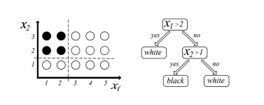
We have already used a random forrest classifier (RFC), and this method is a popular choice where deep learning has not yet made an impact. It is worthwhile to outline the concepts behind it briefly since it is also an example of a non-parametric machine learning method. The reason is that the structure of the model is defined by the training data and not conjectured at the beginning by the investigator. This fact alone helps the ease of use of this method and might explain some of its popularity, although there are additional factors that make it competitive such as the ability to build in feature selection. We will briefly outline what is behind this method. A random forest is actually an ensemble method of decision trees, so we will start by explaining what a decision tree is.
cs代写|机器学习代写machine learning代考|Linear classifiers with large margins
In this section we outline the basic idea behind support vector machines (SVM) that have been instrumental in a first wave of industrial applications due to their robustness and ease of use. A warning: SVMs have some intense mathematical underpinning, although our goal here is to outline only some of the mathematical ideas behind this method. It is not strictly necessary to read this section in order to follow the rest of the book, but it does provide a summary of concepts that have been instrumental in previous progress and are likely to influence the development of further methods and research. This includes some examples of advanced optimization techniques and the idea of kernel methods. While we mention some formulae in what follows, we do not derive all the steps and will only use them to outline the form to understand why we can apply a kernel trick. Our purpose here is mainly to provide some intuitions.
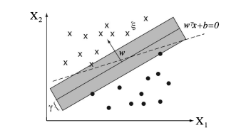
SVMs, and the underlying statistical learning theory, was largely invented by Vladimir Vapnik in the early $1960 \mathrm{~s}$, but some further breakthroughs were made in the late 1990 s with collaborators such as Corinna Cortes, Chris Burges, Alex Smola, and Bernhard Schölkopf, to name but a few. The basic SVMs are concerned with binary classification. Fig. $3.9$ shows an example of two classes, depicted by different symbols, in a 2-dimensional attribute space. We distinguish here attributes from features as follows. Attributes are the raw measurements, whereas features can be made up by combining attributes. For example, the attributes $x_{1}$ and $x_{2}$ could be combined in a feature vector $\left(x_{1}, x_{1} x_{2}, x_{2}, x_{1}^{2}, x_{2}^{2}\right)^{T}$. This will become important later. Our training set consists of $m$ data with attribute values $\mathbf{x}^{(i)}$ and labels $y^{(i)}$. We put the superscript index $i$ in brackets so it is not mistaken as a power. For this discussion we chose the binary labels of the two classes as represented with $y \in{-1,1}$. This will simplify some equations.
机器学习代写
cs代写|机器学习代写machine learning代考|Dimensionality reduction, feature selection, and t-SNE
在我们深入研究机器学习理论之前,很高兴认识到我们只触及了 sklearn 工具箱中机器学习工具的皮毛。除了分类,当然还有回归,其中标签是连续变量而不是分类变量。稍后我们将看到,我们可以将大多数有监督的机器学习技术表述为回归,而分类只是回归的一个特例。Sklearn 还包括几种聚类技术,这些技术通常是用于发现数据关系的无监督学习技术。流行的例子是 k-means 和高斯混合模型 (GMM)。我们将在后面的章节中更一般地讨论这些技术和无监督学习。在这里,我们将通过讨论一些降维方法来结束本节。
如前所述,机器学习本质上是针对高维特征空间和相应的大模型参数集的,解释机器学习结果通常并不容易。几种机器学习方法,例如神经网络或 SVM,通常被称为黑盒方法。但是,对用户没有任何隐藏;我们可以检查机器学习模型的所有部分,例如支持向量机中的权重。然而,由于模型很复杂,结果的人类可解释性具有挑战性。因此,机器学习的一个重要方面是使用互补技术,例如可视化和降维。我们已经在虹膜数据的示例中看到,即使将数据绘制在 4 维特征空间的子空间中也是有用的,我们可以询问哪个子空间最适合可视化。此外,为了帮助解决过拟合问题和计算需求,保持模型复杂度较低的一种常用技术是仔细选择输入特征。因此,这种特征选择与降维密切相关。
今天我们拥有更强大的计算机,通常更多的训练数据,以及更好的正则化技术,因此输入变量选择和独立的降维技术似乎不那么重要了。随着深度学习的出现,我们现在经常谈论从基本特征开始的端到端解决方案,而不需要预处理来找到解决方案。事实上,它可以被视为潜在信息的问题。然而,仍然有许多实际原因可以说明降维有用,例如训练数据的有限可用性和计算限制。此外,以二维地图等人类可读格式显示结果对于人机交互 (HCI) 非常有用。
仍然经常用于降维的传统方法是主成分分析(PCA)。PCA 试图找到特征表示的新坐标系,该坐标系根据数据在这些维度上的分布情况对维度进行排序。这背后的原因是,具有大量数据分布的维度将为区分数据提供最大的敏感性。如图 3.5 所示。该图中数据方差最大的方向称为第一主成分。称为第二主成分的垂直方向的方差较小。在更高的维度上,下一个主成分在更垂直的方向上,沿方向的方差减小。如果只允许使用一个量来描述数据,然后可以沿着第一个主成分选择值,因为这将捕获各个数据点之间的重要区别。当然,我们丢失了一些关于数据的信息,并且可以通过包含沿高阶主成分方向的值来更好地描述数据。用所有的主成分描述数据相当于坐标系的变换,因此相当于数据的原始描述。
cs代写|机器学习代写machine learning代考|Decision trees and random forests
正如本章开头所强调的那样,我们在这里的主要目的是表明使用 sklearn 等应用程序包可以相当容易地应用机器学习方法,尽管仍然需要知道如何使用超参数调整和平衡数据等技术才能有效使用它们。在接下来的两节中,我们将解释由随机 forrest 分类器 (RPF) 和支持向量机 (SVM) 实现的特定模型背后的一些想法。下一章将讨论神经网络。接下来的两部分是可选的,因为遵循它们背后的理论确实需要了解超出我们在本书中简要介绍性处理的其他数学概念。反而,这里的主要重点是让我们一睹这些算法背后的深刻思想,并鼓励感兴趣的读者参与进一步的研究。章节标题中的星号表示这些章节不是阅读本书其余部分的必要内容。
我们已经使用了随机 forrest 分类器 (RFC),这种方法是深度学习尚未产生影响的流行选择。值得简要概述其背后的概念,因为它也是非参数机器学习方法的一个例子。原因是模型的结构是由训练数据定义的,而不是研究者一开始就推测出来的。仅这一事实就有助于这种方法的易用性,并且可能解释了它的一些受欢迎程度,尽管还有其他因素使其具有竞争力,例如构建特征选择的能力。我们将简要概述此方法背后的内容。随机森林实际上是决策树的一种集成方法,因此我们将首先解释什么是决策树。
cs代写|机器学习代写machine learning代考|Linear classifiers with large margins
在本节中,我们将概述支持向量机 (SVM) 背后的基本思想,支持向量机因其稳健性和易用性而在第一波工业应用中发挥了重要作用。警告:SVM 有一些强大的数学基础,尽管我们在这里的目标是仅概述该方法背后的一些数学思想。为了理解本书的其余部分,阅读本节并不是绝对必要的,但它确实提供了对先前进展的重要概念的总结,并且可能会影响进一步的方法和研究的发展。这包括一些高级优化技术的例子和内核方法的想法。虽然我们在下面提到了一些公式,我们不会推导出所有的步骤,只会用它们来勾勒出表格来理解为什么我们可以应用内核技巧。我们这里的目的主要是提供一些直觉。
支持向量机和基本的统计学习理论主要是由 Vladimir Vapnik 在早期发明的1960 s,但在 1990 年代后期,与 Corinna Cortes、Chris Burges、Alex Smola 和 Bernhard Schölkopf 等合作者取得了一些进一步的突破。基本的支持向量机与二进制分类有关。如图。3.9显示了二维属性空间中由不同符号表示的两个类的示例。我们在这里将属性与特征区分开来,如下所示。属性是原始测量值,而特征可以通过组合属性来组成。例如,属性X1和X2可以组合成一个特征向量(X1,X1X2,X2,X12,X22)吨. 这将在以后变得重要。我们的训练集包括米具有属性值的数据X(一世)和标签是(一世). 我们把上标索引一世在括号中,所以它不会被误认为是一种力量。在本次讨论中,我们选择了两个类的二进制标签,如下所示是∈−1,1. 这将简化一些方程。

统计代写请认准statistics-lab™. statistics-lab™为您的留学生涯保驾护航。
金融工程代写
金融工程是使用数学技术来解决金融问题。金融工程使用计算机科学、统计学、经济学和应用数学领域的工具和知识来解决当前的金融问题,以及设计新的和创新的金融产品。
非参数统计代写
非参数统计指的是一种统计方法,其中不假设数据来自于由少数参数决定的规定模型;这种模型的例子包括正态分布模型和线性回归模型。
广义线性模型代考
广义线性模型(GLM)归属统计学领域,是一种应用灵活的线性回归模型。该模型允许因变量的偏差分布有除了正态分布之外的其它分布。
术语 广义线性模型(GLM)通常是指给定连续和/或分类预测因素的连续响应变量的常规线性回归模型。它包括多元线性回归,以及方差分析和方差分析(仅含固定效应)。
有限元方法代写
有限元方法(FEM)是一种流行的方法,用于数值解决工程和数学建模中出现的微分方程。典型的问题领域包括结构分析、传热、流体流动、质量运输和电磁势等传统领域。
有限元是一种通用的数值方法,用于解决两个或三个空间变量的偏微分方程(即一些边界值问题)。为了解决一个问题,有限元将一个大系统细分为更小、更简单的部分,称为有限元。这是通过在空间维度上的特定空间离散化来实现的,它是通过构建对象的网格来实现的:用于求解的数值域,它有有限数量的点。边界值问题的有限元方法表述最终导致一个代数方程组。该方法在域上对未知函数进行逼近。[1] 然后将模拟这些有限元的简单方程组合成一个更大的方程系统,以模拟整个问题。然后,有限元通过变化微积分使相关的误差函数最小化来逼近一个解决方案。
tatistics-lab作为专业的留学生服务机构,多年来已为美国、英国、加拿大、澳洲等留学热门地的学生提供专业的学术服务,包括但不限于Essay代写,Assignment代写,Dissertation代写,Report代写,小组作业代写,Proposal代写,Paper代写,Presentation代写,计算机作业代写,论文修改和润色,网课代做,exam代考等等。写作范围涵盖高中,本科,研究生等海外留学全阶段,辐射金融,经济学,会计学,审计学,管理学等全球99%专业科目。写作团队既有专业英语母语作者,也有海外名校硕博留学生,每位写作老师都拥有过硬的语言能力,专业的学科背景和学术写作经验。我们承诺100%原创,100%专业,100%准时,100%满意。
随机分析代写
随机微积分是数学的一个分支,对随机过程进行操作。它允许为随机过程的积分定义一个关于随机过程的一致的积分理论。这个领域是由日本数学家伊藤清在第二次世界大战期间创建并开始的。
时间序列分析代写
随机过程,是依赖于参数的一组随机变量的全体,参数通常是时间。 随机变量是随机现象的数量表现,其时间序列是一组按照时间发生先后顺序进行排列的数据点序列。通常一组时间序列的时间间隔为一恒定值(如1秒,5分钟,12小时,7天,1年),因此时间序列可以作为离散时间数据进行分析处理。研究时间序列数据的意义在于现实中,往往需要研究某个事物其随时间发展变化的规律。这就需要通过研究该事物过去发展的历史记录,以得到其自身发展的规律。
回归分析代写
多元回归分析渐进(Multiple Regression Analysis Asymptotics)属于计量经济学领域,主要是一种数学上的统计分析方法,可以分析复杂情况下各影响因素的数学关系,在自然科学、社会和经济学等多个领域内应用广泛。
MATLAB代写
MATLAB 是一种用于技术计算的高性能语言。它将计算、可视化和编程集成在一个易于使用的环境中,其中问题和解决方案以熟悉的数学符号表示。典型用途包括:数学和计算算法开发建模、仿真和原型制作数据分析、探索和可视化科学和工程图形应用程序开发,包括图形用户界面构建MATLAB 是一个交互式系统,其基本数据元素是一个不需要维度的数组。这使您可以解决许多技术计算问题,尤其是那些具有矩阵和向量公式的问题,而只需用 C 或 Fortran 等标量非交互式语言编写程序所需的时间的一小部分。MATLAB 名称代表矩阵实验室。MATLAB 最初的编写目的是提供对由 LINPACK 和 EISPACK 项目开发的矩阵软件的轻松访问,这两个项目共同代表了矩阵计算软件的最新技术。MATLAB 经过多年的发展,得到了许多用户的投入。在大学环境中,它是数学、工程和科学入门和高级课程的标准教学工具。在工业领域,MATLAB 是高效研究、开发和分析的首选工具。MATLAB 具有一系列称为工具箱的特定于应用程序的解决方案。对于大多数 MATLAB 用户来说非常重要,工具箱允许您学习和应用专业技术。工具箱是 MATLAB 函数(M 文件)的综合集合,可扩展 MATLAB 环境以解决特定类别的问题。可用工具箱的领域包括信号处理、控制系统、神经网络、模糊逻辑、小波、仿真等。